1. INTRODUCTION
Inertial Navigation Systems (INS) are widely applied in land, marine and aircraft navigation owing to their characteristics of complete independency from outside navigation transmissions, potential for stealthy operation and relative independence from the environment they are operated in (Titterton and Weston, Reference Titterton and Weston2004). An INS generates Shuler, Foucault and Earth periodic oscillation errors motivated by error sources when it works in an undamped mode. For long-term INS, oscillation errors greatly affect the precision of navigation, so it is essential to suppress them. Damping technology is an effective way to suppress INS oscillation errors. By introducing damping, an INS can be transformed from a critical but stable system to a stable system. Thus, the goal of suppressing oscillation errors is achieved. A Kalman filter can also be used to compensate the oscillation errors (Zhao et al., Reference Zhao, Li, Cheng and Hao2016). After introducing damping, the original Shuler tuning condition of the INS is destroyed. When a vehicle carrying an INS operates in a manoeuvring condition, damping will have a negative influence on the output of the INS. Thus, damping technology can only be used in the non-manoeuvring condition. To counter this problem, it is common to switch modes according to the carrier's operating state. In other words, if the carrier operates in a manoeuvring condition, the INS is switched to an undamped mode. If the carrier operates in a non-manoeuvring condition, the INS is switched to a damped mode. However, overshoot is an inevitable phenomenon in the process of switching and needs to be decreased as much as possible to ensure accuracy.
In order to improve this situation, two main categories of methods are used (Jiang et al., Reference Jiang, Yu and Chen2014; He et al., Reference He, Xu and Qin2012; Cheng et al., Reference Cheng, Zhao and Song2005a; Qin et al., Reference Qin, Li and Xu2011). The first method is mainly based on qualitative analysis, and the overshoot generated by switching is related to the closed-loop damping ratio of the system. By gradually increasing the damping ratio of the system from zero to a steady state value, the overshoot process can be reduced. However, increasing the damping ratio of the system will also slow down the convergence rate of oscillation error, which is not good for the system. Changing the damping ratio essentially means switching between systems with different damping ratios. If the damping ratio is not properly selected, the accuracy of the INS is reduced. The second method is based on the command rate before and after the switching. Through introduction of compensation, the command rate will not change before and after the switching, thereby weakening the overshoot. However, the second method needs accurate position and related information provided by external devices such as Global Navigation Satellite Systems (GNSS) and this can limit its application fields.
These methods compensate errors but do not focus on the cause of the problem. Switching is the essence of this problem. Therefore, this paper aims at solving the problem from the perspective of a switched system without external information. The switching process plays a decisive role in the stability of the system. In order to apply the switching system to the actual project, stability analysis is an indispensable step.
A switched system is a typical hybrid system which consists of several subsystems and a switching law coordinating the operation of each subsystem. Many control theories and methods have been established in the switching field (Hu et al., Reference Hu, Zhai and Michael2000). Many researchers have investigated switched systems, which have broad application in real life systems such as for robot control (Tan et al., Reference Tan, Xi and Wang2004), electrical power systems (Williams and Hoft, Reference Williams and Hoft1991) and spacecraft control (Oishi and Tomlin, Reference Oishi and Tomlin1999). Switched systems can achieve good performance by switching control regimes. INS also have a problem of switching between two operating modes, but published work into similar research from the perspective of switched systems is difficult to find.
In this paper, the damped and undamped modes of an INS as a switched system controlled by a switching controller is investigated, with the first aspect considered being stability. The stability of a switched system is divided into three basic problems (Liberzon and Morse, Reference Liberzon and Morse1999). Lyapunov functions (Branicky, Reference Branicky1994; Dayawansa and Martin, Reference Dayawansa and Martin1999; Mancilla-Aguilar, Reference Mancilla-Aguilar2000; Mason and Shorten, Reference Mason and Shorten2007; King and Shorten, Reference King and Shorten2004; Cheng, Reference Cheng2004) and dwell time method (Lee et al., Reference Lee, Kim and Lim2000; Zhai et al., Reference Zhai, Hu, Yasuda and Michel2001; Mancilla-Aguilar and Garcia, Reference Mancilla-Aguilar and Garcia2006; Hespanha et al., Reference Hespanha, Liberzon, Angeli and Sontag2005) are the main methods used to solve the stability of the system. For stability under arbitrary switching signals, the main research method is the single Lyapunov function method. The idea of the single Lyapunov function method is that if all subsystems exist within a common Lyapunov function, then the switched system is stable under an arbitrary switching signal. In practical applications, the switching signal is often constrained. The multi-Lyapunov function method and the dwell time method are common ways to deal with the system under a constraint switching signal. The idea of the multiple Lyapunov function method is that if there exist different Lyapunov functions for different subsystems, the corresponding Lyapunov function value will become smaller when each subsystem is working properly and then the switching system is stable under the constrained switching signal. The idea of the dwell time method is that if the dwell time on a stable subsystem is long enough so that the energy decay of the stable subsystem can completely offset and exceed the energy increase caused by the switching, then the switching system is stable under a constrained switching signal. The average dwell time method proposed by Hespanha (Reference Hespanha1999) is based on the dwell time method. The main idea here is that allowing the action time of some of the subsystems to be less than a certain dwell time, but ensuring the average dwell time of all subsystems is not less than this certain dwell time, then the switched system under constrained switching signals is stable. An INS works in damping mode most of the time. When it is necessary, it is switched to the undamped mode. The average dwell time method is used here to analyse the stability.
In this paper, a switched control is introduced into the damped and undamped INS switching problem. A model of a switching problem is established, and sufficient conditions for system stability are obtained. Under the condition of stability, the overshoot causes are analysed, and switched control is introduced to verify the effectiveness of the controller.
This paper is organised as follows: the model of INS operating in damped and undamped modes is established in Section 2. Section 3 analyses stability and gives the sufficient condition of exponential stability. The switching compensation controller is designed for a long-term INS in Section 4 and Section 5 verifies the effectiveness of the switched control. Section 6 gives the conclusions.
2. FORMULATION
Generally, the model of a switched system is described as:
 $$\dot{x}=f_\sigma \lpar x\lpar t\rpar \comma \; u\lpar t\rpar \comma \; w\lpar t\rpar \rpar $$
where x(t) ∈ ℝn is the system state, u(t) ∈ ℝm is the control input, w(t) is the disturbance,  $\dot {x}=f_{i} \lpar x\lpar t\rpar \comma \; u\lpar t\rpar \comma \; w\lpar t\rpar \rpar $ is the i-th subsystem,
  $i\in {\cal I}=\lcub 1\comma \; 2\comma \; \ldots \comma \; N\rcub $, N is the total number of subsystems and the switching law
  $\sigma \colon \lsqb t_{0} \comma \; \infty \rpar \to {\cal I}$ is a right continuous segmentation constant function. A typical switched system diagram is shown in Figure 1.
Figure 1. A typical switched system diagram.
For INS, the switched system has two operating modes, the damped inertial navigation mode and the undamped inertial navigation mode corresponding to two different subsystems. We take the north loop as an example to derive the INS model.
A north loop error block diagram of an undamped INS is shown in Figure 2. In Figure 2, ∇E is the bias of east accelerometer, ϕ N is the north misalignment angle, ε N is the north gyro drift, δ V E is the east velocity error, g is the gravitational acceleration and R is Earth's radius.
Figure 2. North loop error block diagram of an undamped INS.
From Figure 2, we can obtain the relationship of ϕ N and ε N:
 $$\displaystyle{{{\phi}_N\lpar s\rpar } \over {\varepsilon _N\lpar s\rpar }} = \displaystyle{s \over {s^2 + \displaystyle{g \over R}}} $$
Equation (2) indicates that the roots of the north loop characteristic equation of an undamped system is a pair of conjugate complex roots. Therefore, the north loop is a critical but stable system. In order to eliminate oscillation, the horizontal damping network H(s) is added to the damped north loop.
A north loop error block diagram with a horizontal damping system is shown in Figure 3.

Figure 3. North loop error block diagram of horizontal damping system.
After adding H(s), the characteristic equation of the north loop becomes:
 $$s^2 + \displaystyle{g \over R}H\lpar s\rpar = 0 $$
If H(s) is designed properly, the north loop will be damped so that the oscillation is eliminated.
In order to solve the switching problem, the idea of using a switched system is proposed. These two subsystems must be described in a unified form to construct the switched system.
In the north loop error block diagram of the undamped INS, H(s) is equal to 1. These two block diagrams can be combined, and this is shown in Figure 4.

Figure 4. Error block diagram of north loop switching controller where u is the output of the controller.
Using Figure 4, we can obtain the model of the switched system:
 $$\left\{\matrix{{\delta \dot {V}_E =-{\phi}_N g+\nabla_E } \hfill \cr {\dot {\phi}_N =\displaystyle{1 \over R}u+\varepsilon_N } \hfill \cr}\right. $$
Changing it to matrix form:
 $$\left[\matrix{{\delta \dot {V}_E} \cr {\dot {\phi}_N } \cr }\right]=\left[\matrix{0 & {-g} \cr 0 & 0 \cr } \right]\left[\matrix{{\delta V_E } \cr {{\phi}_N } \cr } \right]+ \left[\matrix{0 \cr {\displaystyle{1 \over R}} \cr } \right]u+\left[\matrix{{\nabla_E } \cr {\varepsilon_N } \cr } \right]$$
 $$u=K\left[\matrix{{\delta V_E } \cr {{\phi}_N} \cr } \right]$$
where K is the controller.
Therefore, we can establish the state space error model of INS:
 $$\eqalign{{\dot x} & =Ax+Bu+w \cr y & =Cx} $$
where  $A=\left[\matrix{0 & {-g} \cr 0 & 0 \cr } \right]$,
  $B=\left[\matrix{0 \cr {\displaystyle{{1}\over{R}}} \cr } \right]$,
  $C=\left[\matrix{0 & 1 \cr } \right]$,
  $x=\left[\matrix{{\delta V_{E} } \cr {{\phi}_{N} } \cr } \right]$,
  $u=K\left[\matrix{{\delta V_{E} } \cr {{\phi}_{N} } \cr } \right]$,
  $w=\left[\matrix{{\nabla_{E} } \cr {\varepsilon_{N} } \cr } \right]$.
In order to analyse the controllability of the system, the controllability matrix Q c is calculated:
 $$Q_c =\left[\matrix{B & {AB} \cr } \right]=\left[\matrix{0 & {-\displaystyle{g \over R}} \cr {\displaystyle{1 \over R}} & 0 \cr } \right]$$
From Equation (8), we can see that rankQ c = 2 and the controllability matrix of the system is full rank. Therefore, the system is completely controllable. The expression u is the form of state feedback. Therefore, if we consider the damped and undamped problem of an INS with respect to control, it can be described as: The operating state of the INS is determined by the switching controller. The switching controller determines the operating mode of the whole system and directly determines the performance of the system, that is, the accuracy of the system.
Substituting u into Equation (7), we have:
 $$\dot {x}=\lpar A+BK\rpar x+w $$
For an undamped INS, the eigenvalue of matrix A + BK is a pair of conjugate imaginary roots, which makes the system critical but stable. While for a damped INS, the real part of the eigenvalue of matrix A + BK can be made negative by designing K properly which makes the system stable.
The model of the switched system of the problem is described as follows.
Consider the switched system:
 $$\dot {x}\lpar t\rpar = A_{\sigma \lpar t\rpar } \lpar t\rpar x\lpar t\rpar +B_{\sigma \lpar t\rpar } \lpar t\rpar u\lpar t\rpar +Dw\comma \; x\lpar t_0 \rpar =x_0 $$
 $$y = C_{\sigma \lpar t\rpar } \lpar t\rpar x\lpar t\rpar $$
where x(t) ∈ ℝn is the system state, t 0 is the initial time, x 0 is the initial state, u(t) ∈ Ω ⊂ ℝm is the control input constrained to the convex and compact set Ω, y(t) ∈ ℝq is the output, w ∈ ℝp is the constant disturbance and D ∈ ℝn×p, σ(t) : [t 0, ∞) → {1, 2, …, N} is a piecewise constant function called the switching law. Thus A σ(t)(t) ∈ ℝn×n, B σ(t)(t) ∈ ℝn×m and C σ(t)(t) ∈ ℝq×n are piecewise functions since A σ(t)(t) : [t 0, ∞) → {A 1(t), A 2(t), …, A N(t)}, B σ(t)(t) : [t 0, ∞) → {B 1(t), B 2(t), …, B N(t)} and C σ(t)(t) : [t 0, ∞) → {C 1(t), C 2(t), …, C N(t)}. Here, {A 1(t), A 2(t), …, A N(t)}, {B i(t), B 2(t), …, B N(t)} and {C 1(t), C 2(t), …, C N(t)} are matrices describing the subsystems.
A function u(t) = K σ(t) x(t) is called the state feedback law. K σ (t) is a set of feedback gain matrices {K 1(t), K 2(t), …, K N(t)} such that the switched linear system becomes a closed loop system:
 $$\dot {x}\lpar t\rpar =\lpar A_{\sigma \lpar t\rpar } \lpar t\rpar +B_{\sigma \lpar t\rpar } \lpar t\rpar K_{\sigma \lpar t\rpar } \lpar t\rpar \rpar x\lpar t\rpar +Dw $$
In switched system Equation (10), we make Assumption 1:
Assumption 1: Let N = 2, A 1(t) + B 1(t) K 1(t) is a system that is unstable from state feedback and A 2(t) + B 2(t) K 2(t) is a system that is stable from state feedback.
If Assumption 1 is satisfied, system Equation (10) is the model of the damped and undamped INS problem.
Since the entire system needs to be switched between the two modes, the stability of the system Equation (10) is now analysed in order to ensure stability during the switching process.
3. STABILITY ANALYSIS OF AN INERTIAL NAVIGATION SWITCHED SYSTEM
In this section, we analysed the stability of switched system Equation (10). First, we give the definition of exponential stability. The switched system Equation (10) is said to be exponentially stable if there exists a positive number c and a positive number λ such that the equation:
 $$\Vert x\lpar t\rpar \Vert \le ce^{-\lambda \lpar t-t_0 \rpar } \Vert x\lpar 0\rpar \Vert \comma \; \quad t\ge t_0 $$
holds.
For ease of analysis, we first analyse the stability of the system without disturbance.
3.1. Stability analysis without disturbance
The system without disturbance can be described as:
 $$\dot {x}\lpar t\rpar =A_{\sigma \lpar t\rpar } \lpar t\rpar x\lpar t\rpar +B_{\sigma \lpar t\rpar } \lpar t\rpar u\lpar t\rpar \comma \; x\lpar t_0 \rpar =x_0 $$
where the symbols have the same meaning as system Equation (10).
In order to analyse the stability of the system, the concept of average dwell time, proposed by Hespanha (Reference Hespanha1999) is introduced. For each switching law σ (t) and each t > τ ≥ t 0, let N σ(τ, t) denote the number of switchings of σ over the interval (τ, t). For given N 0, τ a > 0, let S a[τ a, N 0] denote the set of all switching signals satisfying:
 $$N_\sigma \lpar \tau \comma \; t\rpar \le N_0 + \displaystyle{{t-\tau } \over {\tau _a}} $$
where the constant τ a is called the average dwell time and N 0 denotes the chatter bound.
Denote b 1 as the number of activated unstable subsystems over [t 0, t], and denote b 2 as the number of activated stable subsystems over [t 0, t]. Thus:
 $$b_1 +b_2 =N_\sigma \lpar t_0 \comma \; t\rpar $$
For any switching signal σ (t), denote T + (t 0, t) as the total activation time of uncontrollable subsystems on [t 0, t), and denote T − (t 0, t) as the total activation time of controllable subsystems on [t 0, t). It can be seen that:
 $$T_+ \lpar t_0 \comma \; t\rpar +T_- \lpar t_0 \comma \; t\rpar =t-t_0 $$
The condition:
 $$\displaystyle{{T_-\lpar t_0\comma \; t\rpar } \over {T_ + \lpar t_0\comma \; t\rpar }} \gt \beta $$
holds for some β > 0 and arbitrary t > t 0 ≥ 0. From Equations (17) and (18), we have:
 $$T_ + \lpar t_0\comma \; t\rpar \le \displaystyle{1 \over {1 + \beta }}\lpar t-t_0\rpar \comma \; T_-\lpar t_0\comma \; t\rpar \ge \displaystyle{\beta \over {1 + \beta }}\lpar t-t_0\rpar $$
In order not to lose generality, we make the following assumptions:
Assumption 2:
(1) Assume that after introducing state feedback, (A 1, B 1, K 1), …, (A p, B p, K p) are unstable and (A p+1, B p+1, K p+1), …, (A N, B N, K N) are stable.
(2) Average dwell time is no less than τ a.
Define:
 $$\lambda _+ =\mathop {\max }\limits_{1\le i \lt p} \lambda_p $$
To prove the stabilisation of the closed loop system, we make use of the following lemma.
Lemma 1 (Cheng et al., Reference Cheng, Guo and Wang2005b):
Let A ∈ ℝn×n and B ∈ ℝn×m be two matrices such that the pair (A, B) is controllable. Let τ > 0, then for δ > 0, there exists a positive number λ and a matrix K ∈ ℝm×n such that:
 $$\Vert e^{\lpar A+BK\rpar t}\Vert \le \delta e^{-\lambda \lpar t-\tau \rpar }\comma \; t\ge 0 $$
Lemma 1 shows that through the state feedback, we can arbitrarily configure the poles of the system so that they are located at the left half of the s plane. This is applicable for (A p+1, B p+1, K p+1), …, (A N, B N, K N) that are stable subsystems after introducing state feedback. However, for (A 1, B 1, K 1), …(A p, B p, K p), this is not applicable. For the latter, we need to consider it separately. From Lemma 1, Lemma 2 can be obtained:
Lemma 2:
Let A ∈ ℝn×n and B ∈ ℝn×m be two matrices such that the pair (A, B) is controllable. If matrix K ∈ ℝm×n makes matrix A + BK have non-negative eigenvalues, let τ > 0 and there exists c > 0 and λ > 0 such that:
 $$\Vert e^{\lpar A+BK\rpar t}\Vert \le ce^{\lambda \lpar t-\tau \rpar }\comma \; t\ge 0 $$
 Proof. A is a n dimension matrix, n distinct numbers λ 1, λ 2, …, λ n are chosen, where the number of the conjugate virtual root is m.  $\alpha \lpar s\comma \; \lambda \rpar =\Pi _{i=1}^{n} \lpar s+\lambda _{i} \rpar $ is a monic polynomial of degree n in s. Since (A, B) is controllable, there exists a polynomial matrix H(λ) corresponding with A + BK which makes the characteristic polynomial α(s, λ).
Therefore, there exists a matrix T such that matrix A + BK is diagonalisable (T −1(A + BK) T = Λ = diagonal). T −1 has the same character. Let λ = max{λ 1, λ 2, …, λ n}, according to e (A+BK) t = T −1e Λ tT and  $\vert e^{\Lambda t}\vert \le \lpar \sqrt 2 \rpar ^{m}ne^{\lambda t}$, we have:
 $$\vert e^{\Lambda t}\vert \le \rho e^{\lambda t}\comma \; t\ge 0 $$
where  $\rho =\lpar \sqrt 2 \rpar ^{m}n\vert T^{-1}\vert \vert T\vert $.
Remark: Lemma 1 uses state feedback to attenuate the controllable at the rate of e −λ t and Equation (21) holds. Lemma 2 estimates the condition that the controllable system still has non-negative eigenvalues by state feedback.
Theorem 1:
Let Assumptions 1 and 2 hold for the closed loop system Equation (12), and there exists a set of feedback gain matrices {K 1(t), K 2(t), …, K N(t)} which makes the system Equation (12) exponentially stable under state feedback and the switching law.
Proof. Set:
 $$L=\max \lcub c\comma \; \delta \rcub $$
 For any  $\tau _{a}^{\ast} \gt0$ and β > 0, choose λ sufficiently large such that:
 $$c_1 = \displaystyle{{\lambda \beta -\lambda _ + } \over {1 + \beta }}-\displaystyle{{\ln L} \over {\tau _a^{\ast}}} \gt 0 $$
For t ≥ t 0, assume that t k ≤ t < t k+1 and σ(t) = i k. If i k ∈ {p + 1, p + 2, …, N}, we have:
 $$\eqalign{\Vert x\lpar t\rpar \Vert & \le \delta e^{-\lambda \lpar t-t_k \rpar } \Vert x\lpar t_k \rpar \Vert \cr & \le Le^{-\lambda \lpar t-t_k\rpar } \Vert x\lpar t_k \rpar \Vert } $$
If i k ∈ {1, 2, …, p}, we have:
 $$\eqalign{\Vert x\lpar t\rpar \Vert & \le ce^{\lambda \lpar t-t_k \rpar }\Vert x\lpar t_k \rpar \Vert \cr & \le Le^{\lambda \lpar t-t_k \rpar }\Vert x\lpar t_k \rpar \Vert} $$
 Similarly, there exist a series of feedback matrices  $\lcub K_{i_{j-1} } \rcub $ for j ∈ {1, 2, …k} such that:
 $$\Vert x\lpar t_j \rpar \Vert \le \left\{\matrix{{Le^{-\lambda \lpar t-t_k \rpar }\Vert x\lpar t_k \rpar \Vert \comma \; \sigma \lpar t_{j-1} \rpar \in \lcub p+1\comma \; \ldots \comma \; N\rcub } \hfill \cr {Le^{\lambda \lpar t-t_k \rpar }\Vert x\lpar t_k \rpar \Vert \comma \; \sigma \lpar t_{j-1} \rpar \in \lcub 1\comma \; 2\comma \; \ldots \comma \; p\rcub }\hfill \cr}\right. $$
 Therefore, under the feedback law  $u\lpar t\rpar =K_{i_{j} } x\lpar t\rpar $for j ∈ {1, 2, …k}, from Equations (26)–(28) we obtain Equation (29) by induction:
 $$\eqalign{\Vert x\lpar t\rpar \Vert & \le L^{j_2 }e^{-\lambda T_- \lpar t_0 \comma t\rpar }L^{j_1 }e^{\lambda _+ T_+ \lpar t_0 \comma t\rpar }\Vert x_0 \Vert \cr & \le L^{j_1 +j_2 }e^{-\lambda T_- \lpar t_0 \comma t\rpar +\lambda _+ T_+ \lpar t_0 \comma t\rpar }\Vert x_0 \Vert \cr & =e^{N_\sigma \lpar t_0 \comma t\rpar \ln L+\lambda _+ T_+ \lpar t_0 \comma t\rpar -\lambda T_- \lpar t_0 \comma t\rpar }\Vert x_0 \Vert} $$
Noting that:
 $$N_\sigma \lpar t_0\comma \; t\rpar \le \displaystyle{{t-t_0} \over {\tau _a^{\ast} }} $$
From Equations (18), (20), (28) and (29), we get:
 $$\eqalign{\Vert x\lpar t\rpar \Vert & \le e^{\displaystyle{{\ln L} \over {\tau _a^* }}\lpar t-t_0\rpar + \displaystyle{{\lambda _ + } \over {1 + \beta }}\lpar t-t_0\rpar -\displaystyle{{\lambda \beta } \over {1 + \beta }}\lpar t-t_0\rpar }{\rm \Vert }x_0{\rm \Vert } \cr & = e^{-\lpar \displaystyle{{\lambda \beta -\lambda _ + } \over {1 + \beta }}-\displaystyle{{\ln L} \over {\tau _a^* }}\rpar \lpar t-t_0\rpar }{\rm \Vert }x_0{\rm \Vert } \cr &=e^{-c_1 \lpar t-t_0 \rpar }\Vert x_0 \Vert} $$
where c 1 > 0 is defined by Equation (25).
Remark: System Equation (10), can be stabilised by the average dwell time method, which provides theoretical principles for further study of system switching.
3.2. Stability analysis with disturbance
In this section, we consider the stability of the system with disturbance.
The plant is described as:
 $$\dot {x}\lpar t\rpar =A_{\sigma \lpar t\rpar } \lpar t\rpar x\lpar t\rpar +B_{\sigma \lpar t\rpar } \lpar t\rpar u\lpar t\rpar +Dw\comma \; x\lpar t_0 \rpar =x_0 $$
where the symbols have the same meaning as in system Equation (10).
In this section, we make the following assumption:
Assumption 3: There exists μ such that:
 $$\Vert Dw\Vert \le \mu \Vert x\Vert $$
where μ ≥ 0.
The stability of a system with disturbance is calculated by solving the differential equation directly.
For an arbitrary t > 0, let t 0 < t 1 < · · · < t i ≤ t < t i+1, where t j(j = 1, 2, …, i) is the switching time. Assuming that in [t j−1, t j), the p j th subsystem is active. Solving the differential Equation (32), we have:
 $$\eqalign{& x\lpar t_1 \rpar =e^{\lpar A_1 +B_1 K_1 \rpar \lpar t_1 -t_0 \rpar }x\lpar t_0 \rpar +\vint_{t_0 }^{t_1 } {e^{\lpar A_1+B_1 K_1 \rpar \lpar t_1 -s\rpar }} f_1 \lpar x\lpar s\rpar \rpar ds \cr & x\lpar t_2 \rpar =e^{\lpar A_2 +B_2 K_2 \rpar \lpar t_2 -t_1 \rpar }x\lpar t_1 \rpar +\vint_{t_1 }^{t_2 } {e^{\lpar A_2+B_2 K_2 \rpar \lpar t_2 -s\rpar }} f_2 \lpar x\lpar s\rpar \rpar ds \cr & \cdots \cr & x\lpar t\rpar =e^{\lpar A_{i+1} +B_{i+1} K_{i+1} \rpar \lpar t-t_i \rpar }x\lpar t_i \rpar +\vint_{t_i }^t {e^{\lpar A_{i+1} +B_{i+1} K_{i+1} \rpar \lpar t-s\rpar }} f_{i+1} \lpar x\lpar s\rpar \rpar ds} $$
According to (34), we have:
 $$\eqalign{x\lpar t\rpar & =e^{\lpar A_{i+1} +B_{i+1} K_{i+1} \rpar \lpar t-t_i \rpar }\cdots e^{\lpar A_2 +B_2 K_2 \rpar \lpar t_2-t_1 \rpar }x\lpar t_1 \rpar e^{\lpar A_1 +B_1 K_1 \rpar \lpar t_1 -t_0 \rpar }x\lpar t_0 \rpar x\lpar t_0 \rpar \cr & \quad +\vint_{t_0 }^{t_1 } {e^{\lpar A_{i+1} +B_{i+1} K_{i+1} \rpar \lpar t-t_i \rpar }} \cdots e^{\lpar A_2 +B_2 K_2 \rpar \lpar t_2 -t_1 \rpar }e^{\lpar A_1 +B_1 K_1 \rpar \lpar t_1 -s\rpar }f_1 \lpar x\lpar s\rpar \rpar ds \cr & \quad +\vint_{t_1 }^{t_2 } {e^{\lpar A_{i+1} +B_{i+1} K_{i+1} \rpar \lpar t-t_i \rpar }} \cdots e^{\lpar A_2 +B_2 K_2 \rpar \lpar t_2 -s\rpar }f_2 \lpar x\lpar s\rpar \rpar ds \cr & \quad +\cdots \cr & \quad +\vint_{t_{i-1} }^{t_i } {e^{\lpar A_{i+1} +B_{i+1} K_{i+1} \rpar \lpar t-t_i \rpar }}e^{\lpar A_i +B_i K_i \rpar \lpar t_i -s\rpar }f_i \lpar x\lpar s\rpar \rpar ds \cr & \quad +\vint_{t_i }^t {e^{\lpar A_{i+1} +B_{i+1} K_{i+1} \rpar \lpar t_i -s\rpar }} f_{i+1}\lpar x\lpar s\rpar \rpar ds} $$
 The first item on the right side of Equation (35),  $e^{\lpar A_{i+1} +B_{i+1} K_{i+1} \rpar \lpar t-t_{i} \rpar }\cdots e^{\lpar A_{2} +B_{2} K_{2} \rpar \lpar t_{2} -t_{1} \rpar } e^{\lpar A_{1} +B_{1} K_{1} \rpar \lpar t_{1} -t_{0} \rpar }x\lpar t_{0} \rpar $ corresponds to the non-disturbed switching system in [t 0, t), while the item
  $e^{\lpar A_{i+1} +B_{i+1} K_{i+1} \rpar \lpar t-t_{i} \rpar }\cdots e^{\lpar A_{j} +B_{j} K_{j} \rpar \lpar t-s\rpar }$ corresponds to the switching system in [s, t). Equation (36) can be obtained:
 $$\eqalign{& \Vert e^{\lpar A_{i+1} +B_{i+1} K_{i+1} \rpar \lpar t-t_i \rpar }\cdots e^{\lpar A_2 +B_2 K_2 \rpar \lpar t_2 -t_1\rpar }e^{\lpar A_1 +B_1 K_1 \rpar \lpar t_1 -t_0 \rpar }x\lpar t_0 \rpar x\lpar t_0 \rpar \Vert \cr & \le e^{-c_1 \lpar t-t_0 \rpar }\Vert e^{\lpar A_{i+1} +B_{i+1} K_{i+1} \rpar \lpar t-t_i \rpar }\cdots e^{\lpar A_j+B_j K_j \rpar \lpar t-s\rpar }\Vert \cr & \le e^{-c_1 \lpar t-s\rpar }} $$
where c 1 is defined as in Equation (25). According to Equations (33) and (36), we have:
 $$\Vert x\lpar t\rpar \Vert \le e^{-c_1 \lpar t-t_0 \rpar }\Vert x_0 \Vert +\vint_{t_0 }^t {e^{-c_1 \lpar t-s\rpar }} \lpar \mu \Vert x\Vert \rpar ds $$
Therefore:
 $$\Vert x\lpar t\rpar \Vert e^{c_1 t}\le e^{c_1 t_0 }\Vert x_0 \Vert +\vint_{t_0 }^t \mu e^{-c_1 s}\Vert x\Vert ds $$
In order to prove the stability, we need the following lemma.
Lemma 3 (Dragomir, Reference Dragomir2003):
Let y(t) and h(t) be real continuous function defined on [a, b] with b > a > 0, h(t) ≥ 0 for t ∈ [a, b], c ≥ 0 is a constant. Then:
 $$y\lpar t\rpar \le c+\vint_a^t h \lpar s\rpar y\lpar s\rpar ds\comma \; t\in \lsqb a\comma \; b\rsqb $$
implies that:
 $$y\lpar t\rpar \le ce^{\vint_a^t h \lpar s\rpar ds}\comma \; t\in \lsqb a\comma \; b\rsqb $$
Theorem 2:
Let Assumptions 1–3 hold, if there exists a positive number μ such that c 1 > μ, where:
 $$c_1 = \displaystyle{{\lambda _\beta -\lambda _ + } \over {1 + \beta }}-\displaystyle{{\ln L} \over {\tau _a^* }} > 0$$
then the system Equation (32) is stable.
Proof. According to Equation (38) and Lemma 3, the following can be obtained:
 $$\eqalign{\Vert x\lpar t\rpar \Vert e^{c_1 t} & \le e^{c_1 t_0 }\Vert x_0 \Vert +\vint_{t_0 }^t \mu e^{-c_1 s}\Vert x\Vert ds \cr &\le e^{c_1 t_0 }e^{\vint_{t_0 }^t \mu ds}\Vert x_0 \Vert \cr &=e^{c_1 t_0 }e^{\mu \lpar t-t_0 \rpar }\Vert x_0 \Vert} $$
 Multiply both sides of the equation with  $e^{-c_{1} t}$:
 $$\eqalign{\Vert x\lpar t\rpar \Vert & \le e^{-c_1 t}e^{c_1 t_0 }e^{\mu \lpar t-t_0 \rpar }\Vert x_0 \Vert \cr &=e^{-\lpar c_1 -\mu \rpar \lpar t-t_0 \rpar }\Vert x_0 \Vert} $$
Thus, when c 1 − μ> 0, that is c 1 > μ, the system is exponentially stable.
4. SWITCHING COMPENSATION CONTROL OF LONG-TERM INERTIAL NAVIGATION
Under the condition of system stability, the overshooting error caused by switching is only determined by the calculation of the speed at the switching moment (Feng, Reference Feng2016):
 $$\phi _N\lpar s\rpar = \displaystyle{{H_x\lpar s\rpar -1} \over {rs^2 + gH_x\lpar s\rpar }}v_{E1}^c $$
where ϕ N(s) is the north misalignment angle, H x (s) is the horizontal damping network and  $v_{E1}^{c} $ is the calculated eastward speed.
When switching happens, in order to reduce the overshoot caused by switching, the switching compensation controller is added at different speeds to reduce overshoot at the corresponding speed by switched control. The switching compensation controller consists of three parts: dead-zone, differential part and proportional part. The dead zone part controls the start moment. The differential part and the proportional part control the overshoot magnitude. After adding a switching compensation controller, the system diagram is shown in Figure 5.

Figure 5. Error block diagram of north loop of switching controller with switching compensation controller.
In Figure 5,  $k\displaystyle{{du} \over {dt}}$ is the differential part and proportional part, the second part is the dead-zone.
Remark: The switching compensation controller is available only when switching happens. When the system operates steadily, the controller makes no difference to the system.
5. EXPERIMENT
5.1. Verification of switching stability
Consider the actual damped and undamped INS, where:
 $$\eqalign{A_1 &=\left[\matrix{0 & {-9.8} \cr 0 & 0 \cr } \right]\comma \; B_1 =\left[\matrix{0 \cr {\displaystyle{1 \over R}} \cr } \right]\cr A_2 &=\left[\matrix{0 & {-9.8} \cr 0 & 0 \cr } \right]\comma \; B_2 =\left[\matrix{0 \cr {\displaystyle{1 \over R}} \cr } \right]\cr D & =\left[\matrix{1 & 0 \cr 0 & 1 \cr } \right]\comma \; w=\left[\matrix{{10^{-5}} \cr {0.01} \cr } \right]}$$
 According to the practical model of damping and undamped system, the switching controller  $K_{1} =\left[\matrix{{-1} & 0 \cr } \right]\comma \; K_{2} =\left[\matrix{{-52.17} & {114806.47} \cr } \right]$ can be obtained. Under the state feedback u(t) = K σ x(t), the closed loop system is obtained. Then:
 $$\Vert Dw\Vert _\infty =0.01$$
In an INS, states of the system are bounded, then:
 $$\Vert x\Vert \le M$$
where M is the supremum of the system. If ‖x‖ ≤ 1, let ‖x‖ = 1 in case ‖x‖ is too small which will influence the choice of other parameters.
Choosing  $\mu = \max \lcub \displaystyle{{2 \times 0.01} \over {{\Vert}x{\Vert}}}\comma \; 1\rcub $, then Assumption 2 holds.
Let c = δ= 30, then L = 30. According to A 1, A 2, λ + = 0 can be obtained. Let τ a* = 2, β = 1 and λ = 6, then:
 $$c_1 = \displaystyle{{\lambda _\beta -\lambda _ + } \over {1 + \beta }}-\displaystyle{{\ln L} \over {\tau _a^* }} = \displaystyle{{6-0} \over {1 + 1}}-\displaystyle{{\ln 30} \over 2} = 1.30 > \mu = 1$$
By Theorem 2, the switched system is exponentially stable.
5.2. Switched control simulation experiment
The simulation time was 10 hours. The carrier sailed at a constant velocity of  $\lsqb \matrix{{5m/s} & 0 & 0 }\rsqb ^{T}\comma \; \lsqb \matrix{{10m/s} & 0 & 0 }\rsqb ^{T}$ and
  $\lsqb \matrix{{15m/s} & 0 & 0 }\rsqb ^{T}$respectively. The initial attitude was
  $\lsqb \matrix{0 & 0 & 0}\rsqb ^{T}$. The initial position was
  $\lsqb \matrix{{30^{\circ} } & {120^{\circ} } & 0}\rsqb ^{T}$. Sensor parameters are shown in Table 1. The initial north misalignment angle was 1 '. At 2 h, the inertial navigation system enters the damping mode.
Table 1. Sensor Parameters
The experimental results are shown in Figure 6.
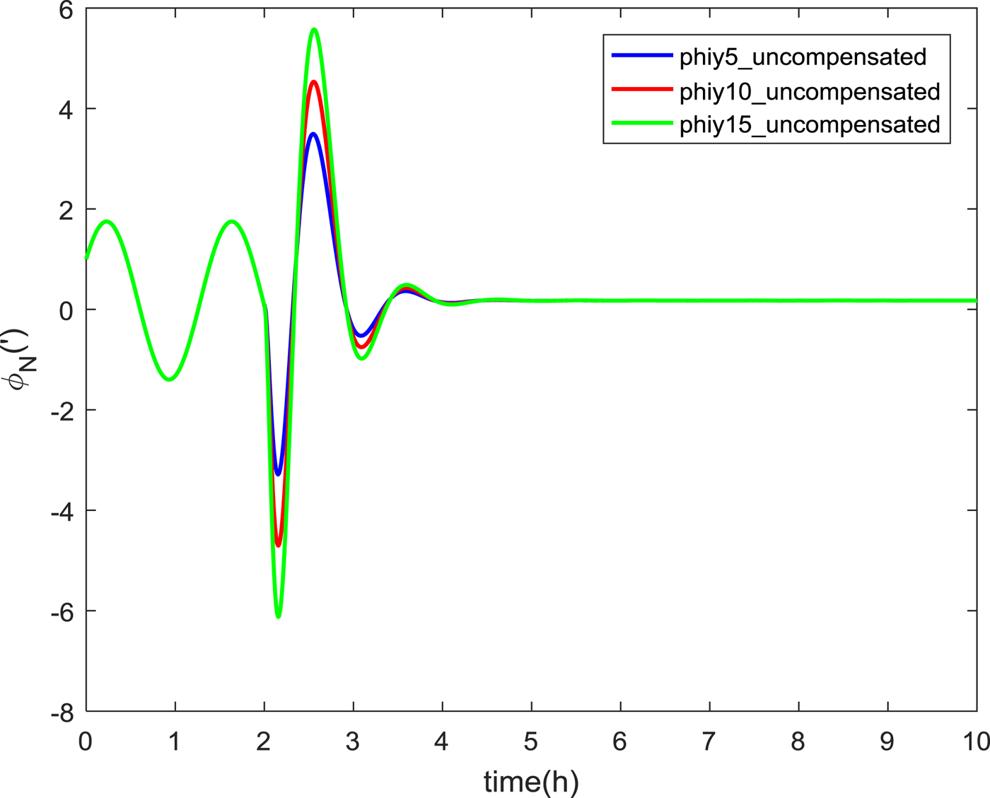
Figure 6. North misalignment angle at different speeds.
At time 2 h, the east output speed of the inertial navigation system was 21·68 m/s, 26·68 m/s and 31·68 m/s, respectively. The results show that the overshoot of the switching is proportional to the solution of the speed at the switching moment. After adding the switching compensation controller, the results for the north misalignment angle are shown in Figure 7.

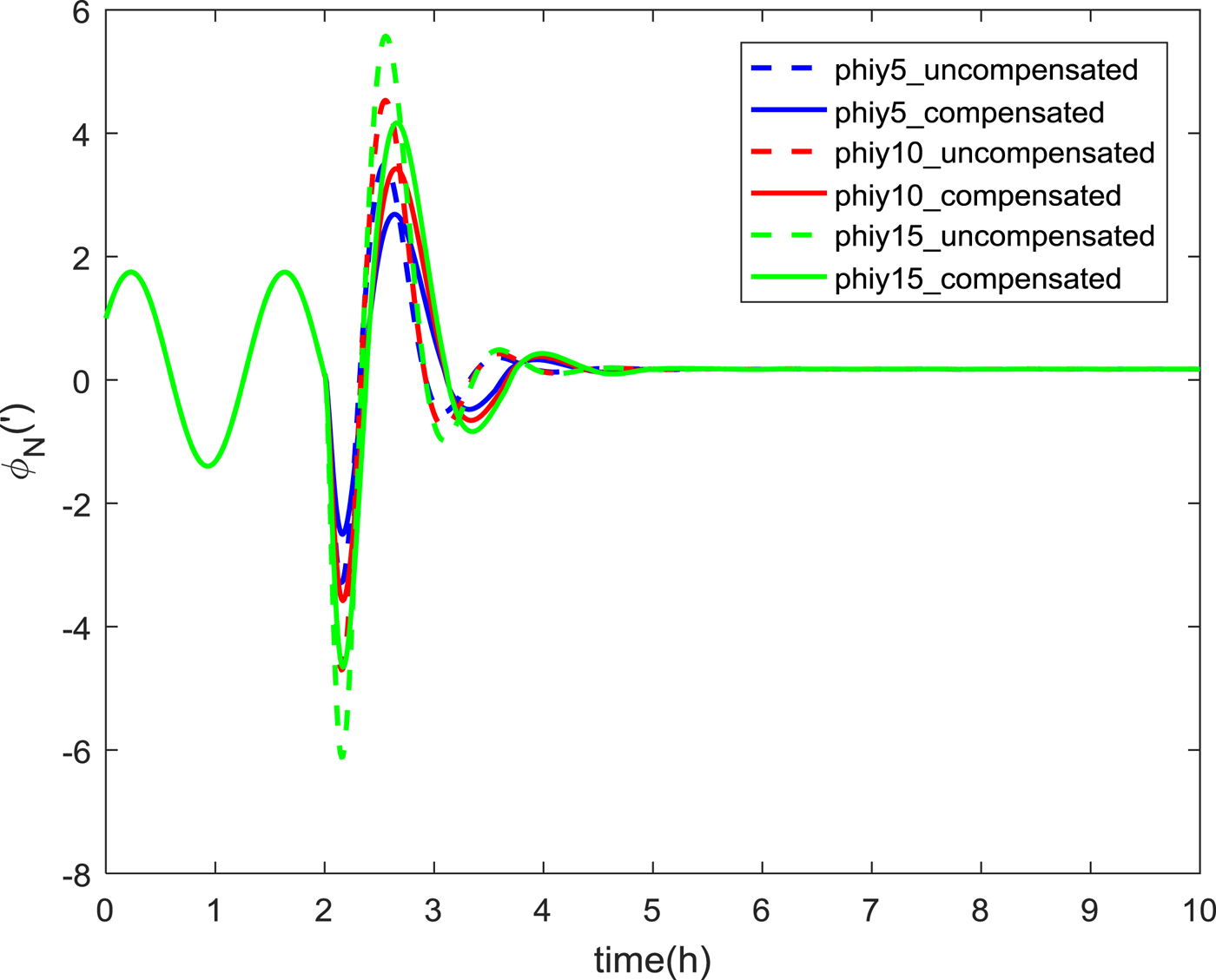
Figure 7. Comparison of north misalignment angles at different speeds.
As can be seen from Figure 7, the maximum overshoots of the north misalignment angles at 5 m/s, 10 m/s and 15 m/s without compensation were 3·49', 4·53' and 5·57', respectively. The maximum overshoot of the north misalignment angle with the switching compensation controller was 2·69', 3·43' and 4·16'. The accuracy was improved by 22%, 24% and 25%. It can be seen that the overshoot has obviously decreased after using the compensation controller. The greater the speed, the more obvious the effect.
6. CONCLUSION
A new switched control method for the damped and undamped switching problem has been proposed in this paper. A model of the switched control problem of inertial navigation system has been established. The average dwell time method was used to prove the exponential stability of the system. Sufficient conditions of exponential stability are given with constant disturbance and without disturbance. When the system is stable, the switching compensation controller is designed to reduce the overshoot. Significant results have been achieved. By properly adjusting the switching controller, the overshoot caused by the switching could be reduced further. This provides a theoretical basis for studying the optimal control problem under the condition of system stability and provides theoretical guidance for damped and undamped state optimal control of an inertial navigation system.
ACKNOWLEGEMENTS
This work was supported in part by the National Natural Science Foundation for Outstanding Youth (61422102) and Special Fund for Basic Research on Scientific Instruments of the National Natural Science Foundation of China (61127004).