


1. Introduction
The intermodal shipping container was invented by the American businessman Malcom McLean in 1956 (Levinson, Reference Levinson2006). Since then, containerisation has facilitated global trade by decreasing transportation time and costs. In 2018, the global volume of container cargo increased by 146⋅4 million twenty-foot equivalent units (TEU), and it has been forecasted to increase by 5% in 2021 (Knowler, Reference Knowler2019). It is undeniable that our daily lives cannot be sustained without container transportation as a global economic activity. Marine container transportation has enhanced the development of the global economy, and efficient and time-saving transportation has become a requirement in the past decades. Furthermore, the energy-efficiency design index (EEDI) has issued in the field of marine transportation since 2013. The reduction of greenhouse gas (GHG) emissions is required for marine container transportation to satisfy the EEDI.
Many studies on optimal ship routing have been conducted in the past decades (Bijlsma, Reference Bijlsma2008; Maki et al., Reference Maki, Akimoto, Nagata, Kobayashi, Kobayashi, Shiotani, Ohsawa and Umeda2011; Prpić-Oršić and Faltinsen, Reference Prpić-Oršić and Faltinsen2012; Shoji, Reference Shoji2013; Chang et al., Reference Chang, Tseng, Chu and Shao2016; Chou et al., Reference Chou, Chou, Hsu and Lu2017). These studies focused on the optimisation of the voyage time, fuel consumption and GHG emissions. However, during cargo operation and marine transportation, the internal air conditions of the container are influenced by changes in meteorological conditions, water content of the wooden container floor, cargo, packaging material and other external factors. When cargo is sealed in airtight containers, the moisture inside the container turns into condensation as a result of these changes. Water droplets formed by condensation inside the container cause serious damage to the cargo. Herein, a field survey of a Japanese container terminal was also conducted. It was observed that the moisture inside the wooden container floor influences the humidity inside the container. Iejavs and Rozins (Reference Iejavs and Rozins2016) evaluated the properties regarding the moisture permeability of cellular wood-panel walls with different thicknesses and weights. Chiniforush et al. (Reference Chiniforush, Valipour and Akbarnezhad2019) showed the effects of moisture content and temperature on the diffusion properties of glued laminated timber. Chang et al. (Reference Chang, Wi, Kang and Kim2020) assessed the moisture risk to cross-laminated timber based on different climate conditions, types of insulation and application of resistant materials. These studies showed that the moisture content of wooden materials varies with the type, thickness, weight and quality of the wood under different atmospheric conditions. All these factors contribute to the moisture inside a container. The condensation problem is simplified by considering the effects of external meteorological conditions only, because the measured results are available only for a dry box container with a plywood floor.
Studies on the issue of condensation in dry containers began in the 1970s (Imaeda et al., Reference Imaeda, Kubo, Hashimoto, Abe and Kiwaki1971). Weiskircher (Reference Weiskircher2008) summarised the results of six studies based on the effects of air temperature inside a dry container during its transportation through land and sea. This literature summarised the most important and significant research on condensation; however, little progress has been made in terms of further developments to address this problem. This can be attributed to the growing market share of reefer containers in early 2000. The market share of reefer containers under refrigerated transportation increased from 50% to 80% between 2005 and 2016, while that of the reefer vessels decreased from 50% to 20% (Castelein et al., Reference Castelein, Geerlings and Duin2020). In response to this growing trend, the focus of related studies has shifted from dry containers to reefer containers. In the case of reefer containers, the air condition can be regarded as a fluid dynamic problem to be addressed using computed fluid dynamics (CFD). However, the problem of condensation inside a dry container remains unsolved. Studies regarding this condensation problem and the air temperature in dry containers are discussed in the following paragraphs.
Ayyad et al. (Reference Ayyad, Valli, Bendini, Accorsi, Manzini, Bortolini, Gamberi and Gallina Toshi2017) studied the change in water content of vegetable oils when transported by two different types of containers. Their results showed that thermal isolation was effective in protecting cargo from climate stress. Sharp et al. (Reference Sharp, Fenner and Van Greve1979) tested the insulating ability of sugarcane fibre and aluminium foil when transporting cocoa beans from Papua New Guinea to Australia. Palacios-Cabrera et al. (Reference Palacios-Cabrera, Menezes, Iamanaka, Canepa, Teixeira, Carvalhaes, Santim, Leme, Yotsuyanagi and Taniwaki2007) examined the changes in the temperature, relative humidity and moisture content of green coffee beans transported from Brazil to Italy. The coffee beans in the hold showed the highest variation in moisture content, and the regions of the container near the wall and ceiling were found to be susceptible to condensation. Excell and Stone (Reference Excell and Stone1989) studied the condensation problem during the transportation of refined sugar in containers from Durban to Cape Town. They found that the hot sugar had greater probability of condensation than did the cold sugar, owing to the higher temperature gradient. These studies focus on evaluating the insulating ability of different materials from the viewpoint of condensation within the container. However, the internal conditions of these containers change with the external air conditions during marine transportation. The relationship between the internal and external air conditions was not discussed in these studies.
The climate profile inside containers has also been studied in the field of transportation and applied packaging. Leinberger (Reference Leinberger2006) performed experiments to measure extreme weather conditions by installing sensors inside containers for shipments between Asia, Europe and North America. Csavajda and Borocz (Reference Csavajda and Borocz2019) calculated the mean statistical value of the temperature and humidity inside containers for shipments from Hungary to India, China and South Africa. Borocz et al. (Reference Borocz, Singh and Singh2015) and Singh et al. (Reference Singh, Singh and Sandhu2012) highlighted the importance of special packaging design for protecting cargoes against extreme climate events during navigation. Accorsi et al. (Reference Accorsi, Manzini and Ferrari2014) measured the temperature variation inside a container during navigation from Italy to North America and Far East Asia. However, these studies did not focus on the meteorological conditions. In this study, we consider the meteorological conditions by conducting onboard measurements of outside air conditions in different seasons from Far East Asia to Europe. As it is not realistic to monitor the internal air conditions of all the containers, a new methodology should be modelled to estimate the internal air conditions from the external weather data. Meteorological conditions are measured onboard in different seasons from Far East Asia to Europe, and simple statistical models are constructed to estimate the internal air conditions of containers here.
In the field of heat conduction, Imaeda et al. (Reference Imaeda, Kubo, Hashimoto, Abe and Kiwaki1971), Imaeda and Kubo, (Reference Imaeda and Kubo1974) measured the changes in temperature and humidity inside and outside an aluminium container and an iron container in several ports in Japan. Although these studies attempted to investigate the relationship between the external and internal conditions of containers, the experiments were limited to land measurements.
In this study, we investigated the relationship between the inside and outside conditions of containers through sensor measurements of solar radiation, temperature and air temperature in a 20,000 TEU container ship travelling between Far East Asia and Europe in May 2019. We explored the mechanism of container condensation in different sea regions, seasons, latitudes and other factors on a time–space scale. Based on the measurements, we propose a statistical model to estimate the condensation probability by considering external weather conditions.
The rest of this paper is organised as follows. In Section 2, we describe the phenomenon of container condensation. In Section 3, we introduce the setting of the land and onboard measurements. In Section 4, we report and discuss the measurements and the results of a correlation analysis of each parameter. In Section 5, we describe the multi regression modelling and discuss the estimation results of the inside air conditions for all voyages. In Section 6, we define and estimate the condensation probability for certain patterns of loading and discharging ports. Finally, in Section 7, we present the conclusions of this study.
2. Definition of container condensation
In general, container condensation occurs if either one of the following conditions is satisfied:


where Tw [°C] = temperature of the internal side of the container wall at the top level, Di [°C] = dew point temperature inside the container, Ta [°C] = outside air temperature, and Da [°C] = outside dew point temperature. Case 1 occurs easily when the vessel is loaded at a port in a high-latitude region under cold weather conditions and is discharged at a port in a low-latitude region with warm weather conditions. During navigation from cold to warm regions, ${T_a}$ and ${D_a}$
 increase, while ${T_w}$
 remains almost the same in the case of poor ventilation; as a result, condensation may occur inside the container at the discharging port. Case 2 occurs easily when the vessel is loaded at a port in a low-latitude region with warm weather conditions and is discharged at port in a high-latitude region under cold weather conditions. During navigation from warm to cold regions, both ${T_a}$
 and ${D_a}$
 decrease, while ${D_i}$
 remains almost the same in the case of poor ventilation; as a result, condensation is expected to occur at the discharging port.
3. Land and onboard measurements
In this study, we first conducted land measurements of a real-scale container to examine the relationship between the air conditions inside and outside the container. Second, we conducted onboard measurements to study the weather changes during navigation across the ocean.
3.1 Land measurement
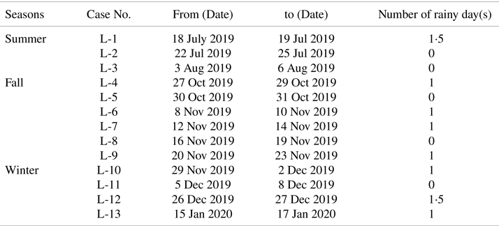
Land measurements were carried out at two different locations, as shown in Figure 1. First, measurements were carried out to determine the inside and outside air conditions, excluding solar radiation, of the real-scale dry box container shown in Figure 2 (left). The container was a 20-foot container (length: 6⋅058 m, width: 2⋅438 m, height: 2⋅591 m). The measurements were carried out at the Oshima National College of Maritime Technology in Yamaguchi, Japan, for several cases in summer (Cases L1–L3), fall (Cases L4–L9) and winter (Cases L10–13) in 2019 and 2020. The measurement programs are summarised in Table 1. The mounting positions of the sensors around the container are shown in Figure 2 (right). Inside the container, air temperature, humidity and condensation were measured at multiple positions (upper, middle and lower positions). Humidity inside the container was detected in the fall and winter seasons. Outside the container, the air temperature and humidity were measured simultaneously using thermocouples and thermohygrometers installed inside and outside the container, respectively. The condensation sensor is installed only for Case L-13. The measured data were recorded and transferred into a data logger every second. The solar radiation data measured by the Japan Meteorology Agency (JMA), Hiroshima, were used in this study. The weather conditions of Yamaguchi and Hiroshima were nearly the same because they are separated by only approximately 60 km.

Figure 1. Locations of measurements: Oshima National College of Maritime Technology in Yamaguchi and Japan Meteorological Agency (JMA) in Hiroshima, Japan
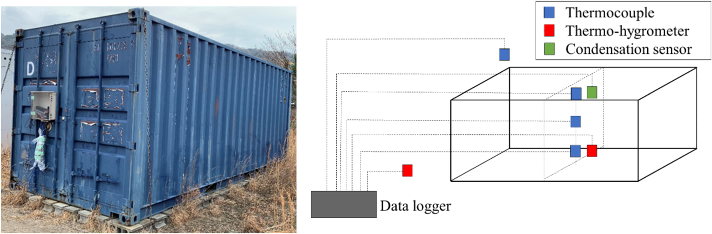
Figure 2. Photograph of the 20 ft dry box container used for the land measurements (left) and schematic of the setup of the land measurements and locations of sensors and data logger (right)
Table 1. Summary of the dates of the land measurements

Note: Condensation sensor is installed for only Case L-13.
The container used in the land experiment was leased in collaboration with a Japanese maritime organisation from the summer of 2019 to the winter of 2020. This rendered it difficult to carry out the land experiment during the spring season. The weather patterns of the spring season have been modified by applying the measured data from the fall season. Thus, future studies should ensure the accumulation of data during the spring season for more accurate results. The condensation inside a container is expected to occur empirically more in autumn, because the internal dew point temperature and humidity are more favourable for the formation of water moisture. Therefore, land experiments were frequently carried out in autumn over other seasons, to analyse the weather conditions facilitating condensation.
3.2 Onboard measurements during navigation
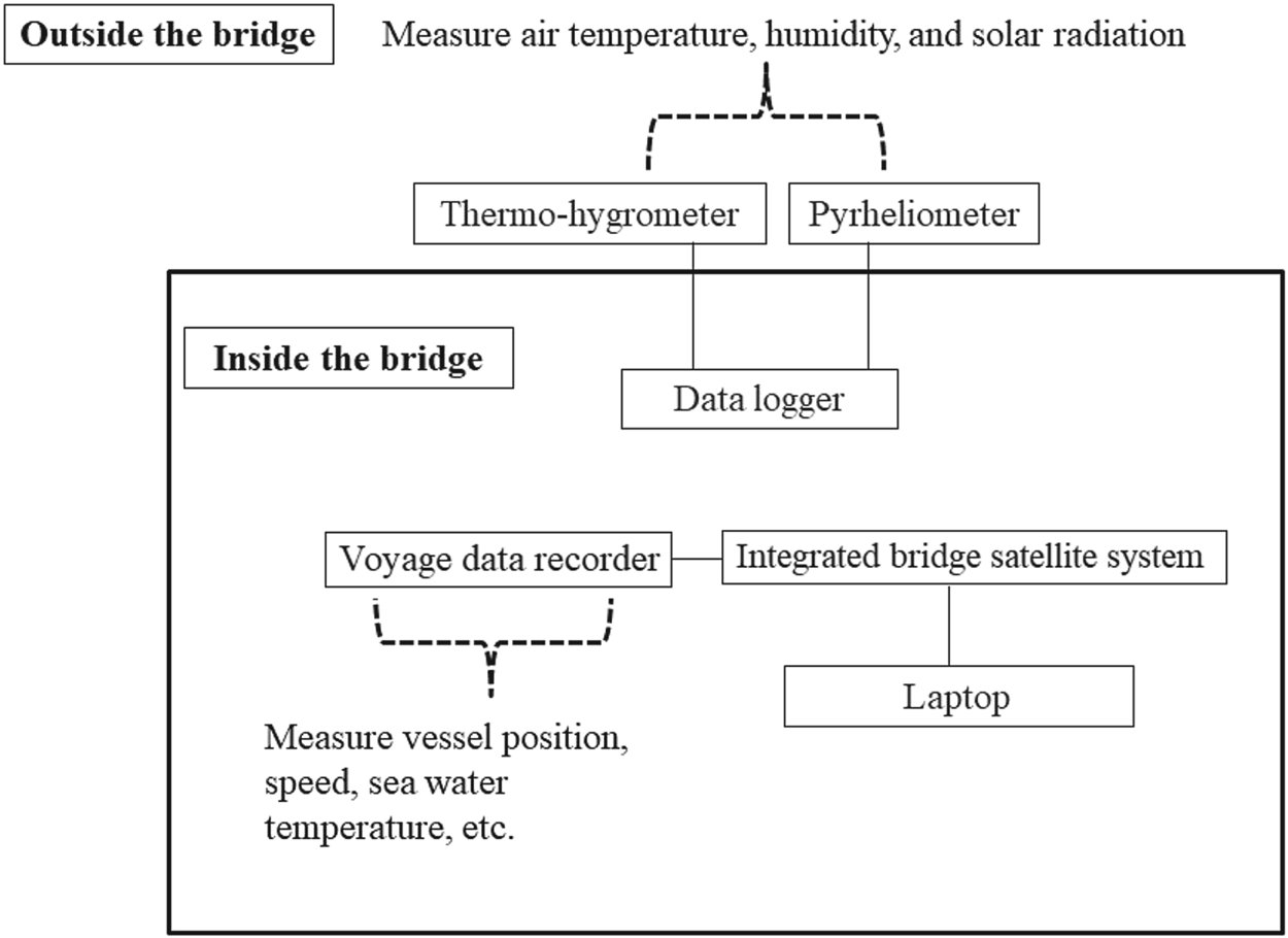
In the onboard measurements, it is ideal to install sensors inside for all the containers to monitor the situations during the voyage. However, this is not realistic, because the setting of nearly 20,000 sensors in each voyage seemed impossible for various reasons. Although onboard measurements were difficult owing to the technical problem of data transfer at sea, onboard monitoring techniques have been developed in recent decades (Sasa et al., Reference Sasa, Tereda, Shiotani, Wakabayashi, Ikebuchi, Chen, Takayama and Uchida2015, Reference Sasa, Faltinsen, Lu, Sasaki, Prpić-Oršić, Kashiwagi and Ikebuchi2017; Lu et al., Reference Lu, Sasa, Sasalo, Terada, Kano and Mizojiri2017; Jing et al., Reference Jing, Sasa, Chen, Yin, Yasukawa and Terada2021). In this study, we developed an onboard measurement system to monitor weather changes during the voyage on a newly built 20,000 TEU container vessel (see Figure 3) from May to December 2019. The vessel has a length of 400 m, breadth of 58⋅8 m, full loaded draft of 16⋅02 m and voyage speed of 22⋅8 knots.

Figure 3. Photograph of the 20,000 TEU container vessels used for the experiment
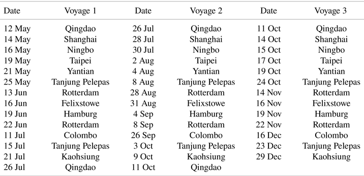
In container transportation, the main shipping routes are the Trans-Pacific, Trans-Atlantic and Asia–Europe routes. The voyage route of the 20,000 TEU container ship was between Far East Asia and Europe, as shown in Figure 4. The route went through the East China Sea, South China Sea, Indian Ocean, Red Sea, Mediterranean Sea and Atlantic Ocean, and it was connected with narrow waters, such as the Malacca Strait, Suez Canal, Gibraltar Channel and Dover Channel. The vessel completed three round trips between Qingdao, China, and Hamburg, Germany, from May to December 2019. The data measured on the vessel were collected at the end of December 2019 in Kaohsiung, Taiwan. Table 2 summarises all ports of call and visiting dates. Unlike the Trans-Pacific or Trans-Atlantic routes, this voyage route goes through many continents. Air conditions during navigation are influenced by the effects of reflection, absorption and radiation of heat, and these properties are much more complex in coastal areas than in the ocean. In other words, weather change is more sensitive near coastal regions. The measured weather parameters were the solar radiation, air temperature, humidity, sea water temperature and wind conditions, etc. A pyranometer and thermohygrometer were installed outside the bridge, which is the highest position of the vessel, as shown in Figure 5 (left and centre). The cables were connected from the sensors to the power supply and data logger inside the bridge. The measured data related to the navigation and engine were sent to the voyage data recorder, which must be installed for all outbound vessels. An integrated bridge satellite system connected to the voyage data recorder was also installed inside the bridge to establish communication from vessel to land. As shown in Figure 5 (right), a laptop was connected to the integrated bridge satellite system to collect navigation data, such as position, speed course, steering angle, wind speed and direction, which were recorded every second. The design of the onboard measurement system is illustrated in Figure 6.
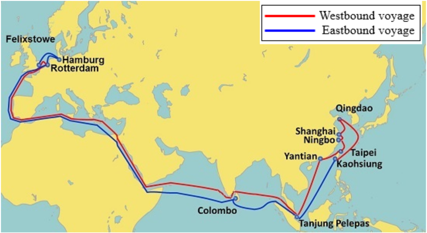
Figure 4. Voyage route of the container vessel. (Evergreen International Corp. Routing Network (2019))
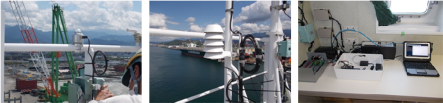
Figure 5. Photographs of the pyranometer (left), thermohygrometer (centre) outside the bridge and the devices for data storage inside the bridge (right)

Figure 6. Setup of the onboard measurement showing the locations of sensors and other recording devices inside and outside the bridge
Table 2. Summary of the ports of call for the three round trips in 2019

4. Land and onboard measurements results
4.1 Land measurement results
The results of the measurements of the air temperature, humidity (inside and outside), and solar radiation for Cases L-3 (summer), L-6 (fall) and L-12 (winter) are shown in Figures 79, respectively. The air temperatures inside the container are approximately 20–40°C higher than those outside the container in every season. The humidity outside the container increases from night to morning slightly more than the humidity inside the container. The maximum values of the solar radiation in summer, fall and winter were approximately 900, 600 and 420 W/m2, respectively.

Figure 7. Land measurements of air temperatures (inside and outside), humidity (outside) and solar radiation in summer (case L-3)
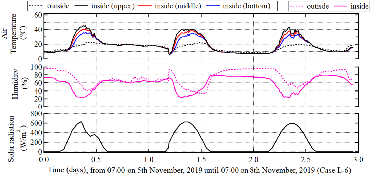
Figure 8. Land measurements of air temperatures (inside and outside), humidity (inside and outside) and solar radiation in fall (case L-6)
Figure 9. Land measurements of air temperatures (inside and outside), humidity (inside and outside) and solar radiation in winter (case L-12)
Figure 10 shows the maximum and minimum temperatures inside and outside the container in each season. The maximum air temperatures outside the container in Case L-3 (summer), Cases L-4 and L-5 (fall) and Case L-11 (winter) were 36, 25, 25 and 18°C, respectively. The highest air temperature inside the container was always measured in the upper position, and exceeded 50, 45 and 40°C in Case L-3 (summer), Cases L-4, 5, 6, 7, and 8 (fall), and Cases L-10 and 12 (winter), respectively. The minimum temperatures inside the container were comparable in all positions (upper, middle and bottom) and were 20, 8 and −1°C in summer, fall and winter, respectively.
Figure 10. Land measurements of maximum and minimum temperatures outside and inside the container (upper, middle and bottom parts)
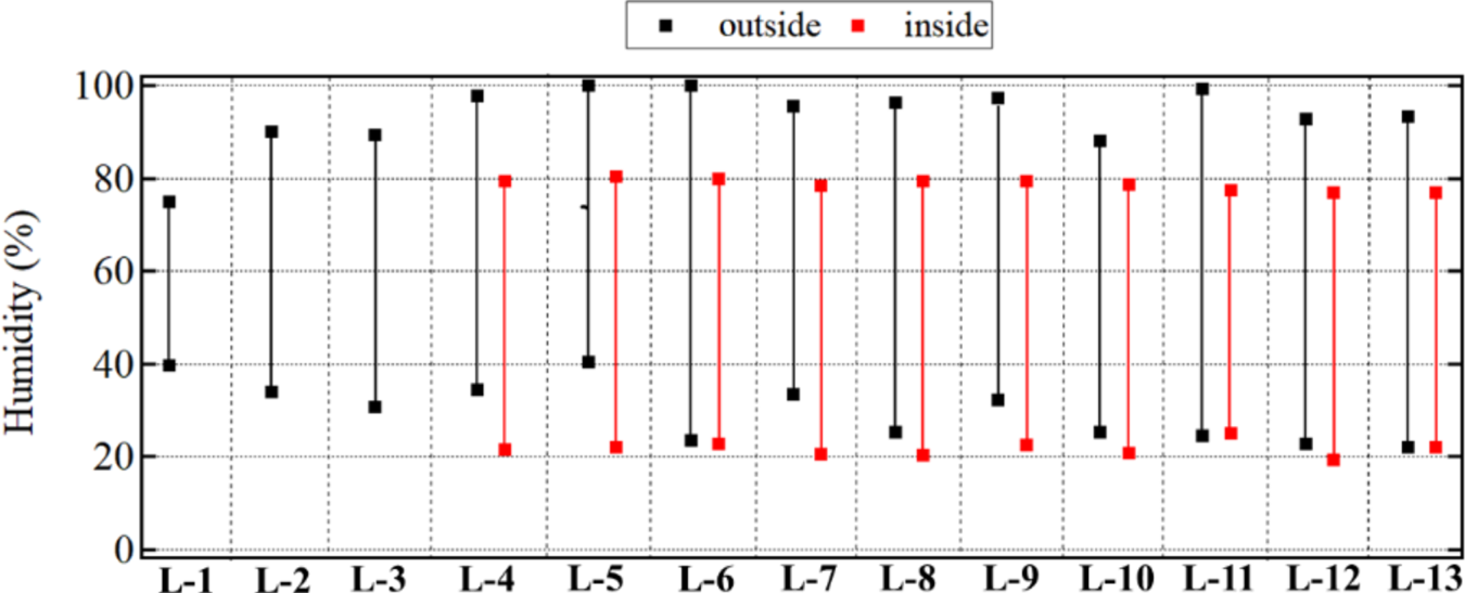
Figure 11 shows the measurement results of the maximum and minimum humidity inside and outside the container in each season. The maximum and minimum humidity inside the container were approximately 80% and 20%, respectively, in Cases 4–12 (fall and winter). This trend was not observed in summer owing to data unavailability. It can also be seen that the humidity outside the container was 10%–20% higher than that inside the container. Furthermore, the minimum humidity outside the container in summer was slightly higher than those in fall and winter.

Figure 11. Land measurements of maximum and minimum humidity outside and inside the container
4.2 Onboard measurement results
In the westbound route, the ship departs from Qingdao, China, (Day 1) at 36°N, passes through the Malacca Strait (Day 13) at 01°N, and arrives in Hamburg, Germany, (Day 40) at 56°N. Then, the eastbound voyage starts from Europe to China on Day 40 and ends on Day 80. Figure 12 shows the latitudes for each voyage. The figure shows that the maximum difference in latitude is 55°; owing to this large latitude difference, a significant variation in air conditions is expected over the 40-day voyage.
Figure 12. Latitudes of voyages 1–3
4.2.1 Calculation of dew point temperature during navigation
As mentioned in Section 2.1, we assumed that condensation occurs if Equation (1) or (2) is satisfied. The dew point temperature can be calculated from the air temperature Ta [°C] and relative humidity R.H. [%] as

where ${P_w}$ [kPa] = vapor partial pressure, and ${P_{ws}}$
 [kPa] = saturation vapor pressure, which is a function of the temperature. Among the various equations proposed to calculate ${P_{ws}}$
 (Goff, Reference Goff1957; Murray, Reference Murray1967; Buck, Reference Buck1981; Alduchov and Eskridge, Reference Alduchov and Eskridge1995), Tenten's equation is the most frequently used (Verhoef et al., Reference Verhoef, Diaz-Espejo, Knight, Garcial and Fernandez2006; Gao et al., Reference Gao, Brewster and Xue2008):

Substituting Equation (4) into Equation (3) and rearranging the formula, the dew point temperature ${T_{dp}}$ [°C] can be expressed as

where A = coefficient calculated by

Air temperature, humidity and direct sunlight can be considered as the primary factors influencing the internal air conditions of the container. The relationship of these factors with condensation was analysed, as described in the following section. Sea water temperature was also included in the analysis because of its close relationship with the air temperature. The comparison of these factors helps to develop a good understanding of how air temperature changes with sea water temperature in an actual sea. Although the sea water temperature also influences the air conditions of containers stowed in a cargo hold, sufficient data regarding the distribution of air temperatures or solar radiation have not been collected, which must be considered in future studies.
4.2.2 Air temperature, sea water temperature and dew point temperature
Figure 13 shows the air temperature, sea water temperature and dew point temperature measured in Voyages 1–3. The dew point temperature in the outside air was calculated using Equations (5) and (6) based on the outside air temperature and humidity. The difference in air temperature was approximately 15°C between Qingdao and the Indian Ocean (Days 1–10) in Voyage 1 (spring) and Voyage 3 (fall). However, in Voyage 2, the air temperature was maintained at approximately 30°C on Days 1–20 (summer). This implies that the seasonal difference in air temperature becomes greater and more significant at higher latitudes. On the other hand, the air temperature remains almost constant throughout the year in tropical regions, such as the Indian Ocean. The air temperature is slightly lower in Voyages 2 and 3 than in Voyage 1 over the Indian Ocean. The measured data show that the air temperature was approximately 30°C when the ship passed through the Indian Ocean on Days 13–21 and 57–67 in Voyages 1–3. The air temperature was constant until the ship passed through the Suez Canal (Days 20–25) in each case. Over the Mediterranean Sea, the air temperature drops significantly towards the Gibraltar Channel and the Atlantic Ocean. The difference in air temperature is approximately 15–25°C from the Mediterranean Sea to the Atlantic Ocean (Days 23–32 and Days 46–55). The difference in temperature between Europe and the Indian Ocean tends to increase in Voyage 3 (winter) compared to Voyages 1 and 2. It is obvious that the ship encounters two significant changes in air temperatures over long periods of approximately 10 days, and this change in meteorological conditions can influence container condensation. In addition, some large, short-period variations of around one day were observed on Days 25–55. It is also shown that the sea water temperature is similar to the air temperature during most of Voyages 1–3, except on Days 35–50 (Europe) in Voyages 2 and 3. This implies that the long-period variations in air temperature and sea water temperature are strongly related to each other. The dew point temperature of the outside air is 2–5°C lower than the air temperature in all the voyages.

Figure 13. Onboard measurements of air temperature, sea water temperature and dew point temperature in voyages 1–3
4.2.3 Solar radiation
Figure 14 shows the variation in solar radiation in Voyages 1–3. In the Indian Ocean (Days 13–21 and Days 57–67), in all voyages, although low levels of solar radiation are expected during rainy or cloudy days, only negligible variation was generally observed at low latitudes. The maximum values of solar radiation in the Indian Ocean in Voyages 1–3 were 1,000–1,200 W/m2. In contrast to the Indian Ocean, a remarkable decrease in solar radiation was observed over Europe and Far East Asia. Over Europe (Days 35–50), the maximum values of solar radiation in Voyages 1, 2 and 3 were 1,020, 900 and 220 W/m2, respectively. In Far East Asia (Days 1–10 and 67–80), the maximum values of solar radiation in Voyages 1, 2 and 3 were 1,040, 1,100 and 900 W/m2, respectively. Although the decrease over Far East Asia in Voyage 3 is not significant compared to that over Europe, the solar radiation tends to decrease more significantly during the winter season in higher-latitude regions. In particular, the solar radiation may influence the long-term variations in air temperature and sea water temperature.

Figure 14. Onboard measurements of solar radiation in voyages 1–3
4.2.4 Humidity and water vapor pressure
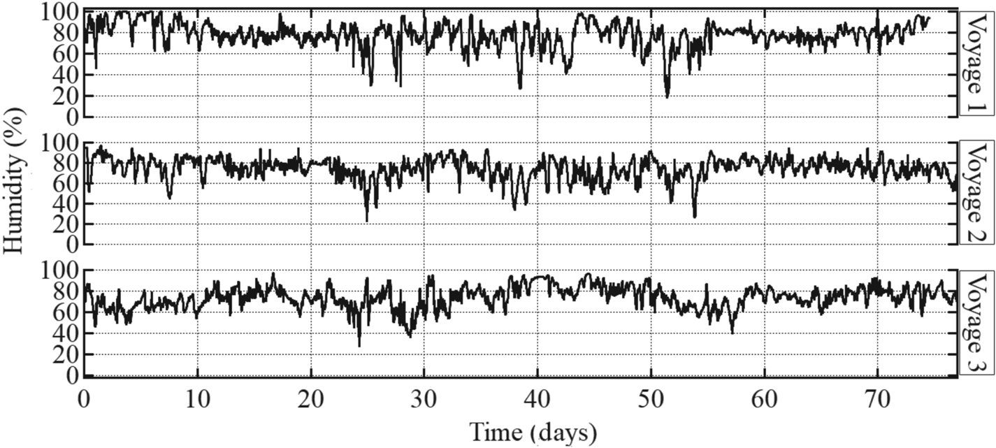
Figure 15 shows the measurements of the humidity in Voyages 1–3. Over the Indian Ocean (Days 13–21 and 57–67), humidity was maintained at approximately 60%–90%. On the other hand, a humidity of more than 95% was measured in Europe (Days 35–50) in Voyages 1 and 3 and in Far East Asia (Days 1–10 and Days 67–80) in Voyages 1 and 2. In addition, significant short-term variations were observed in Europe and Far East Asia. In Europe, the largest daily variations were found to be from 24% to 90% and from 38% to 80% in Voyages 1 and 2, respectively. In Far East Asia, the largest daily variations were found to be from 42% to 98% and from 42% to 88% in Voyages 1 and 2, respectively.

Figure 15. Onboard measurements of humidity in voyages 1–3
Figure 16 shows the water vapor pressure in Voyages 1–3 calculated using Equations (5) and (6) based on the air temperature and humidity measurements. A higher humidity is measured over Europe than the Indian Ocean, while the water vapor pressure shows the opposite trend. The water vapor pressure over the Far East Asia and the Indian Ocean was approximately 2 and 3 kPa, respectively, in all voyages. However, in Europe, the water vapor pressure decreased from approximately 1⋅5 to 0⋅5 kPa from Voyage 1 to Voyage 3. This shows that the water vapor pressure in Europe decreases obviously from summer to winter. This also indicates that the water vapor content may be higher at lower latitudes than at higher latitudes. These results indicate that the water vapor pressure changes more in a long period than humidity. Although humidity is higher at higher latitudes, this tendency is not strong. Because the water vapor pressure is an indicator of the actual moisture content in the air, it was selected for the estimation of the condensation in this study.

Figure 16. Calculation results of water vapor pressure in voyages 1–3
4.3 Statistical analysis of measured parameters
4.3.1 Correlation analysis of land measurements
A correlation analysis was conducted to determine the relationship between the outside and inside air conditions. Figures 17–19 show plots of the inside temperature as a function of the solar radiation, outside temperature and outside humidity, respectively. The absolute values of the correlation coefficient are found to be approximately 0⋅8–0⋅9, indicating strong relationships. Figure 20 shows plots of the inside temperature as a function of the outside water vapor pressure. The absolute values of the correlation coefficient in each season are found to be approximately 0⋅10–0⋅49. In summer, the water vapor pressure varies around 1⋅5–3⋅4 kPa, and the inside temperatures tend to increase when the outside water vapor pressure decreases. This tendency is not clearly observed in fall and winter; the variation in water vapor pressure decrease to approximately 0⋅5–1⋅5 kPa in fall and 0⋅5–1⋅0 kPa in winter.
Figure 17. Relations of inside temperature as a function of the solar radiation in summer (left), fall (middle) and winter (right)

Figure 18. Relations of inside temperature as a function of the outside air temperature in summer (left), fall (middle) and winter (right)

Figure 19. Relations of inside temperature as a function of outside humidity in summer (left), fall (middle) and winter (right)
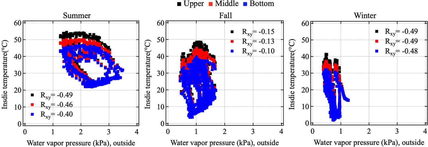
Figure 20. Relations of inside temperature as a function of outside water vapor pressure in summer (left), fall (middle) and winter (right)
4.3.2 Correlation analysis of onboard measurements
The outside air conditions vary significantly because the ship moves across different sea areas with large differences in latitude (55°) between the Malacca Strait and the Port of Hamburg, Germany. Figure 21 shows plots of the air conditions as functions of the latitude. The correlation coefficients are found to be −0⋅80, −0⋅77 and −0⋅93 in Voyages 1, 2 and 3, respectively. This shows that the air temperature is strongly influenced by the position of the ship, especially the latitude. The air temperature showed little change at low latitudes (0–15°N, Indian Ocean). On the other hand, it varied significantly at latitudes higher than 40°N, especially in Voyage 3. Furthermore, it is worth noting that the water vapor pressure shows a similar variation with the air temperature, with high correlation coefficient of −0⋅84, −0⋅77 and −0⋅95 in Voyages 1, 2 and 3, respectively. On the other hand, the solar radiation and humidity are less correlated with the latitude than with the air temperature and water vapor pressure. However, it suddenly dropped at 30°N near the Red Sea and the Suez Canal. A similar phenomenon was observed at 53°N near the Port of Hamburg, Germany. It is worth noting that the former case occurs in coastal areas and the latter occurs in an inland port. This indicates that the air condition is sensitive because different values of thermal capacity in land and sea influence each other, as mentioned in the field of meteorology (Kondo, Reference Kondo2004).
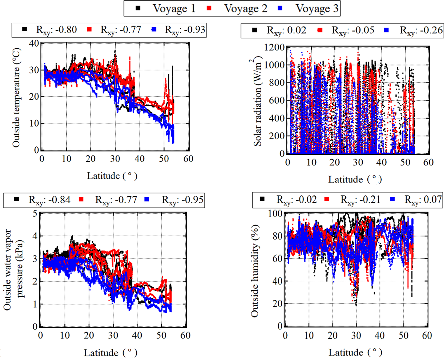
Figure 21. (top-left) outside temperature, (top-right) solar radiation, (bottom-left) outside water vapor pressure and (bottom-right) outside humidity as functions of the latitude in voyages 1–3
5. Multi-regression modelling and estimation results
5.1 Multi-regression modelling
The air temperature and water vapor pressure inside the container were estimated with multi-regression models. Equation (7), defined as Model I, shows that multi-regression formulae consist of three explanatory variables, ${x_1}$ , ${x_2}$
 and ${x_3}$
 , which represent the external air temperature, external water vapor pressure and solar radiation in this study, respectively; ${T_1}, {T_2},$
 and ${T_3}$
 denote the air temperatures inside the container at the upper, middle and bottom locations, respectively; ${W_p}$
 is the water vapor pressure inside the container, and ${\beta _0}, {\beta _1}, {\beta _2}$
 and ${\beta _3}$
 are the corresponding regression coefficients. The accuracy of Model I was the highest, so the other models were not used in this study.

5.1.1 Data adjustment for summer season
Before the multi-regression analysis, the following data adjustments were made. First, the data measured on rainy days (see Table 1) were excluded because the patterns of rain are complicated and reduce the estimation accuracy. The results of the land experiment included data for some rainy days, and it is difficult to model such conditions because of the limited amount of data. The percentage of sunny days was dominant in three voyages between the Far East Asia and Europe in 2019. Thus, the statistical models were constructed by excluding the rainy days in the land experiment. Second, the data are adjusted in Cases L1–L3 (summer) because the land measurement is not continuously conducted throughout the year, and there is a time gap of three months between the summer and fall seasons. Hence, data measured on 28 October 2019 (Case L-4), which is the earliest measurement in fall, were added to adjust the time period of the summer season to fill this time gap. We believe that this adjustment of data was necessary because no land experiments were carried out in September. To reflect the change in the weather conditions from August to September, the method of data supplement was used.
5.1.2 Regression modelling of inside air temperatures and inside water vapor pressure
Figure 22 shows the coefficient of determination R 2 results with regression Model I for the inside air temperature (upper level) and inside water vapor pressure. Other R 2 values of the inside air temperatures (middle and bottom levels) are not shown here because they are like those in the upper level. The figure illustrates that Model I had the highest R 2, with values of 0⋅96, 0⋅94 and 0⋅88 in summer, fall and winter, respectively. This indicates that estimation should be conducted using three explanatory variables.

Figure 22. R 2 of model I for the inside air temperature and inside water vapor pressure
Regression models for water vapor pressure show similar trends to those for the inside air temperature. The R 2 values of Model I were 0⋅95 and 0⋅81 in fall and winter, respectively. In Model I, the inside air temperatures and water vapor pressure in summer, fall and winter were calculated using Equations (8)–(10), respectively.


5.2 Estimation of inside air conditions during navigation
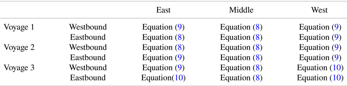
Air conditions inside each container during navigation were estimated using multiple regression formulas. It has been shown that three parameters (outside air temperature, outside water vapor pressure and solar radiation) strongly influence the air conditions inside the container. However, the solar radiation and outside air temperature of the container are different at different locations on the ship because they depend on the direction of sunlight. In onboard measurements, outside air conditions were measured only on the bridge of the ship. Considering these facts, the condensation is discussed for containers with direct solar radiation, i.e., at the highest position, left-most and right-most positions on the deck. According to the Köppen–Geiger climate classification (Kottek et al., Reference Kottek, Grieser, Beck and Rudolf2006), the world map can be classified into different climate regions based on the global temperature and precipitation data sets. Based on this classification, the voyage route of the container ship between China and Europe can be divided into six different climate regions. To fully apply this classification, it was necessary to conduct the land experiments in each of these climate regions. However, in this study, land experiments were only carried out in Japan, owing to the large spatial scale and a limited budget; therefore, a simplified classification was applied by dividing the voyage into three different regions (east, middle and west), as shown in Figure 23. In this simplified classification, the Indian Ocean and South China Sea both belong to the equatorial climate region and can therefore be defined as the middle region. On the other hand, the Mediterranean Sea, Atlantic Ocean and Europe exhibit a similar characteristic of warm temperate climate and can therefore be defined as the west region. Finally, considering the latitude and temperature difference, the East China Sea can be regarded as the east region, despite a similar climatic classification to that of Europe in this study. Table 3 summarises the regression equations used for each region. In the east region, Equation (9) was applied to the westbound Voyage 1 (spring) owing to the lack of a spring regression model.

Figure 23. Definition of the east, middle and west regions of the voyage
Table 3. Selections of regression equations for parameter estimation during navigation

The estimated results of the inside air temperatures in Voyages 1–3 are shown in Figures 24–26, respectively. Figure 27 shows the inside temperature difference between the upper and bottom levels for all voyages. Figure 28 shows the outside humidity and the estimated inside humidity for all voyages. The inside humidity was obtained from the inside temperature (upper level) and inside water vapor pressure estimated using Equations (3) and (4), respectively; the inside dew point temperature was obtained from the inside humidity and inside air temperature in the upper level estimated using Equations (5) and (6), respectively.

Figure 24. Variations in the estimated inside temperatures, dew point temperature and humidity in voyage 1

Figure 25. Variations in the estimated inside temperatures, dew point temperature and humidity in voyage 2

Figure 26. Variations in the estimated inside temperatures, dew point temperature and humidity in voyage 3
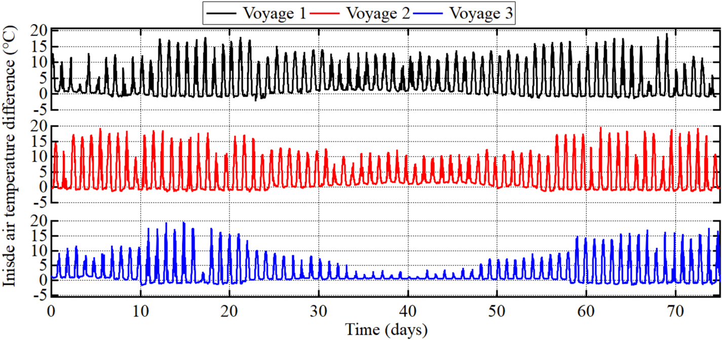
Figure 27. Variations in the inside air temperature difference between upper and bottom level in all voyages

Figure 28. Variations in the estimated inside and outside humidity in all voyages
5.2.1 Estimated inside air temperatures and dew point temperatures
Figures 24 and 26 show that the maximum inside air temperature (upper level) increases from approximately 45–60°C when the ship passes from Far East Asia to the Indian Ocean (Days 1–21) in Voyages 1 (spring) and 3 (fall). However, as shown in Figure 25, it remains between approximately 55 and 62°C in Voyage 2 (summer). The maximum inside temperature (upper level) increases even more when the ship navigates from the Indian Ocean to the Mediterranean Sea with a large difference in latitude. The difference of the maximum inside air temperature (upper level) between the middle and west regions is approximately 15°C in Voyages 1 and 2. However, it increased to approximately 35°C in Voyage 3. These results indicate that the latitude and season influence the inside air temperatures. The inside air temperatures change particularly when the ship navigates from low latitudes, such as the Indian Ocean, to high latitudes, such as Europe, in the winter season. It is worth noting that the inside air temperature (upper level) increased to almost 70°C when the ship travelled across coastal seas near the Suez Canal, and to almost 60°C inland ports of Europe in Voyage 1. The daily variation in the dew point temperature was approximately 12°C in the middle region in all the voyages and in the east region in Voyage 2 (summer). However, this variation decreased at high latitudes. In Europe, the daily variation was only approximately 5°C in all voyages. Furthermore, the inside air temperatures were almost the same as the dew point temperature in Voyage 3 (winter) in Europe. This indicates that there is a high probability of container condensation during that time period. It can be observed that latitudes and seasons also influence the difference in the inside air temperatures between the upper and bottom levels, as shown in Figure 27. The difference is approximately 15–20°C in all the voyages when the ship is in the Indian Ocean (Days 13–21 and Days 57–67). However, the difference decreases at higher latitudes. In Europe (Days 35–50), the difference in Voyages 1, 2 and 3 is approximately 12, 10 and 2°C, respectively. In Far East Asia (Days 1–10 and 67–80), the difference is like that in the Indian Ocean in Voyage 2 (summer), but it decreased to 2–10°C in Voyages 1 (spring) and 3 (fall).
5.2.2 Estimated inside humidity
As shown in Figure 28, the inside humidity is also influenced by the latitude and season. First, the inside humidity tends to be higher at higher latitudes. When the ship travels across the Indian Ocean (Days 13–21 and 57–67), the maximum humidity remains approximately 70%–80% in all voyages. However, it increases to 95%–100% when the ship is in Europe (Days 35–50) in Voyages 1 and 2. The inside humidity in Europe during winter in Voyage 3 is higher than in Voyages 1 (summer) and 2 (fall). During Days 35–50, the humidity reaches 95%–100% after approximately 1, 1⋅3 and 8 days in Voyages 1–3, respectively. In Far East Asia (Days 1–10 and 67–80), the inside humidity remains approximately 90% in Voyage 1 (spring) and decreases to approximately 70%–80% in Voyages 2 (summer) and 3 (Fall). This tendency is like that of the outside humidity discussed in Section 4.2.
5.2.3 Comparison of estimated results with land measurement
In this section, we compare the inside air conditions estimated by the multi-regression model with the land measurements. As reported in Section 4.1, the inside air temperature (upper level) measured on land in summer, fall and winter is approximately 55, 40 and 38°C, respectively. The results obtained using Equations (8) and (9) are similar to these land measurements. However, in Europe (Voyage 3), the estimated inside air conditions are very different from the land measurements in winter owing to the higher latitude. The estimated inside temperatures using Equation (10) are smaller than those for the land measurements. The difference in the inside air temperature (upper level) over Europe and on land in winter is approximately 20°C. In addition, a significant difference between Europe and the land measurements was observed in the estimated inside humidity, which varied within approximately 20%–80% in fall and winter, as reported in Section 4.1. However, the estimated humidity was more than 95% according to Equations (9) and (10) for all voyages in Europe. On the other hand, the estimated results and measurements were similar in the Indian Ocean, Far East Asia and on land (Japan) in all voyages.
6. Calculation of condensation probability
6.1 Definition of condensation inside the container and condensation probability
As mentioned in Section 2, condensation may occur inside the container if either of the following conditions is satisfied: ${T_w} < {D_a}$ and ${D_i} > {T_a}$
 . These conditions were checked with land measurements. Figure 29 shows the outside humidity, inside air conditions and periods of condensation inside the container. In this paper, the difference between the inside air temperature ${T_1}$
 (upper level) and the inside dew point temperature ${D_i}$
 is defined as ${T_d}$
 . Condensation occurs when the inside humidity exceeds 70% and ${T_d}$
 decreases below 8°C. Based on these results, the condensation conditions can be summarised as


where ${H_i}$ = inside humidity. The condensation probability, ${P_{\textrm{con}}}$
 , in the actual sea is defined as

where ${T_{\textrm{con}}}$ = period that satisfies Equations (11) and (12), and ${T_{\textrm{toal}}}$
 = voyage time from the loading port to the discharging port.
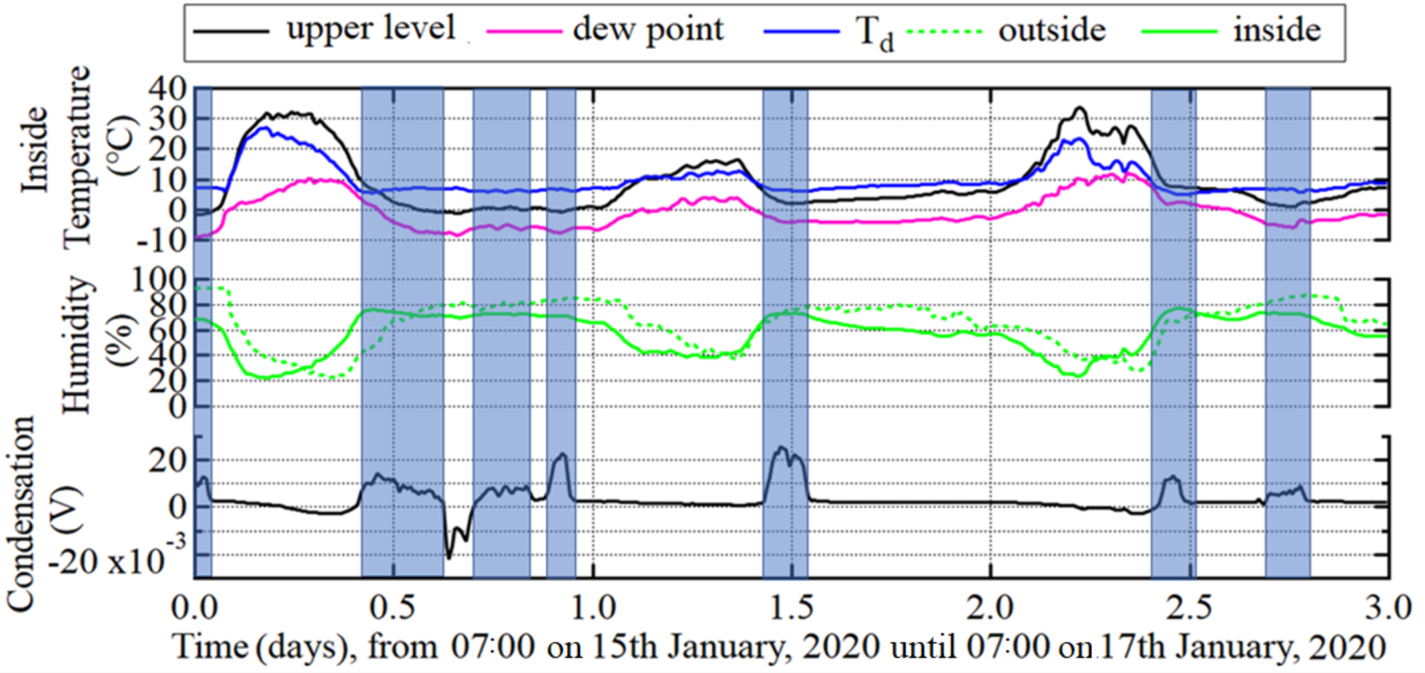
Figure 29. Variations in the inside air temperature, outside humidity and condensation measured on land (L-13). (Note: blue area is the period of condensation.)
6.2 Calculation of condensation probability during navigation
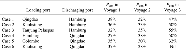
The probability of condensation, ${P_{\textrm{con}}}$ , is estimated using Equation (13) for certain patterns of the loading and discharging ports. The estimated results of ${P_{\textrm{con}}}$
 are presented in Table 4, where Cases 1–3 refer to westbound voyages and Cases 4–6 refer to eastbound voyages. Figure 30 show the relationship between the latitude and ${P_{\textrm{con}}}$
 in Cases 1 and 4, respectively. As shown in Figure 30 (left), ${P_{\textrm{con}}}$
 increase steadily to 10%–20% in all the voyages when the ship travels from 36°N–0°. It then reaches 22%–25% before the ships enters the Dover Channel at approximately 49°N. In Voyages 1 and 2, ${P_{\textrm{con}}}$
 increased to 38% and 32%, respectively, while in Voyage 3, it increased significantly from approximately 25% to 47% when the ship travelled at high latitudes in Europe. In Cases 2 and 3, ${P_{\textrm{con}}}$
 was 50%–55% in Voyage 3, indicating that the ship may experience container condensations for nearly half of the total voyage time in the westbound voyage in winter, regardless of the loading ports. In Case 4 (Hamburg, Germany, to Qingdao, China), ${P_{\textrm{con}}}$
 in Voyages 1, 2 and 3 was estimated to be 27%, 38% and 50%, respectively. As shown in Figure 30 (right), after the ship departs from Europe, ${P_{\textrm{con}}}$
 increases to approximately 18%, 32% and 45% from 54°N–0° in Voyages 1, 2 and 3, respectively. Then, ${P_{\textrm{con}}}$
 increases by only 5%–10% in all voyages when the ship arrives at Qingdao, China. This indicates that the risk of condensation is higher during winter (Voyage 3) than during summer and fall (Voyages 1 and 2). In Case 5 (Colombo, Siri Lanka, to Qingdao, China), ${P_{\textrm{con}}}$
 was 30%–35% in all voyages. In Case 6 (Kaohsiung, Taiwan, to Qingdao, China), ${P_{\textrm{con}}}$
 decreased from 37% to 28% in Voyages 1 and 2. As shown in Figure 30 (right), the estimated inside humidity in Voyage 1 was approximately 70%–80% on Days 70–75 and remained constant at approximately 70% in Voyage 2 during the same period. Thus, ${P_{\textrm{con}}}$
 in Case 6 is estimated to be higher in Voyage 1 than in Voyage 2. The estimated ${P_{\textrm{con}}}$
 in Case 3 (Voyage 3) is not shown here because we only had measurements until Kaohsiung, Taiwan. ${P_{\textrm{con}}}$
 is similar in westbound Voyages 2 and 3 and is slightly different in Voyage 1. On the other hand, ${P_{\textrm{con}}}$
 is very different in all eastbound voyages. In the westbound voyages, ${P_{\textrm{con}}}$
 increases by only 5%–7% in all voyages from 0° to 35°N. However, in the eastbound voyages, ${P_{\textrm{con}}}$
 increases by approximately 5%, 20% and 25% in Voyages 1, 2 and 3 from 35°N to 0°, respectively. This indicates that the probability of condensation is highest when the ship passes through the Indian Ocean and Mediterranean Sea and when the containers are loaded at higher latitudes, such as Europe, especially in fall and winter.

Figure 30. Condensation probability ${P_{\textrm{con}}}$ as a function of the latitude in case 1 (Qingdao, China to Hamburg, Germany) (left) and case 4 (Hamburg, Germany to Qingdao, China) (right) in the different voyages
Table 4. Condensation probability ${P_{\textrm{con}}}$ in different loading and discharging ports
7. Conclusions
This study is defined as the first step to investigate the condensation within a dry box container by proposing a simple method. Simultaneously, onboard data are being collected presently to investigate the distribution of heat and temperature of each container for further studies. The main conclusions of this study are as follows.
(1) The land measurements revealed that the inside humidity does not vary significantly in fall and winter, and the air temperatures and solar radiation have significant variations throughout the year.
(2) The outside air conditions during navigation show complicated patterns owing to the large differences in latitude and the different meteorological conditions. This causes significant changes in outside air temperature, humidity and solar radiation, especially during the winter season.
(3) In land, the inside temperature (upper level) was highly correlated with the solar radiation (rxy = 0⋅92), outside air temperature (rxy = 0⋅86) and outside humidity (rxy = −0⋅88). During navigation, the latitude was highly correlated with the outside air temperature (rxy = −0⋅80) and the water vapor pressure (rxy = −0⋅84).
(4) During navigation the water vapor pressure has a higher correlation with latitude than the humidity for the voyage route between Far East Asia and Europe. Hence, the outside water vapor pressure should be evaluated as a parameter in multi-regression analysis.
(5) It is shown that the inside air conditions should be estimated by the model with the following three explanatory variables: outside air temperature, water vapor pressure and solar radiation.
(6) In land, condensation is found to occur if the absolute difference between the dew point temperature and air temperature inside the container is smaller than 8°C and the inside humidity is higher than 70%. These conditions were applied to estimate the condensation probability for all voyages. The condensation probabilities are the highest in winter (Voyage 3), with a value of 47% and 50% in the westbound and eastbound voyages, respectively. This implies that the ship may encounter the air condition of condensation for almost half of the total period in containers with direct solar radiation.
(7) It was shown that the condensation probability remains at approximately 50% in Cases 1–3 during the winter season, especially in the westbound route, regardless of the loading ports. However, the condensation probability is lowered by 10%–20% if the container is loaded at lower latitudes, e.g., in Colombo, Sri Lanka, and Kaohsiung, Taiwan, in Cases 5 and 6 (Voyages 2 and 3).
(8) In the westbound voyages, variations of condensation probability were similar between Voyages 2 and 3 and were slightly different in Voyage 1. In the eastbound voyages, variations were very different in all voyages. The risk of condensation increased by 15%–20% when the ship passed through the Mediterranean Sea and the Indian Ocean and when containers were loaded at higher latitudes, such as Europe.
(9) The results of study show that container condensation is likely to occur in marine container transportation between Far East Asia and Europe. Nevertheless, we only investigate containers loaded on the deck with direct solar radiation owing to the limitations of the measured data. The condensation of containers in each location, including below the deck, must be studied by applying heat transfer theory with measured data in various positions of loaded containers. Furthermore, this problem should be considered as one of the new optimised parameters in the optimised ship routing analysis in future studies.
Acknowledgements
The authors wish to extend their gratitude to Shoei Kisen Kaisha Ltd., Imabari Shipbuilding Co., Ltd., and the crew of the 20,000 TEU container ship for their cooperation in conducting onboard measurements. The authors also express appreciation to UNIEX-NCT Corp. for providing important information on container condensation.
Funding statement
This study was financially supported by Challenging Research (Explanatory) (2018–2020, 18K1892, represented by Kenji Sasa) under a Grant-in-Aid for Scientific Research by the Japan Society for the Promotion of Science (JSPS).


