


1. INTRODUCTION
Today, the use of Global Navigation Satellite Systems, most particularly the Global Positioning System (GPS) has made the traditional method of sight reduction less used. However, there are cases where the use of GPS is not possible, either because of lack of a GPS receiver or due to satellite unavailability caused by solar flares, magnetic storms or other reasons (for further GPS issues to be considered, there is an interesting list, primarily concerning GPS compass reliability, at http://www.compassadjustment.com/#gnss). So, the historical navigational method of sight reduction must be applied, if other, simpler methods, may not. This method, apart from altitude measurement of at least two celestial bodies with a sextant at a given accurate time, provided by a chronometer, also requires the use of the current year's ephemeris for finding the Greenwich Hour Angle (GHA) and Declination (Dec) of the said bodies, as well as knowledge of the observer's assumed or approximate position. The latter can be deduced by “dead reckoning”; that is the process of updating position based on speed and direction of the observer/vessel. With the above known, the navigator usually finds the “fix” by applying graphical methods (Line Of Position (LOP)) on the map, methods historically introduced mainly by Thomas H. Sumner in 1837 and Marcq de Blond de St. Hilaire in 1875 (Umland, Reference Umland2011). However, dead reckoning and graphical methods are prone to errors and are sometimes challenging for the unaccustomed user.
There is a considerable amount of literature on the subject of calculating a fix using “pure” (non-graphical) mathematical methods, either direct analytical (A'Hearn and Rossano, Reference A'Hearn and Rossano1977; Bennett, Reference Bennett1980; Gery, Reference Gery1997; Kjer, Reference Kjer1981), and most notably Van Allen (Reference Van Allen1981), or numerical (Daub, Reference Daub1979; Kotlaric, Reference Kotlaric1981; Metcalf and Metcalf, Reference Metcalf and Metcalf1991; Ogilvie, Reference Ogilvie1977). A very thorough and instructive vector approach has been presented by Ruiz Gonzalez (Reference Ruiz Gonzalez2008). Some of these methods do not require an assumed position, while others require one, or at least an assumed latitude, mainly for integrating the solution of the running fix problem.
The stand-alone method proposed here consists of two sub-methods: (a) for a stationary observer, calculates directly and analytically two possible fixes (one of which is eliminated, usually by common sense), and (b) directly calculates a single position for a moving observer using the secant root-finding numerical method. Both sub-methods only require a sextant – or similar instrument, an accurate time measuring device (chronometer, or even a reliable watch set at Coordinated Universal Time – UTC), the formulae and Table presented in Appendix A and a (preferably programmable) calculating device. The mathematics of the methods are of course known, but the work presented here provides a self-contained step by step, accurate and effort-effective way to determine one's position on the globe.
The advantages of the method, compared with similar ones are: (a) Relative mathematical simplicity and straight-forwardness, as will be shown in Sections 2 and 4 and the Appendices, making the solution possible even with a non-programmable calculator (at least for the stationary observer case). (b) Generality: no need to select particular celestial bodies, for example each lying in opposite east-west hemispheres relative to the observer's meridian, as required by other methods. (c) Use of the formulae and Table from Appendix A, thus eliminating the necessity of the current year's Almanac. (d) Accuracy, practically depending only on the accuracy of the observation. (e) In the case of the running fix problem (Section 4), the use of the secant method and the integration with the “stationary case” (Section 2) eliminates the need for an estimated latitude and significantly reduces the number of iterations required, thus making the solution possible even with a non-programmable calculator. (f) It is already developed and tested by the author as a working software application, with all the necessary functions and data (see appendices) incorporated and hard-coded.
2. SIGHT REDUCTION POSITIONING
The Earth is considered as a perfect sphere. For any given altitude of a celestial body, with geographical position GP1, determined by its GHA1 and Dec1, there is an infinite number of terrestrial positions having the same distance from GP1, thus forming a circle on the Earth's surface (Figure 1). The centre of this circle is on GP1, and its radius (in spherical trigonometry terms) is equal to the body's zenith distance z1 = 90° – H1, where H1 is the body's observed altitude. Any observer along the circumference of this circle will measure this constant altitude (ergo zenith distance) of the body, irrespective of his/her position on the circle. This is a Circle of Equal Altitude.
Figure 1. Two circles of equal altitudes for celestial bodies with geographical positions GP1 and GP2 respectively.
Let our observer be at position Pos1 on the surface of the Earth (Figure 1). In the same way, another celestial body is observed at GP2 (GHA2, Dec2) with observed altitude H2. Another circle of equal altitude is drawn centred at GP2 with radius z2 = 9° – H2. Obviously, the two circles intersect, and the position of the observer is one of the two points of intersection Pos1 and Pos2 and the navigator should be able to choose the correct one by other means (see below).
If t is the meridian angle of the observer situated at latitude Lat and longitude Lon, the following formulae apply:
 $$t = GHA + Lon\quad \mathop {GHA + Lon \le {180}^\circ }\limits^{\rm if} $$
 $$t = GHA + Lon - 360^\circ \quad \mathop {GHA + Lon > {180}^\circ }\limits^{\rm if} $$
Also, the following conventions apply:
 $$\eqalign{&\hbox{Eastern longitude:}\ \ \hbox{positive} \cr &\hbox{Western longitude:}\ \hbox{negative} \cr &\hbox{Northern latitude:}\ \ \ \hbox{positive} \cr &\hbox{Southern latitude:}\ \ \ \hbox{negative} \cr &\hbox{Eastern meridian angle:}\ \ \hbox{negative} \cr &\hbox{Western meridian angle:}\ \hbox{positive} \cr &\hbox{Northern declination:}\ \ \ \ \ \ \hbox{positive} \cr &\hbox{Southern declination:}\ \ \ \ \ \ \hbox{negative}}$$
3. DETERMINING THE POSITION OF A STATIONARY OBSERVER
Applying the above formulae and conventions and using spherical trigonometry for the observer's position Pos1 (meridian angle t1) and observed body B1 with geographical position GP1, declination Dec1 and zenith distance z1:
 $$\cos z1=\sin Lat\sin Dec1+\cos Lat\cos Dec1\cos t1$$
and since z1 = 90° – H1,
 $$\sin H1=\sin Lat\sin Dec1+\cos Lat\cos Dec1\cos t1$$
and hence:
 $$\cos t1=\displaystyle{{\sin H1}\over{\cos Lat\cos Dec1}}-\tan Lat\tan Dec1$$
and from Equation (1):
 $$\cos (GHA1+Lon)=\displaystyle{{\sin H1}\over{\cos Lat\cos Dec1}}-\tan Lat\tan Dec1$$
Similarly, for the second celestial body B2:
 $$\cos (GHA2+Lon)=\displaystyle{{\sin H2}\over{\cos Lat\cos Dec2}}-\tan Lat\tan Dec2$$
Equations (6) and (7) consist of a trigonometrical equation system with two unknowns (Lat and Lon), and resolving it can appear tedious.
Nevertheless, by elimination of Lon, the problem can be reduced to a quadratic equation for Lat, having the solutions (Huxtable, Reference Huxtable2006; Zevering, Reference Zevering2003):
 $$Lat1 =\arcsin \left({\displaystyle{{M+\sqrt N }\over{W}}}\right)$$
 $$Lat2 =\arcsin \left({\displaystyle{{M-\sqrt N }\over{W}}}\right)$$
The discriminant N must not be negative, and it should be checked. If so, some or all of the data entered (GHA, Dec, H, Date/Time) are erroneous. This is also a good way to check one's data and observations.
Where:
 $$\eqalign{ &M=-ih-kl \cr & N=\lpar {ih+kl}\rpar ^2-\lpar {i^2+l^2+j^2}\rpar \lpar {h^2+k^2-j^2}\rpar \cr & W=i^2+l^2+j^2}$$
and:
 $$\eqalign{& h = \displaystyle{{\sin H1\cos GHA2} \over {\cos Dec1}} - \displaystyle{{\sin H2\cos GHA1} \over {\cos Dec2}} \cr & i = \tan Dec2\cos GHA1 - \tan Dec1\cos GHA2 \cr & j = \sin GHA1\cos GHA2 - \sin GHA2\cos GHA1 \cr & k = \displaystyle{{\sin H1\sin GHA2} \over {\cos Dec1}} - \displaystyle{{\sin H2\sin GHA1} \over {\cos Dec2}} \cr & l = \tan Dec2\sin GHA1 - \tan Dec1\sin GHA2} $$
Equation (8) corresponds to the northernmost intersection point of Figure 1 (Pos2), while Equation (9) corresponds to the southernmost one (Pos1). Substituting the (now known) latitude Lat1 into each of Equations (6) and (7), we find two solutions for the longitude for each of the equations:
 $$LonA=GHA1+\arccos \left( {\displaystyle{{\sin H1}\over{\cos Lat1\cos Dec1}}-\tan Lat1\tan Dec1} \right)$$
 $$LonB=GHA1-\arccos \left( {\displaystyle{{\sin H1}\over{\cos Lat1\cos Dec1}}-\tan Lat1\tan Dec1} \right)$$
for Equation (6) (circle centred at GP1 of Figure 1) and
 $$LonC=GHA2+\arccos \left({\displaystyle{{\sin H2}\over{\cos Lat1\cos Dec1}}-\tan Lat1\tan Dec2}\right)$$
 $$LonD=GHA2-\arccos \left({\displaystyle{{\sin H2}\over{\cos Lat1\cos Dec2}}-\tan Lat1\tan Dec2}\right)$$
for Equation (7) (circle centred at GP2 of Figure 1).
These four angles are best put into a common range 0° to 360°. Now, one of the possible values LonA and LonB of Equations (12) and (13), should match one of the possible values LonC and LonD of Equations (14) and (15), with a tolerance of say 0·0001°. This will be the longitude Lon1 sought for the northernmost point of intersection Pos2. In the same way, using the southernmost latitude Lat2, we obtain the other longitude Lon2, corresponding to the southernmost point of intersection. Since the two points are usually distanced several thousand miles apart, it is easy to determine which of the two is the observers' position. If the observer is at sea and one of the two points is on land (or vice versa), the selection is even more obvious.
3.1. Order of operations and remarks
Although there are a handful of calculations to be performed, setting the correct order helps, both for manual calculation, as well as for setting an algorithm for a computer program:
(1) Take the altitudes H1 and H2 of two celestial bodies with a sextant, or other similar instrument, and make all the appropriate corrections (see Appendix C). Mark the time (UTC) of the observation.
(2) Calculate the corresponding GHA's and Dec's (as described in Appendices A and B).
(5) For Lat1, calculate LonA, LonB, LonC and LonD using Equations (12)–(15).
(6) Find which Lon(A,B) is equal to which Lon(C,D), and set it as Lon1.
(7) Repeat the procedures (5) and (6) for Lat2 and determine Lon2.
(8) The two points sought are (Lat1, Lon1) and (Lat2, Lon2). Select the most appropriate from the two.
Remark 1: The observations of the two celestial bodies must be simultaneous, or, at least, quasi-simultaneous.
Remark 2: For the stationary observer, only one celestial object is necessary (for example, the Sun), provided that altitudes are taken at different times. The first measurement corresponds to B1 (“celestial body 1”) and the second to B2 (“celestial body 2”). Of course, the same can be done if two celestial bodies are actually used.
Remark 3: If the latitude is known, or otherwise estimated (for example, from observation of Polaris), the method is reduced to just resolving Equation (6) (or (7)) for Lon (we must have in mind that a small error in Lat induces a larger error in Lon, as also implied by Malkin (Reference Malkin2014), so this particular method is not very reliable, unless we know the exact latitude).
Remark 4: The calculations in Equations (2)–(7) can be performed, with relatively little effort, using a scientific pocket calculator. Nevertheless, for greater speed and reliability, and as mentioned in the abstract, the use of a programmable device is recommended.
To better improve accuracy, inaccuracies due to errors in altitude measurements can be reduced in impact, by selecting a third celestial body B3 (GHA3, Dec3) with geographical position GP3 and altitude H3. Then, from Equation (4) with t3 = GHA3 + Lon:
 $$\sin H3=\sin Lat\sin Dec3+\cos Lat\cos Dec3\cos (GHA3+Lon)$$
By successively substituting Lat and Lon with (Lat1, Lon1) and (Lat2, Lon2) we firstly find which of the two points best satisfies Equation (16), hence the “exact” fix (Figure 2), be it (Lat, Lon). So, we can determine which of the two solutions is correct (if no other means is available).
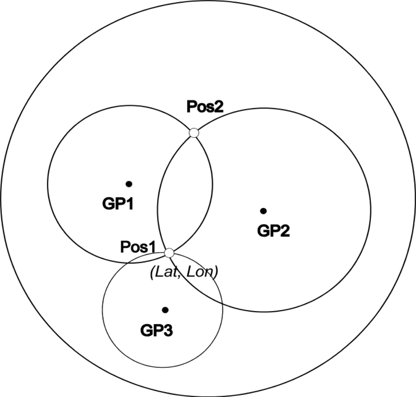
Figure 2. Three circles of equal altitudes for celestial bodies with geographical positions GP1, GP2 and GP3 respectively.
Secondly, we can repeat the method above described for (B1, B3) and (B2, B3). The result will be two additional possible solutions (Lat′, Lon′) and (Lat″, Lon″), normally very close to the first one (Figure 3).
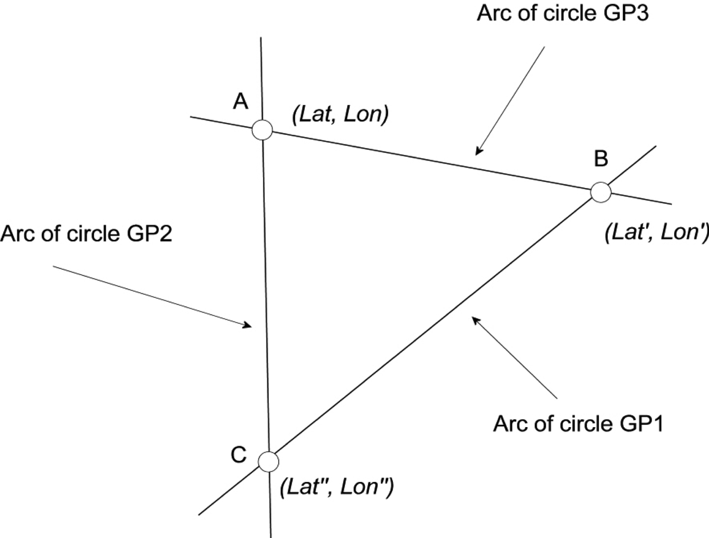
Figure 3. “Uncertainty” triangle ABC after applying the method on the pairs of celestial bodies (B1,B2), (B1,B3) and (B2,B3).
We can consider that the correct position should be inside the “uncertainty” triangle ABC. Since, at this scale, the arcs are reduced to linear segments, we can average latitudes and longitudes to find a more exact solution. Further observations of more stars would give an even more accurate result.
3.2. Testing
Virtual tests were executed. Different points on the globe were selected and their coordinates were marked. Celestial bodies were selected for each location, and their calculated altitudes (Hc) were used as observed altitudes. To find the Hc for the bodies, the US Naval Observatory's Celestial Navigation data at http://aa.usno.navy.mil/data/docs/celnavtable.php was used. The proposed method was then applied, using the related software, and tested to see whether these calculated coordinates coincide with the actual ones. The results are shown in Table 1.
Table 1. Positioning method for the stationary observer. Results of the virtual tests.
The correct solutions are shown in bold. The calculated coordinates show a perfect match with the actual ones. However, in reality, the accuracy of the method mainly depends on the accuracy of the observation (celestial body altitude measurement) as also pointed out by Malkin (Reference Malkin2014).
4. THE MOVING OBSERVER (RUNNING FIX)
To determine the position of a moving observer, the following example will be processed: An observer is at coordinates (Lat1, Lon1) on a vessel moving at constant ground speed V knots with constant course θ (measured eastward from the North, 0° to 360°). At time UTC1 he/she takes the altitude of a celestial body (GHA1, Dec1), H1. At time UTC2, being now at (Lat2, Lon2), he/she takes the altitude of the same, or another, body (GHA2, Dec2), H2. Using Equations (4) and (1):
 $$\sin H1=\sin Lat1\sin Dec1+\cos Lat1\cos Dec1\cos (GHA1+Lon1)$$
 $$\sin H2=\sin Lat2\sin Dec2+\cos Lat2\cos Dec2\cos (GHA2+Lon2)$$
from Equation (18):
 $$Lon2=S\cdot a\cos \left( {\displaystyle{{\sin H2-\sin Lat2\sin Dec2}\over{\cos Lat2\cos Dec2}}} \right)-GHA2$$
S equals −1 if the body is observed east of the observer's meridian, otherwise +1 (see “conventions” in Section 2).
We also have that:
 $$Lat1=Lat2-\Delta Lat$$
with
 $$\Delta Lat=\displaystyle{{V\cos \theta (UTC2-UTC1)}\over{60}}$$
and
 $$Lon1=Lon2-\Delta Lon$$
with
 $$\Delta Lon=\displaystyle{{1}\over{60}}\int\limits_{UTC1}^{UTC2} {\displaystyle{{V\sin \theta \cdot dt}\over{\cos LAT}}}$$
where LAT is the latitude, varying with time, from LAT1 to LAT2.
The integral in Equation (23) can be solved analytically, but, since V and θ are assumed constant, it can be approximated (Daub, Reference Daub1979) with:
 $$\Delta Lon=\displaystyle{{V\sin \theta \lpar {UTC2-UTC1} \rpar }\over{60\cos Lat2}}$$
 If  $\vert {Lat2} \vert <90-\displaystyle{{19}\over{12}}V\lpar {UTC2-UTC1} \rpar $, the approximation's resulting error is less than 0·1'.
Subtracting Equation (17) from Equation (18) and moving to the left side:
 $$\eqalign{\sin Lat1 & \sin Dec1-\sin Lat2\sin Dec2+\cos Lat1\cos Dec1\cos (GHA1+Lon1) \cr &-\cos Lat2\cos Dec2\cos (GHA2+Lon2)-\sin H1+\sin H2=0}$$
Substituting Lon2 from Equation (19), Lat1 from Equations (20) and (21) and Lon1 from Equations (22) and (24), the expression on the left of Equation (25) is a function F only of Lat2, so:
 $$F(Lat2)=0$$
We can find the root numerically, using the secant method iteratively (x = Lat2):
 $$x_n =x_{n-1} -F\lpar {x_{n-1} } \rpar \displaystyle{{x_{n-1} -x_{n-2} }\over{F\lpar {x_{n-1} } \rpar -F\lpar {x_{n-2} } \rpar} }$$
terminating when |x n − x n−1| is less than, say 0·0001°. The longitude Lon2 can then be calculated from Equation (19). The method's algorithm and flowchart is shown in Appendix B.
The secant method requires two initial values, x 0 and x 1, ideally close to the root sought. This does not compromise the independence from an assumed position (just latitude to be exact) because: (a) The secant method is very “tolerant” as far as the initial values are concerned. Choosing initial values “reasonably” far from the actual root does not affect accuracy but only the number of iterations needed. (b) One can find a first initial value without dead reckoning, by using the method described in Section 3, considering the observer as stationary (see Remark 2). A second initial value can be then selected, close to this one.
Also, determining S for Equation (19) does not require an assumed position, since: (a) The navigator most probably has a rough, at least, estimation of the local magnetic declination, hence the local meridian's relative position regarding East and West. (b) Even if this not the case, this can be deduced in various ways (for example, by observing the Sun's meridian passage). (c) If the navigator selects the wrong S, the method will either not converge or it will give an obviously erroneous solution, as in the case of choosing between the two intersection points of two circles of equal altitude. He/she can then repeat the method with the correct S. Nevertheless, the observer must avoid using celestial bodies close to his/her local meridian (meridian angle close to 0°), since this may result to an inaccurate solution or no solution at all, as also mentioned by Kotlaric (Reference Kotlaric1981). For the Sun, this is easily achieved by taking sights when relatively low on the horizon (but at least 10° high, since the variation of refraction due to temperature and atmospheric pressure along the sighting path is less predictable at low altitudes).
4.1. Example (virtual test)
In this example, calculated altitudes (see Section 3.2) are again used instead of observed ones.
On 18 May 2016, a vessel travels with speed 20 kts and course 225°. At UTC1 = 18:00:00 it is at position 45°00′·0N, 45°00′·0W, and the altitude of the Sun (GHA1 = 90°53′·0, Dec1 = 19°45′·5) is H1 = 44°36′·6. At UTC2 = 18:30:00 the Sun is west of the observer's meridian (S = +1) and the corresponding values are GHA2 = 98°23·0, Dec2 = 19°45·8 and H2 = 39°38′·0. Using Equations (19)–(20) and (21)–(23), we estimate that at the time of the second observation, the vessel should be at position 44°52′·9N, 45°10·0W.
(1) Using the “stationary” method we calculate a first assumed latitude of 46°08′·2N.
(2) Using initial values Lat20 = 46 N and Lat21 = 45 N, and S = +1, we apply the secant method described and find the solution: 44°53′·0N, 45°09′·9W, after 3 iterations. The error, compared with the “expected” position, is 0·1 nautical miles.
As with the “stationary” case, we can use more sightings and repeat the procedure to better improve accuracy.
5. CONCLUSIONS
It can be concluded that the method proposed gives satisfactory results, both for the stationary as well as the moving observer, is straightforward, and relatively easy to apply, especially with a programmable calculating device equipped with the appropriate software. The only caveat seems to be that, for the running fix case, celestial bodies relatively far from the observer's local meridian must be selected.
The advantages of the method, apart from independence of GNSS/GPS availability, graphical methods and estimation of an assumed position, and compared with other similar ones are: (a) Relative mathematical simplicity and straight-forwardness, making the solution possible even with a non-programmable calculator. (b) Generality: no need to select particular celestial bodies, for example, each lying in opposite east-west hemispheres relative to the observer's meridian, as other methods require. (c) Use of the formulae from Appendix A, thus eliminating the necessity of the current year's Almanac. (d) Accuracy, practically depending only on the accuracy of the observation. (e) In the case of the running fix problem the use of the secant method and the integration with the “stationary case” eliminates the need of an estimated latitude and significantly reduces the number of iterations required, thus making the solution possible even with a non-programmable calculator. Also, it eliminates the need to derivate function F(Lat2), as the Newton method described by Daub (Reference Daub1979) requires. Both methods always converge, as long as the data entered are correct and the initial value(s) correctly chosen (as mentioned in Section 4, the secant method is also more flexible, concerning the initial values). (f) It is already developed and tested by the author as a working software application, with all the necessary functions and data (see appendices) incorporated and hard-coded.
APPENDIX A – CALCULATION OF CELESTIAL BODIES' APPARENT EQUATORIAL COORDINATES
A1. USEFUL FUNCTIONS
a. Function floor(x), where x a real number. This function is implemented in most programming languages (in some is found as int(x)). It returns the greatest integer smaller than x. For example, floor(3·8) = 3, floor(–2·2) = –3.
b. Function Wrap(x), where x a real number (angle expressed in degrees). This is used to remove the multiples of 360 from an angle. Is defined as:
(A1) $$Wrap(x)=360\left[ {\displaystyle{{x}\over{360}}-\hbox{floor}\left( {\displaystyle{{x}\over{360}}} \right)} \right]$$
c. Function ATAN2(y,x), where x, y real numbers, not both equal to 0. This returns the angle (in radians) between the positive x-axis of a plane and the point given by the coordinates (x, y) on it. In contrast to just computing arctan(y/x), this function gathers information on the signs of the inputs y and x, in order to return the appropriate quadrant of the computed angle, which is not possible for the single-argument arctangent function. It also avoids the problem of division by zero, as atan2(y, 0) will return a valid answer as long as y is non-zero. The function ATAN2 is implemented in most programming languages and is defined as:
(A2)$$\matrix{ {\arctan\left( {\displaystyle{y \over x}} \right)\quad } \hfill & {{\rm if}\;x > 0} \hfill \cr {\arctan \left( {\displaystyle{y \over x}} \right) + \pi \quad } \hfill & {{\rm if}\;x < 0\;{\rm and}\;y \ge 0} \hfill \cr {\arctan \left( {\displaystyle{y \over x}} \right) - \pi \quad } \hfill & {{\rm if}\;x < 0\;{\rm and}\;y < 0} \hfill \cr { + \displaystyle{\pi \over 2}\quad } \hfill & {{\rm if}\;x = 0\;{\rm and}\;y > 0} \hfill \cr { - \displaystyle{\pi \over 2}\quad } \hfill & {{\rm if}\;x = 0\;{\rm and}\;y < 0} \hfill \cr {0\quad } \hfill & {{\rm if}\;x \ne \;0{\rm and }y = 0} \hfill \cr {Undefined\quad } \hfill & {{\rm if}\;x = 0\;{\rm and}\;y = 0} \hfill \cr } $$


A2. COMMON CALCULATIONS
a. Calculate the days and fractions of a day, before or after Jan 1, 2000, 12:00:00 UTC
(A3)where JD is the Julian Date. An equivalent formula is given instead of Equation (A3) (Umland, Reference Umland2011; Albrand and Stein, Reference Albrand and Stein1992) as:$$D=JD+\displaystyle{{UTC}\over{24}}-2451545{\cdot}0$$(A4)where y is the year (4 digits), m is the number of the month, and d the number of the day in the respective month. UTC is the Universal Time in decimal format (e.g., 12 h 30 m 45 s = 12·5125). For May 17, 1999, 12:30:45 UTC, for example, D is −228·978646. The formula is valid from 1 March 1900 to 28 February 2100.$$\eqalign{D = & 367y - {\rm floor}\;\left\{ {1\cdot 75\left[ {y + {\rm floor}\left( {\displaystyle{{m + 9} \over {12}}} \right)} \right]} \right\} + {\rm floor}\;\left( {275\displaystyle{m \over 9}} \right) \cr & + d + \displaystyle{{UTC} \over {24}} - 730531\cdot 5} $$b. Calculate the respective Julian centuries:
(A5)From this point on, the formulae and Table A1 come from Yallop and Hohenkerk (Reference Yallop and Hohenkerk2007), except the Wrap and ATAN2 functions which are not explicitly used in their paper.$$t=\displaystyle{{D}\over{36525}}$$


A3. APPARENT EQUATORIAL COORDINATES OF THE SUN
Convert t to Dynamical Time T:
 $$ \Delta T\lpar t \rpar =0{\cdot}808\lpar {t-2} \rpar ^2\times 10^{-8}$$
 $$ T=t+\Delta T\lpar t \rpar $$
Mean anomaly of the Sun:
 $$G=\hbox{Wrap}\lpar {357^{\circ}{\cdot}529+35999^{\circ}{\cdot}05029T} \rpar $$
Mean ecliptic longitude of the Sun:
 $$L_M =\hbox{Wrap}\lpar {280^{\circ}{\cdot}46645+36000^{\circ}{\cdot}76975T+0^{\circ}{\cdot}0003132T^2} \rpar $$
Mean obliquity of the ecliptic:
 $$\varepsilon _0 =23^{\circ}{\cdot}4393-0^{\circ}{\cdot}01301T-0^{\circ}{\cdot}0000001T^2+0^{\circ}{\cdot}0000006T^3$$
Longitude of Moon's ascending node on the ecliptic:
 $$\Omega =\hbox{Wrap}\lpar {125^{\circ}{\cdot}045-1934^{\circ}{\cdot}136T} \rpar $$
True obliquity of the ecliptic:
 $$ \varepsilon = \varepsilon _0 +0^{\circ}{\cdot}0026\cos \Omega $$
 $$ {GHA}_{Aries} = 100^{\circ}{\cdot}4606+36000^{\circ}{\cdot}76998t+0^{\circ}{\cdot}000387t^2+15UTC-0^{\circ}{\cdot}0048\sin \Omega \cos \varepsilon _0 $$
Important: in the last formula, the time variable is t, not T.
Equation of the centre:
 $$C=\lpar {1^{\circ}{\cdot}9147-0^{\circ}{\cdot}00482T-0^{\circ}{\cdot}000015T^2} \rpar \sin G+0^{\circ}{\cdot}01999\sin 2G$$
Apparent ecliptic longitude of the Sun:
 $$L_T =\hbox{Wrap}\lpar {L_M +C-0^{\circ}{\cdot}0057-0^{\circ}{\cdot}0048\sin \Omega}\rpar $$
Rectangular coordinates:
 $$x=\cos L_T ,y=\cos \varepsilon \sin L_T ,z=\sin \varepsilon \sin L_T$$
Right ascension:
 $$RA=\displaystyle{{180^{\circ}}\over{\pi}}ATAN2\ (y,x)$$
Declination:
 $$Dec=\displaystyle{{180^{\circ}}\over{\pi}}\arcsin \lpar z \rpar $$
GHA:
 $$GHA=\hbox{Wrap}\lpar {GHA_{Aries} -RA} \rpar $$
 $$\hbox{Semidiameter:} \ SD=\displaystyle{{0^{\circ}{\cdot}2666}\over{ {1-0{\cdot}017\cos G}}}=\displaystyle{{1{5}'{\cdot}96}\over{1-0{\cdot}017\cos G}}$$
A4. APPARENT EQUATORIAL COORDINATES OF NAVIGATIONAL STARS
Let λ 0 and β 0 be the ecliptic longitude and latitude, respectively, for epoch and equinox 2000·0, and μ and μ′ their respective centennial rates of change (for values, see Table A1). Note that the time variable is t (see Equation (A5)). Strictly speaking the time variable should be T = t + ΔT(t) (Equations (A6) and (A7)) except when calculating GHA Aries as in Equation (A13). However, since the movement of the stars is very small in the time interval Δ T the change in time scales produces negligible differences (Yallop and Hohenkerk, Reference Yallop and Hohenkerk2007).
a. Calculate the proper motion:
(A21)$$ \lambda _1 =\lambda _0 +\mu t $$(A22)$$ \beta _1 =\beta _0 +{\mu }'t $$b. Apply aberration:
(A23)$$\eqalign{& \lambda _\Theta = 280\cdot 460 + 36000^\circ \cdot 770t \cr & \lambda _2 = \lambda _1 - \displaystyle{{0^\circ \cdot 0057\cos {\rm (}\lambda _1 - \lambda _\Theta {\rm )}} \over {\cos \beta _1}}} $$(A24)$$ \beta _2 =\beta_1 +0^{\circ}{\cdot}0057\sin \lpar {\lambda_1 -\lambda_\Theta } \rpar \sin \beta _1 $$c. Apply precession:
(A25)$$ a=1^{\circ}{\cdot}39697t+0^{\circ}{\cdot}000309t^2 $$(A26)$$ b=0^{\circ}{\cdot}0131t-0^{\circ}{\cdot}00001t^2 $$(A27)$$ c=5^{\circ}{\cdot}1236+0^{\circ}{\cdot}2416t $$(A28)$$ \beta _3 =\beta _2 +b\sin \lpar {\lambda_2 +c} \rpar $$(A29)Apply nutation:$$ \lambda _3 =\lambda _2 +a-b\cos \lpar {\lambda_2 +c} \rpar \tan \beta _3 $$(A30)$$ \lambda =\lambda _3 -0^{\circ}{\cdot}0048\sin \Omega $$(A31)$$ \beta =\beta _3 $$d. Finally:


Rectangular coordinates:
 $$ x=\cos \beta \cos \lambda $$
 $$ y=\cos \varepsilon \cos \beta \sin \lambda -\sin \varepsilon \sin \beta $$
 $$ z=\sin \varepsilon \cos \beta \sin \lambda +\cos \varepsilon \sin \beta $$
Right ascension:
 $$RA=\displaystyle{{180^{\circ}}\over{\pi}}\hbox{ATAN2}(y,x)$$
Declination:
 $$Dec=\displaystyle{{180^{\circ}}\over{\pi}}\arcsin \lpar z \rpar $$
 $$ {GHA}_{Aries} = 100^{\circ}{\cdot}4606+36000^{\circ}{\cdot}77005t+0^{\circ}{\cdot}000388t^2+15UTC-0^{\circ}{\cdot}0048\sin \Omega \cos \varepsilon$$
GHA:
 $$GHA=\hbox{Wrap}\lpar {GHA_{Aries} -RA} \rpar $$
Table A1. Longitude and Latitude referred to the ecliptic and mean equinox of J2000·0

APPENDIX B

APPENDIX C. SEXTANT ALTITUDE CORRECTIONS
Altitude corrections are necessary to eliminate systematic altitude errors and to reduce the altitude measured relative to the visible horizon, to the altitude with respect to the celestial horizon and the centre of the Earth (Umland, Reference Umland2011).
In the following formulae, the altitudes are measured in degrees and minutes of arc, while the corrections in minutes of arc. Let H s the altitude initially measured with the sextant.
C1. INDEX ERROR (IE)
The index error is inherent to the particular sextant used and must be known. It can be either positive, if the displayed value is greater than the actual one, or negative in the opposite case. So:
 $$1^{\rm st}\ correction{:} \quad H_1 = H_s - IE $$
If using an artificial horizon (not bubble sextant), H 1 (not H s) must be divided by 2.
C2. DIP OF HORIZON (D)
This is due to the curvature of the Earth's surface. It is the angle between the line perpendicular to the observer at the height of the eye and the visible horizon.
 $$D=1{\cdot}76\sqrt{HE}\ ({HE}\ \hbox{in metres})\ \hbox{or}\ D=0{\cdot}97\sqrt{HE}\ ({HE}\ \hbox{in}\ \hbox{feet})$$
Where HE is the height of eye of the observer.
 $$2^{\rm nd}\;{\rm correction}{:} \;\;\;H_2 = H_1 - D$$
Notice: This correction must be omitted if any kind of artificial horizon is used, including a bubble sextant.
C3. CORRECTION FOR ATMOSPHERIC REFRACTION (R)
For altitudes between 15° and 90°:
 $$R=\displaystyle{{1{\cdot}0067}\over{\tan H_2 }}$$
For altitudes between 0° and 15°:
 $$R=\displaystyle{{34{\cdot}133+4{\cdot}197H_2 +0{\cdot}00428H_2^2 }\over{1+0{\cdot}505H_2 +0{\cdot}0845H_2^2}}$$
Refraction is influenced by temperature and atmospheric pressure. The formulae above are valid for temperature 10°C and pressure 1010 mbar. For other values of temperature and pressure, R must be multiplied by a factor f:
 $$\eqalign{& f = 0\cdot 2802\displaystyle{P \over {273 + T}}\;(P\;{\rm in}\;{\rm mbar},T\;{\rm in}\;^\circ C)\;{\rm or} \cr & f = 17\cdot 0969\displaystyle{P \over {460 + T}}\;(P\,{\rm in}\;{\rm in}{\rm .Hg,}\;T\;{\rm in}\;^\circ F)} $$
 $$ 3^{\rm rd} \hbox{correction: } H_3 =H_2 -fR $$
C4. SUN'S SEMIDIAMETER
If the observed body is the Sun, it's Semidiameter (SD – see Appendix A, Equation (A20)) must be taken into account, because usually the lower or the upper limb is observed. If a bubble sextant is used (which is less accurate), we usually observe the centre of the body, so this correction is omitted.
 $$\eqalign{& 4^{{\rm th}}{\rm correction}:\quad H_4 = H_3 \pm SD \cr & ( + \;{\rm for\;the\;lower\;limb},\; - {\rm for\;the\;upper\;limb})} $$
The altitude obtained after applying the above corrections, is the observed altitude:
 $$ H_o = H_4 $$


