2. Atmospheric refraction model analysis for aircraft

According to the law of refraction, starlight will be refracted and bent inward to the geocentre when passing through the atmosphere. Therefore the apparent position of a star will be a little higher than its actual one. For the certain position of a UAV, the unit vectors of the stellar apparent direction u_a and the real direction u_r (reverse direction of starlight) in geocentric equatorial inertial coordinate system (denoted as frame i), together with the zenith direction ζ are coplanar, which is defined as the stellar azimuth plane μ_a. The angle between u_a and u_r is defined as the starlight refraction angle ρ, whose relationship with stellar apparent zenith distance z_a and real zenith distance z_r is shown in Figure 1, where R_e is the radius of the Earth; h is the altitude of the vehicle; μ_h is the local horizon plane, μ_h⊥μ_a; u_s and u_m are unit directional vectors of the sun and the moon, with the exclusion angles ε_s and ε_m.

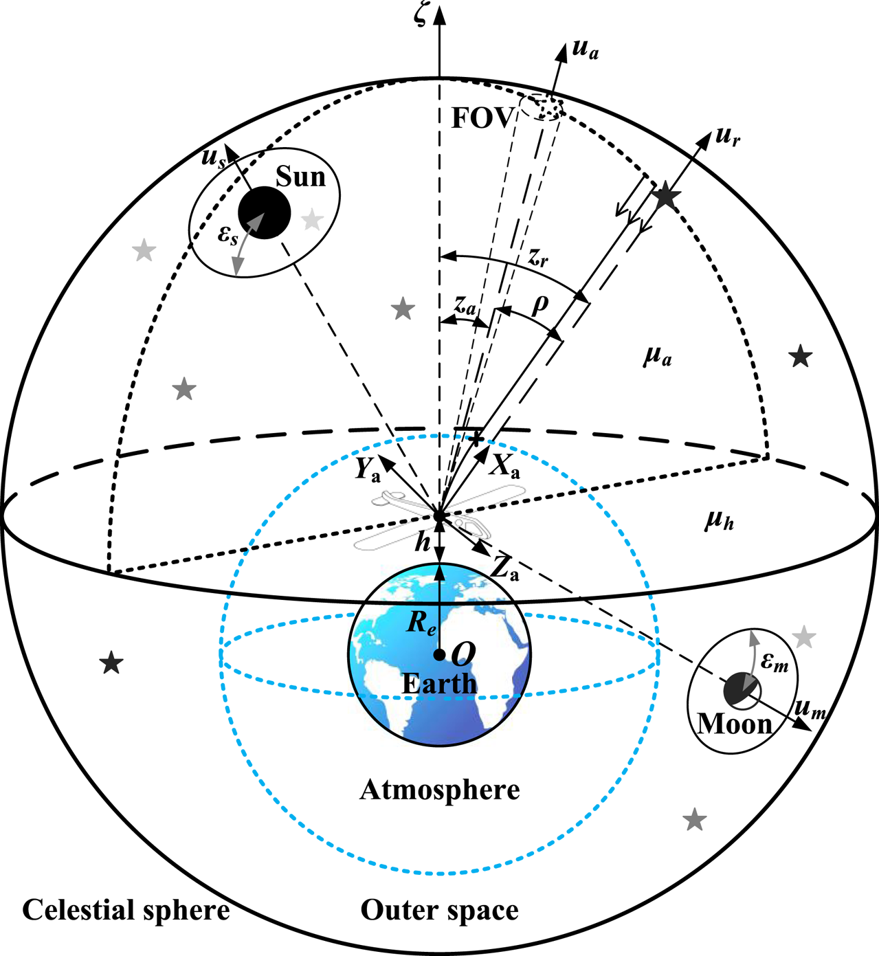
Figure 1. Geometric description of atmospheric refraction (variable scale)

In the body coordinate system (denoted as frame b), the UAV's longitudinal axis is defined as the Y _b axis. The Z _b axis is upward in the longitudinal plane. The coordinate conversion matrix $\boldsymbol{C}_{\rm i}^{\rm b}$ from frame i to frame b can be calculated by the attitude determination method, with the right ascension α, declination δ and roll angle γ of the Z _b axis direction obtained from the corresponding three Euler angles: 90° + α, 90° − δ and γ in a rotation order of 3-1-3. α, δ and γ are assigned as the absolute attitude angles of the aircraft.

The apparent stellar direction and real stellar direction in frame b are assigned as v_a and v_r. v_a can be measured by star sensor in the star sensor coordinate system (denoted as frame s) and then transferred to frame b by the installed matrix $\boldsymbol{M}_{\rm b}^{\rm s}$. When the identified star is given and the attitude is determined, v_r can be obtained through u_r and $\boldsymbol{C}_{\rm i}^{\rm b}$. Thus,

(1)\begin{equation}\rho = {\rm arccos}({\boldsymbol{u}_{\boldsymbol{a}}^{\rm T}{\boldsymbol{u}_{\boldsymbol{r}}}} )= {\rm arccos}({\boldsymbol{v}_{\boldsymbol{a}}^{\rm T}{\boldsymbol{v}_{\boldsymbol{r}}}} )= {\rm arccos}({\boldsymbol{v}_{\boldsymbol{a}}^{\rm T}\boldsymbol{C}_{\rm i}^{\rm b}{\boldsymbol{u}_{\boldsymbol{r}}}} )\end{equation}

In practical application, z_a can be calculated through refraction tables or empirical formulae based on the refraction angle and the ambient condition of the vehicle. In this paper, the empirical formula provided by the Chinese Astronomical Almanac (The Purple Mountain Observatory, 2021) is chosen to analyse the problem as follows:

(2)\begin{align}{\rho _0} & = \frac{\rho }{{1 + {\alpha _A}{M_A} + {N_A}}}\end{align}

(3)\begin{align}{M_A} & = \frac{{ - 0{\cdot} 00383{T_c}}}{{1 + 0{\cdot} 00367{T_c}}}\end{align}

(4)\begin{align}{N_A} & = \frac{P}{{133{\cdot} 322 \times 760}} - 1\end{align}

(5)\begin{align}P & = P^{\prime}[{1 - 0{\cdot} 00264\cos 2\varphi - 0{\cdot} 000163({{{T^{\prime}}_c} - {T_c}} )} ]\end{align}

(6)\begin{align}{z_a} & = \arctan \frac{{{\rho _0}}}{{60{\cdot} 2^{\prime\prime} }}\end{align}

where ρ ₀ is the mean atmospheric refractivity; M_A, N_A and α_A (α_A = 1 generally; when z_a is large, α_A will be adjusted) are modified parameters; T_c is ambient centigrade temperature; P is ambient barometric pressure in units of Pa; T_c′ is measuring centigrade temperature of mercury in the barometer; P′ is measuring barometric pressure in units of Pa. Ambient barometric pressure and thermodynamic temperature T of a standard day are described by the ISA (Kurzke and Halliwell, Reference Kurzke and Halliwell2018). In the range of aircraft actual flight altitude, P and T satisfy

(7)\begin{align}P & = \begin{cases} 101,325 \times {{\left( {{\rm 1} - 0{\cdot} 0225577 \times \dfrac{h}{{1000}}} \right)}^{5{\cdot} 25588}}{\rm Pa }, & {h < 11,000\,{\rm m}}\\ {22,632 \times {e^{\tfrac{{11000 - h}}{{6341{\cdot} 62}}}}{\rm Pa },}& {11,000\,{\rm m} \le h \le 25,000\,{\rm m}} \end{cases}\end{align}

(8)\begin{align}T & = \begin{cases} {288{\cdot} 15\,{\rm K} - 6{\cdot} 5 \times \dfrac{h}{{1000}},}& {h < 11,000\,{\rm m}}\\ {216{\cdot} 65\,{\rm K ,}}& {11,000\,{\rm m} \le h \le 25,000\,{\rm m}} \end{cases}\end{align}

Therefore,

(9)\begin{equation}{z_r} = {z_a} + \rho \end{equation}

The empirical formulae of Equations (2) to (9) have directly established the functional relation among z_r, z_a and ρ. For this, Ning and Wang (Reference Ning and Wang2013) demonstrated that the zenith error Δζ increases with increasing celestial altitude (i.e., 90°−z_r) by curve-fitting method simulation. The next step is to analyse its spherical geometry.

When u_r is identified, through the atmospheric refraction model, the estimated zenith direction $\hat{\boldsymbol{\zeta }}$ is determined by the estimated stellar apparent direction ${\hat{\boldsymbol{u}}_{\boldsymbol{a}}}$ with the error Δu_a which is affected by attitude accuracy, as shown in Figure 2.

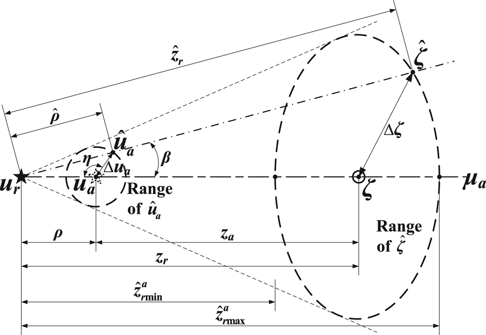
Figure 2. Geometric relationship of error ranges projected onto the celestial sphere

The spherical triangles satisfy

(10)\begin{align}\cos \hat{\rho } & = \cos \rho \cos \Delta {u_a} + \sin \rho \sin \Delta {u_a}\cos \eta \end{align}

(11)\begin{align}\frac{{\sin \beta }}{{\sin \Delta {u_a}}} & = \frac{{\sin \eta }}{{\sin \hat{\rho }}}\end{align}

(12)\begin{align}\cos \Delta \zeta & = \cos {\hat{z}_r}\cos {z_r} + \sin {\hat{z}_r}\sin {z_r}\cos \beta \end{align}

where

(13)\begin{equation}{\hat{z}_r} = \hat{\rho } + {\rm arctan}\frac{{\hat{\rho }}}{{60{\cdot} 2\mathrm{^{\prime\prime} }({1 + {M_A} + {N_A}} )}}\end{equation}

Particularly in μ_a direction, the estimated real zenith distance $\hat{z}_r^a$ satisfies

(14)\begin{equation} \begin{cases} \hat{z}_{r\min }^a = \rho - \Delta {u_a} + \arctan \dfrac{{\rho - \Delta {u_a}}}{{60{\cdot} 2\mathrm{^{\prime\prime} }({1 + {M_A} + {N_A}} )}}\quad (\eta = \beta = 0)\\ \hat{z}_{r\max }^a = \rho + \Delta {u_a} + \arctan \dfrac{{\rho + \Delta {u_a}}}{{60{\cdot} 2\mathrm{^{\prime\prime} }({1 + {M_A} + {N_A}} )}}\quad (\eta = 180^\circ ,\beta = 0) \end{cases}\end{equation}

Thus

(15)\begin{align}\Delta \hat{z}_r^a = \hat{z}_{r\;{\rm max}}^a - \hat{z}_{r\;{\rm min}}^a = 2\Delta {u_a} + \arctan \frac{{\rho + \Delta {u_a}}}{{60{\cdot} 2\mathrm{^{\prime\prime} }({1 + {M_A} + {N_A}} )}} - \arctan \frac{{\rho - \Delta {u_a}}}{{60{\cdot} 2\mathrm{^{\prime\prime} }({1 + {M_A} + {N_A}} )}}\end{align}

(16)\begin{align}\frac{{{\rm d}\Delta \hat{z}_r^a}}{{{\rm d}\rho }} = \frac{{60{\cdot} 2^{\prime\prime} ({1 + {M_A} + {N_A}} )}}{{{{({60{\cdot} 2\mathrm{^{\prime\prime} }({1 + {M_A} + {N_A}} )} )}^2} + {{({\rho + \Delta {u_a}} )}^2}}} - \frac{{60{\cdot} 2\mathrm{^{\prime\prime} }({1 + {M_A} + {N_A}} )}}{{{{({60{\cdot} 2^{\prime\prime} ({1 + {M_A} + {N_A}} )} )}^2} + {{({\rho - \Delta {u_a}} )}^2}}} < 0\end{align}

This indicates that the zenith error range shrinks with increasing ρ (equivalent to z_a or z_r). The whole result will be given in Section 5.1.

For the purpose of calculating the zenith direction, the stellar azimuth coordinate system (denoted as frame a) is established, with the X _a axis oriented to the stellar real direction and Y _a axis upward in plane μ_a, as shown in Figure 1. Obviously,

(17)\begin{equation}{\boldsymbol{\zeta }_{\rm a}} = {\left[ {\begin{array}{*{20}{c}} {\cos {z_r}}& {\sin {z_r}}& 0 \end{array}} \right]^{\rm T}}\end{equation}

The vector-matrices V and W are established as

(18)\begin{align}\boldsymbol{V} & = \left[ {\begin{matrix} {{\boldsymbol{V}_1}}& {{\boldsymbol{V}_2}}& {{\boldsymbol{V}_3}} \end{matrix}} \right]\quad {\boldsymbol{V}_1} = {\boldsymbol{v}_{\boldsymbol{r}}}\quad {\boldsymbol{V}_2} = {\boldsymbol{v}_{\boldsymbol{a}}}\quad {\boldsymbol{V}_3} = \frac{{{\boldsymbol{v}_{\boldsymbol{r}}} \times {\boldsymbol{v}_{\boldsymbol{a}}}}}{{|{{\boldsymbol{v}_{\boldsymbol{r}}} \times {\boldsymbol{v}_{\boldsymbol{a}}}} |}} \end{align}

(19)\begin{align}\boldsymbol{W} & = \left[ {\begin{matrix} {{\boldsymbol{W}_1}}& {{\boldsymbol{W}_2}}& {{\boldsymbol{W}_3}} \end{matrix}} \right]\quad {\boldsymbol{W}_1} = {\boldsymbol{X}_{\rm a}} = \left[ {\begin{array}{*{20}{c}} 1\\ 0\\ 0 \end{array}} \right] \quad {\boldsymbol{W}_2} = \left[ {\begin{array}{*{20}{c}} {\cos \rho }\\ {\sin \rho }\\ 0 \end{array}} \right]\quad {\boldsymbol{W}_3} = {\boldsymbol{Z}_{\rm a}} = \left[ {\begin{array}{*{20}{c}} 0\\ 0\\ 1 \end{array}} \right]\end{align}

Hence, the orthogonalised coordinate conversion matrix $\boldsymbol{C}_{\rm a}^{\rm b}$ is

(20)\begin{align}\boldsymbol{C}_{\rm a}^{\rm b} & = \frac{1}{2}({3\boldsymbol{I} - \boldsymbol{C}_0^{\rm T}{\boldsymbol{C}_0}} )\boldsymbol{C}_0^{\rm T}\end{align}

(21)\begin{align}{\boldsymbol{C}_0} & = \boldsymbol{W}{\boldsymbol{V}^{\rm T}}{({\boldsymbol{V}{\boldsymbol{V}^{\rm T}}} )^{ - 1}}\end{align}

where C₀ is the non-orthogonal matrix.

λ_b and φ_b are the longitude and latitude coordinates of zenith direction in frame b, which satisfy

(22)\begin{equation}{\boldsymbol{\zeta }_{\rm b}} = {\left[ {\begin{matrix} {\cos {\varphi_b}\cos {\lambda_b}}& {\cos {\varphi_b}\sin {\lambda_b}}& {\sin {\varphi_b}} \end{matrix}} \right]^{\rm T}} = \boldsymbol{C}_{\rm a}^{\rm b}{\boldsymbol{\zeta }_{\rm a}}\end{equation}

Through calculating the real-time Greenwich hour angle of Aries A _ϒ, the conversion matrix $\boldsymbol{C}_{\rm i}^{\rm e}$ from frame i to geocentric equatorial rotating coordinate system (denoted as frame e) can be obtained. Therefore, the geographical longitude λ and latitude φ can be solved by

(23)\begin{equation}{\left[ {\begin{matrix} {\cos \varphi \cos \lambda }& {\cos \varphi \sin \lambda }& {\sin \varphi } \end{matrix}} \right]^{\rm T}} = \boldsymbol{C}_{\rm i}^{\rm e}\boldsymbol{C}_{\rm b}^{\rm i}{\boldsymbol{\zeta }_{\rm b}}\end{equation}

Assigning the east-north-zenith (E-N-U) coordinate system (denoted as frame n) as the navigation coordinate system, the conversion matrix $\boldsymbol{C}_{\rm n}^{\rm e}$ can be calculated through the two Euler angles −(90° − φ) and −(90° + λ) in a rotation order of 1-3. Thus the conversion matrix $\boldsymbol{C}_{\rm n}^{\rm b}$ can be deduced by $\boldsymbol{C}_{\rm i}^{\rm b}$, $\boldsymbol{C}_{\rm i}^{\rm e}$ and $\boldsymbol{C}_{\rm n}^{\rm e}$, with three Euler angles named respectively as yaw angle -ψ, pitch angle θ and roll angle ϕ in a rotation order of 3-1-2. ψ, θ and ϕ are assigned as the relative attitude angles of the aircraft.

The analysis above presents the relation between the position and attitude parameters of the UAV. However, neither the precise attitude nor position information can be directly measured by CNS alone in refractive conditions. High accuracy attitude and position determinations are key problems. In Sections 3 and 4, these will be further discussed.

3. Research on triple-FOV star sensors navigation by stellar refraction

Generally, for spacecraft, if the observed stars are successfully identified by image matching algorithm, then attitude with high accuracy can be ensured by high-precision star sensor and optimised attitude determination method. However, for aircraft, the atmosphere will absorb, scatter and refract the starlight. This may seriously decrease the light intensity and increase background noise, making starlight harder to detect, especially in daytime. As a result, both the star pattern recognition and attitude determination accuracy will be affected.

To solve these problems, the narrow FOV star sensor has been developed to improve the sensitivity of CCD (Charge Coupled Device) arrays by sacrificing the detection range. Thus, the application of multiple-FOV star sensors is necessary to ensure both the observability and the precision (Wu et al., Reference Wu, Wang and Wang2015, Reference Wu, Xu, Wang, Lyu and Li2019). On this basis, we can extract the refractive images from combined star map and increase the matching tolerance to maintain the recognition rate. This can be much easier or even unnecessary when sensors are working in tracking mode (Li et al., Reference Li, Sun and Zhang2015; Wang et al., Reference Wang, Zhu, Qin, Zhang and Li2017a).

The identified stars in combined FOV are shown in Figure 3, where S_j (j = 1, 2, 3) are boresight projections on the celestial sphere corresponding to star sensor I, II or III. For each observed star, the projections of u_al, u_rl and ζ are on the arc where the celestial sphere meets with μ_al (l = 1, 2, 3…).

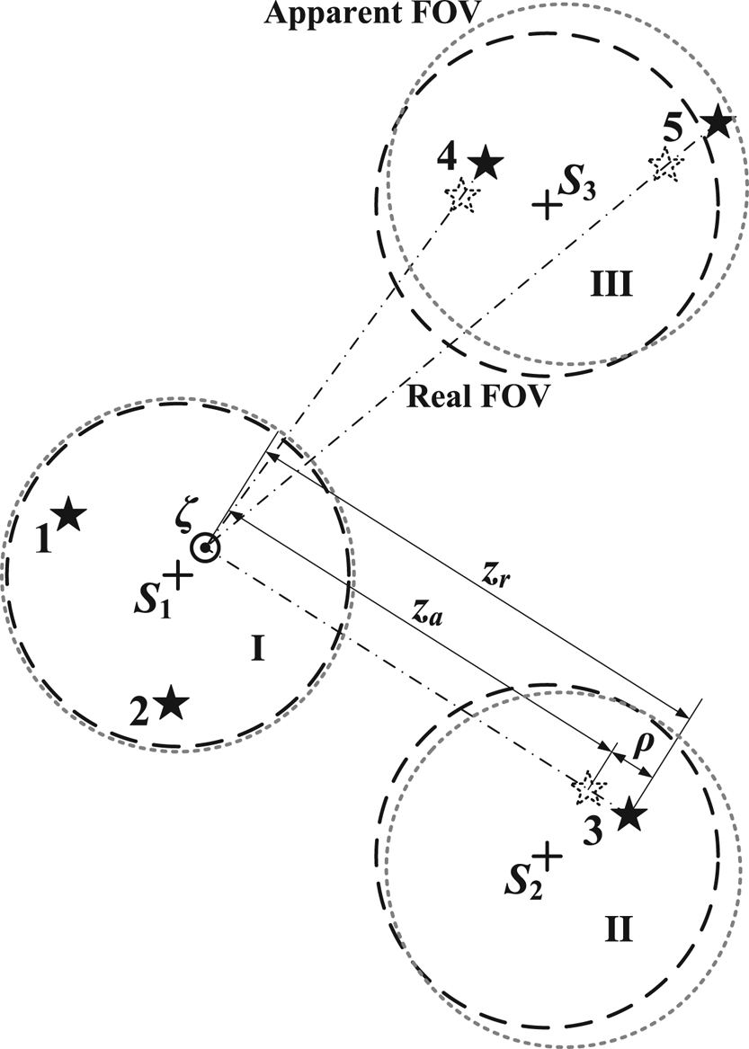
Figure 3. Geometric relationship of multiple FOVs and stars projected onto the celestial sphere

Obviously, ζ is the common intersecting line of all the stellar azimuth planes. When the precise ζ is calculated, the position can be acquired. However, according to Section 2, calculations of the zenith direction and attitude are coupled. So the following two schemes are designed to seek the efficient method.

3.1 Coplanar distribution scheme

When a UAV is cruising straight and level, the Z _b axis can be considered as orienting to the zenith. That means that, if the observed starlight orientation is close to the Z _b axis (Star 1 and 2 in Sensor I), then ρ will be very small, i.e.,

(24)\begin{equation}\begin{cases} {{\boldsymbol{u}_{\boldsymbol{a}l}} \approx {\boldsymbol{u}_{\boldsymbol{r}l}}}\\ {{\boldsymbol{v}_{\boldsymbol{a}l}} \approx {\boldsymbol{v}_{\boldsymbol{r}l}}} \end{cases} (l = 1,2)\end{equation}

Therefore the absolute attitude of the vehicle can be directly determined by at least two identified stars in theory (Shuster and Oh, Reference Shuster and Oh1981; Zhu et al., Reference Zhu, Ma, Cheng and Zhou2017). Based on this, a coplanar distribution scheme by three star sensors is designed to analyse the problem, as shown in Figure 4, where α_s (0 ≤ α_s ≤ 90°) is marked as the strapdown installation angle.

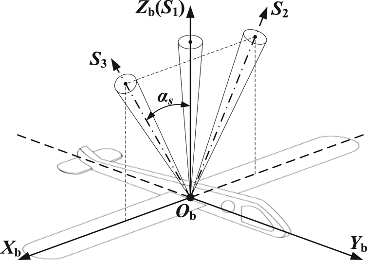
Figure 4. Installation of the coplanar distribution scheme

Sensor I is used to measure the ‘non-refracted’ stars and estimate the attitude, whereas Sensors II and III, in a symmetrical distribution, are utilised to observe the refracted stars and calculate the geographical coordinates by the atmospheric refraction model with $\hat{\boldsymbol{C}}_{\rm i}^{\rm b}$ provided by Sensor I. Furthermore, sensors on both sides can increase the observation scope and ensure the FOVs do not scan blind areas (e.g. the sun and the moon) simultaneously. The flowchart is presented in Figure 5.

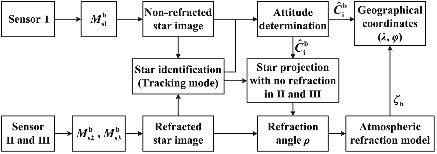
Figure 5. Flowchart of the coplanar distribution scheme

However, this scheme has two disadvantages. First, limited by the FOV of Sensor I, the detection probability is low and the angular distance between different starlight vectors is rather small, which may lead to big errors in attitude. Second, when the aircraft manoeuvres in flight, boresight of Sensor I will deviate from the zenith direction and refraction cannot be ignored. Therefore, general cases should be studied.

3.2 Triangular distribution scheme

The universality of triple-FOV star sensors in triangular distribution can enhance the practicability of CNS. These are installed, as shown in Figure 6, to satisfy the omnibearing observation.

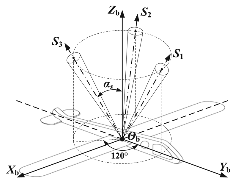
Figure 6. Installation of the triangular distribution scheme

Through derivation of the Jacobi identity (see Appendix part in details),

(25)\begin{equation}{({{\boldsymbol{v}_{\boldsymbol{a}}} \times {\boldsymbol{v}_{\boldsymbol{r}}}{\cdot} {\boldsymbol{\zeta }_{\rm b}}} )^2} = 1 - {({{\boldsymbol{v}_{\boldsymbol{a}}}{\cdot} {\boldsymbol{v}_{\boldsymbol{r}}}} )^2} - {({{\boldsymbol{v}_{\boldsymbol{r}}}{\cdot} {\boldsymbol{\zeta }_{\rm b}}} )^2} - {({{\boldsymbol{\zeta }_{\rm b}}{\cdot} {\boldsymbol{v}_{\boldsymbol{a}}}} )^2} + 2({{\boldsymbol{v}_{\boldsymbol{a}}}{\cdot} {\boldsymbol{v}_{\boldsymbol{r}}}} )({{\boldsymbol{v}_{\boldsymbol{r}}}{\cdot} {\boldsymbol{\zeta }_{\rm b}}} )({{\boldsymbol{\zeta }_{\rm b}}{\cdot} {\boldsymbol{v}_{\boldsymbol{a}}}} )= 0\end{equation}

Based on this, the loss function (Wang et al., Reference Wang, Gao and Wang2021a) is established as

(26)\begin{align} F({\boldsymbol{C}_{\rm i}^{\rm b},{\boldsymbol{\zeta }_{\rm b}}} )& =\sum_{l = 1}^n {{a_l}{{({{\boldsymbol{v}_{\boldsymbol{a}l}} \times {\boldsymbol{v}_{\boldsymbol{r}l}}{\cdot} {\boldsymbol{\zeta }_{\rm b}}} )}^2}} \notag\\ & =\sum_{l = 1}^n {{a_l}({1 - {{({\boldsymbol{v}_{\boldsymbol{a}l}^{\rm T}\boldsymbol{C}_{\rm i}^{\rm b}{\boldsymbol{u}_{\boldsymbol{r}l}}} )}^2} - {{({\boldsymbol{\zeta }_{\rm b}^{\rm T}\boldsymbol{C}_{\rm i}^{\rm b}{\boldsymbol{u}_{\boldsymbol{r}l}}} )}^2} - {{({\boldsymbol{\zeta }_{\rm b}^{\rm T}{\boldsymbol{v}_{\boldsymbol{a}l}}} )}^2} + 2({\boldsymbol{v}_{\boldsymbol{a}l}^{\rm T}\boldsymbol{C}_{\rm i}^{\rm b}{\boldsymbol{u}_{\boldsymbol{r}l}}} )({\boldsymbol{\zeta }_{\rm b}^{\rm T}\boldsymbol{C}_{\rm i}^{\rm b}{\boldsymbol{u}_{\boldsymbol{r}l}}} )({\boldsymbol{\zeta }_{\rm b}^{\rm T}{\boldsymbol{v}_{\boldsymbol{a}l}}} )} )} \end{align}

where n is the total number of observed stars, a_l (l = 1,…,n) are a set of nonnegative weights satisfying

(27)\begin{equation}\sum_{l = 1}^n {{a_l}} = 1\end{equation}

Obviously, the less estimated errors of $\hat{\boldsymbol{C}}_{\rm i}^{\rm b}$ and ${\hat{\boldsymbol{\zeta }}_{\rm b}}$ are, the smaller function value is. Combined with Equation (22), variables of the loss function are converted into two scalars (λ_b and φ_b) and one matrix, which cannot be solved by existing classical methods on account of strong nonlinearity. Now we try to establish a conjugate gradient iterative algorithm to testify the improvement of navigation accuracy by reducing the loss function value.

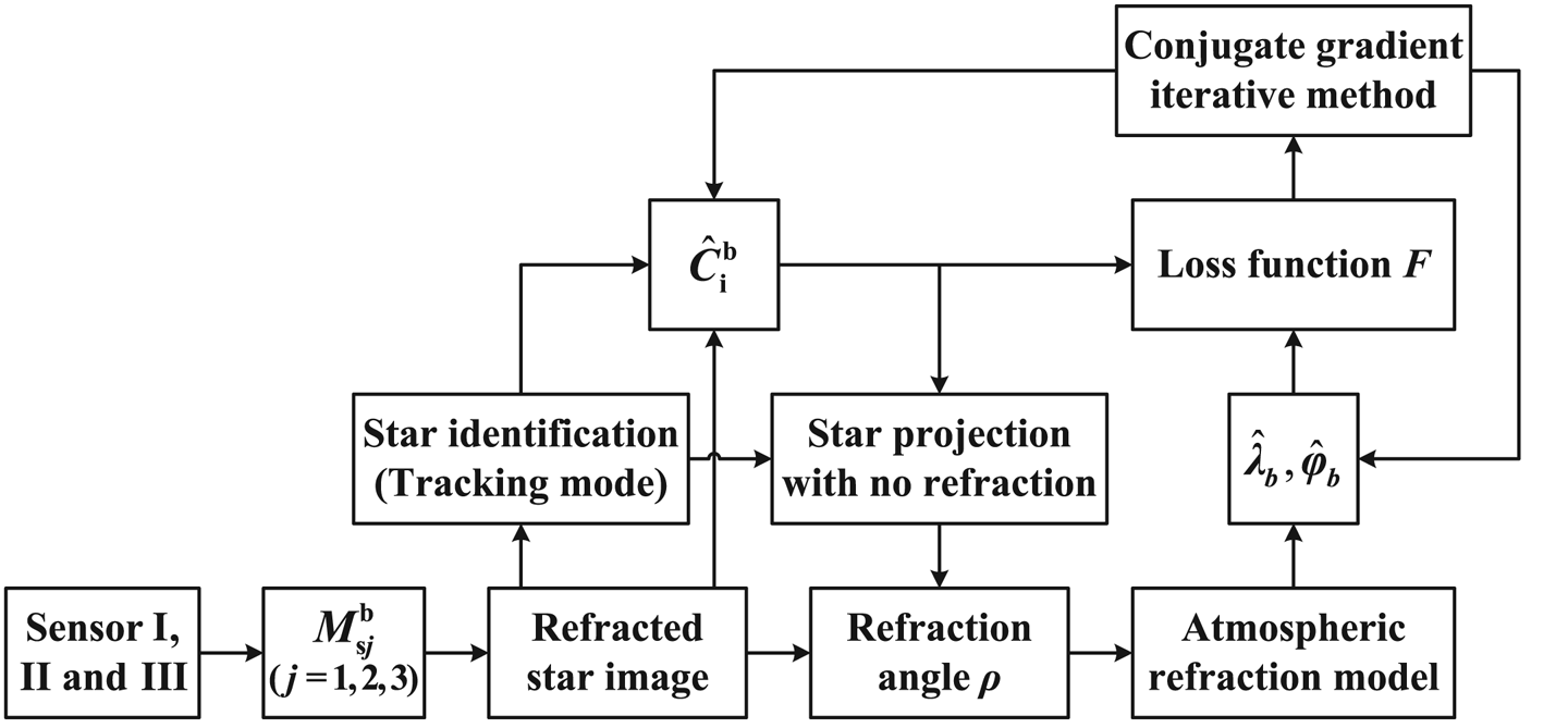
Actual observed stars are measured in the combined FOV of I, II and III, so a rough attitude $\hat{\boldsymbol{C}}_{\rm i}^{\rm b}$ can be estimated without refraction compensation, thereby obtaining ${\hat{\lambda }_b}$ and ${\hat{\varphi }_b}$ in a similar way. Regarding $\hat{\boldsymbol{C}}_{\rm i}^{\rm b}$ as a constant matrix in each iteration, the loss function can be processed by conjugate gradient iterative method to update attitude and position information, as shown in Figure 7 (Rivaie et al., Reference Rivaie, Mamat and Abashar2015; Liu et al., Reference Liu, Feng and Zou2018).

Figure 7. Flowchart of the triangular distribution scheme

The gradient function satisfies

(28)\begin{align}\boldsymbol{g} &= {\left[ {\begin{array}{*{20}{c}} {\dfrac{{\partial F}}{{\partial {\lambda_b}}}}& {\dfrac{{\partial F}}{{\partial {\varphi_b}}}} \end{array}} \right]^{\rm T}}\end{align}

(29)\begin{align}\frac{{\partial F}}{{\partial {\lambda _b}}} &= \frac{{\partial \boldsymbol{\zeta }_{\rm b}^{\rm T}}}{{\partial {\lambda _b}}}{\cdot} \frac{{\partial F}}{{\partial {\boldsymbol{\zeta }_{\rm b}}}} = \left[ {\begin{matrix} {-} \cos {{\hat{\varphi }}_b}\sin {{\hat{\lambda }}_b} & {\cos {{\hat{\varphi }}_b}\cos {{\hat{\lambda }}_b}}& 0 \end{matrix}} \right]{\cdot} \frac{{\partial F}}{{\partial {\boldsymbol{\zeta }_{\rm b}}}}\end{align}

(30)\begin{align}\frac{{\partial F}}{{\partial {\varphi _b}}} &= \frac{{\partial \boldsymbol{\zeta }_{\rm b}^{\rm T}}}{{\partial {\varphi _b}}}{\cdot} \frac{{\partial F}}{{\partial {\boldsymbol{\zeta }_{\rm b}}}} = {\left[ {\begin{matrix} { {-} \sin {{\hat{\varphi }}_b}\cos {{\hat{\lambda }}_b}}& { {-} \sin {{\hat{\varphi }}_b}\sin {{\hat{\lambda }}_b}}& {\cos {{\hat{\varphi }}_b}} \end{matrix}} \right]^{\rm T}}{\cdot} \frac{{\partial F}}{{\partial {\boldsymbol{\zeta }_{\rm b}}}}\end{align}

(31)\begin{align}\frac{{\partial F}}{{\partial {\boldsymbol{\zeta }_{\rm b}}}} &= ({ - 2} )\cdot \left[ {\sum_{l = 1}^n {{a_l}{\boldsymbol{v}_{\boldsymbol{a}l}}\boldsymbol{v}_{\boldsymbol{a}l}^{\rm T}} + \hat{\boldsymbol{C}}_{\rm i}^{\rm b}\left( {\sum_{l = 1}^n {{a_l}{\boldsymbol{u}_{\boldsymbol{r}l}}\boldsymbol{u}_{\boldsymbol{r}l}^{\rm T}} } \right)\hat{\boldsymbol{C}}_{\rm b}^{\rm i} - \sum_{l = 1}^n {{a_l}\boldsymbol{v}_{\boldsymbol{a}l}^{\rm T}\hat{\boldsymbol{C}}_{\rm i}^{\rm b}{\boldsymbol{u}_{\boldsymbol{r}l}}({{\boldsymbol{v}_{\boldsymbol{a}l}}{{({\hat{\boldsymbol{C}}_{\rm i}^{\rm b}{\boldsymbol{u}_{\boldsymbol{r}l}}} )}^{\rm T}} + \hat{\boldsymbol{C}}_{\rm i}^{\rm b}{\boldsymbol{u}_{\boldsymbol{r}l}}\boldsymbol{v}_{\boldsymbol{a}l}^{\rm T}} )} } \right]{\cdot} {\hat{\boldsymbol{\zeta }}_{\rm b}}\end{align}

Therefore, the conjugate gradient iterative method contains the following steps:

Step 1: When ‖g_k‖ ≤ ε (k = 0, 1, 2…, ε is the specified precision), iteration algorithm stops.

Step 2: Determine the iteration step length α_k by Armijo line search method (Nocedal and Wright, Reference Nocedal and Wright2006). Then,

(32)\begin{equation}{\left[ {\begin{array}{*{20}{c}} {{{\hat{\lambda }}_b}}\\ {{{\hat{\varphi }}_b}} \end{array}} \right]_{k + 1}} = {\left[ {\begin{array}{*{20}{c}} {{{\hat{\lambda }}_b}}\\ {{{\hat{\varphi }}_b}} \end{array}} \right]_k}\boldsymbol{+ }{\alpha _k}{\boldsymbol{d}_k}\end{equation}

where the initial search direction d₀ = −g₀.

Step 3: Revise the refracted starlight by ${({\hat{\lambda }_b},{\hat{\varphi }_b})_{k + 1}}$ through atmospheric refraction model and update the attitude $\hat{\boldsymbol{C}}_{\rm i}^{\rm b}$.

Step 4: Compute F_k + 1 and g_k + 1 by $\hat{\boldsymbol{C}}_{\rm i}^{\rm b}$ and ${({\hat{\lambda }_b},{\hat{\varphi }_b})_{k + 1}}$.

Step 5: Compute β_k + 1 by

(33)\begin{equation}{\beta _{k + 1}} = \frac{{\boldsymbol{g}_{k + 1}^{\rm T}({{\boldsymbol{g}_{k + 1}} - {\boldsymbol{g}_k} - {\boldsymbol{d}_k}} )}}{{{{||{{\boldsymbol{d}_k}} ||}^2}}}\end{equation}

Step 6: Compute d_k + 1 by

(34)\begin{equation}{\boldsymbol{d}_{k + 1}} ={-} {\boldsymbol{g}_{k + 1}} + {\beta _{k + 1}}{\boldsymbol{d}_k} - \frac{{\boldsymbol{g}_{k + 1}^{\rm T}{\boldsymbol{d}_k}}}{{{{||{{\boldsymbol{d}_k}} ||}^2}}}{F_k}\end{equation}

Step 7: Set k := k + 1, go to step 1.

The authors expected to obtain an accurate result by the gradient iterative algorithm above. However, the iteration cannot efficiently converge to the given nominal condition, when ignoring the influence of attitude on gradient. Its uncertainty will be demonstrated in Section 5.2.

Indeed, the common principle of the double schemes above is to correct the position through a rough attitude provided by CNS. It can be easily verified that the tiny attitude error will be amplified by the atmospheric refraction model and then seriously affect the positon accuracy. If an initial location can be given, through the reverse process, a precise attitude will be acquired. Maybe SINS can do this.

4. SIMU/triple star sensors deep integrated method in refractive effect

The traditional INS/CNS deep integrated method without refraction correction can be designed as in Figure 8. In the INS section, specific forces f_E, f_N, f_U along the three axes can be calculated through $\boldsymbol{\omega }_{{\rm ib}}^{\rm b}$ provided by gyroscope and $\boldsymbol{\alpha }_{{\rm ib}}^{\rm b}$ provided by accelerometer. On the basis of dynamic relationship, position parameters $\hat{\varphi }$, $\hat{\lambda }$, $\hat{h}$ and attitude parameters $\hat{\theta }$, $\hat{\phi }$, $\hat{\psi }$ can be acquired, thus obtaining ${\hat{\boldsymbol{\zeta }}_{\rm b}}$ (fused with initial location and horizontal reference) and matrix of misalignment angle M_S. Owing to the non-damping and instability in altitude channel of INS (Qin, Reference Qin2006), as well as the non-observability of altitude in CNS, the nominal altitude h_r will be directly given by altimeter in this paper.

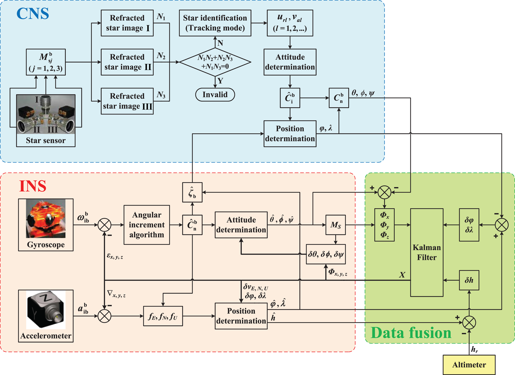
Figure 8. Flowchart of SIMU/triple star sensors deep integrated without refraction correction

In the CNS section, to ensure high-precision navigation in long-endurance flight, three (or two at least) FOVs should be available to detect stars, whose numbers of observed stars are N ₁, N ₂ and N ₃. Thus, the identified u_rl and the measured v_al can determine $\hat{\boldsymbol{C}}_{\rm i}^{\rm b}$ then calculate position parameters φ, λ and attitude parameters θ, ϕ, ψ through ${\hat{\boldsymbol{\zeta }}_{\rm b}}$ provided by INS.

Now, the new deep integrated method with refraction correction is shown as Figure 9.

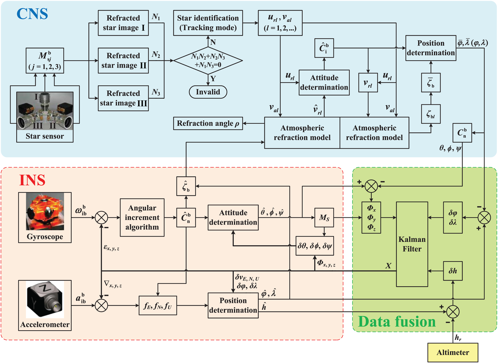
Figure 9. Flowchart of SIMU/triple star sensors deep integrated with refraction correction

Based on the atmospheric refraction model, $\hat{\boldsymbol{C}}_{\rm i}^{\rm b}$ determined by the identified u_rl and the corrected ${\hat{\boldsymbol{v}}_{\boldsymbol{r}l}}$ is more precise. The updated v_rl (calculated by $\hat{\boldsymbol{C}}_{\rm i}^{\rm b}$ and u_rl) and the measured v_al can then determine the corrected ζ_bl of each observed star. Calculate ${\bar{\boldsymbol{\zeta }}_{\rm b}}$ as

(35)\begin{equation}{\bar{\boldsymbol{\zeta }}_{\rm b}} = \frac{{\sum_{l = 1}^{{N_1} + {N_2} + {N_3}} {{\boldsymbol{\zeta }_{{\rm b}l}}} }}{{\left\|{\sum_{l = 1}^{{N_1} + {N_2} + {N_3}} {{\boldsymbol{\zeta }_{{\rm b}l}}} } \right\|}}\end{equation}

thus obtaining $\bar{\varphi }$, $\bar{\lambda }$ (i.e., φ, λ) followed with θ, ϕ, ψ.

Kalman filter is utilised to realise the data fusion (Pan et al., Reference Pan, Cheng, Liang, Yang and Wang2013). The navigation deviations are denoted as

(36)\begin{equation} \begin{cases} {\delta \theta = \hat{\theta } - \theta }\\ {\delta \phi = \hat{\phi } - \phi }\\ {\delta \psi = \hat{\psi } - \psi }\\ {\delta \varphi = \hat{\varphi } - \varphi }\\ \delta \lambda = \hat{\lambda } - \lambda \\ \delta h = \hat{h} - {h_r} \end{cases}\end{equation}

So the misalignment angles ${{\varPhi_x}}, {{\varPhi_y}}, {{\varPhi_z}}$ can be determined by (Zhu et al., Reference Zhu, Wang, Li, Che and Li2018)

(37)\begin{equation}\left[ {\begin{matrix} {{\varPhi_x}}\\ {{\varPhi_y}}\\ {{\varPhi_z}} \end{matrix}} \right] = {\boldsymbol{M}_{\boldsymbol{S}}}\left[ {\begin{matrix} {\delta \theta }\\ {\delta \phi }\\ {\delta \psi } \end{matrix}} \right] = \left[ {\begin{matrix} { {-} \cos \hat{\psi }}& { {-} \sin \hat{\psi }\cos \hat{\theta }}& 0\\ {\sin \hat{\psi }}& { - \cos \hat{\psi }\cos \hat{\theta }}& 0\\ 0& { {-} \sin \hat{\theta }}& 1 \end{matrix}} \right]\left[ {\begin{matrix} {\delta \theta }\\ {\delta \phi }\\ {\delta \psi } \end{matrix}} \right]\end{equation}

According to the error equations of SINS, build the 15-dimensional state model as follows

(38)\begin{equation}\boldsymbol{X} = {\left[ {\begin{array}{*{20}{c}} {\delta {v_E}}& {\delta {v_N}}& {\delta {v_U}}& {{\varPhi_x}}& {{\varPhi_y}}& {{\varPhi_z}}& {\delta \varphi }& {\delta \lambda }& {\delta h}& {{\varepsilon_x}}& {{\varepsilon_y}}& {{\varepsilon_z}}& {{\nabla_x}}& {{\nabla_y}}& {{\nabla_z}} \end{array}} \right]^{\rm T}}\end{equation}

where δv_E, δv_N, δv_U are velocity deviations; ε_x, ε_y, ε_z are gyroscope drifts; ∇_x, ∇_y, ∇_z are accelerometer biases. The state equation is

(39)\begin{align}\dot{\boldsymbol{X}} & = \boldsymbol{FX} + \boldsymbol{G}{\boldsymbol{W}_{{\bf SINS}}}\end{align}

(40)\begin{align}\boldsymbol{F} & = \left[ {\begin{array}{*{20}{c}} {{\boldsymbol{F}_{\boldsymbol{N}{\rm (9} \times {\rm 9)}}}}& {{\boldsymbol{F}_{\boldsymbol{S}{\rm (6} \times {\rm 6)}}}}\\ {{{\bf 0}_{{\rm 6} \times {\rm 9}}}}& {{{\bf 0}_{{\rm 9} \times {\rm 6}}}} \end{array}} \right]\end{align}

(41)\begin{align}\boldsymbol{G} & = \left[ {\begin{array}{*{20}{c}} {{{\bf 0}_{3 \times 3}}}& {\boldsymbol{C}_{\rm b}^{\rm n}}\\ { - \boldsymbol{C}_{\rm b}^{\rm n}}& {{{\bf 0}_{3 \times 3}}}\\ {{{\bf 0}_{{\rm 9} \times {\rm 3}}}}& {{{\bf 0}_{{\rm 9} \times {\rm 3}}}} \end{array}} \right]\end{align}

(42)\begin{align}{\boldsymbol{W}_{{\bf SINS}}}& = {\left[ {\begin{matrix} {{\omega_{\varepsilon x}}}& {{\omega_{\varepsilon y}}}& {{\omega_{\varepsilon z}}}& {{\omega_{\nabla x}}}& {{\omega_{\nabla y}}}& {{\omega_{\nabla z}}} \end{matrix}} \right]^{\rm T}}\end{align}

where ω_εx, ω_εy, ω_εz are gyroscope noises; ω _∇x, ω _∇y, ω _∇z are accelerometer noises. Non-zero elements of F_N are (Qin, Reference Qin2006; Li et al., Reference Li, Sheng, Zhang, Wu, Xu, Liu and Zhang2018)

\begin{align*}& \boldsymbol{F}_{\boldsymbol{N}}(1,1) =\frac{{{v_N}\;{\rm tan}\hat{\varphi } - {v_U}}}{{{R_N} + \hat{h}}}, \boldsymbol{F}_{\boldsymbol{N}}(1,2{\rm ) = 2}{\omega _{ie}}\sin \hat{\varphi } + \frac{{{v_E}\;{\rm tan}\hat{\varphi }}}{{R_N} + \hat{h}},\\& {\boldsymbol{F}_{\boldsymbol{N}}}(1,3) = - \left( {{\rm 2}{\omega_{ie}}\cos \hat{\varphi } + \frac{{{v_E}}}{{{R_N} + \hat{h}}}} \right), {\boldsymbol{F}_{\boldsymbol{N}}}(1,5) = - {f_U}, {\boldsymbol{F}_{\boldsymbol{N}}}(1,6) ={f_N}, \\& {\boldsymbol{F}_{\boldsymbol{N}}}(1,7{\rm ) = 2}{\omega _{ie}}({{v_U}\sin \hat{\varphi } + {v_N}\cos \hat{\varphi }} )+ \frac{{{v_E}{v_N}\;{\rm se}{{\rm c}^2}\hat{\varphi }}}{{{R_N} + \hat{h}}}, {\boldsymbol{F}_{\boldsymbol{N}}}(1,9) =\frac{{{v_E}{v_U} - {v_E}{v_N}\;{\rm tan}\hat{\varphi }}}{{{{({{R_N} + \hat{h}} )}^2}}}, \\& {\boldsymbol{F}_{\boldsymbol{N}}}(2,1) = - {\boldsymbol{F}_{\boldsymbol{N}}}(1,2), {\boldsymbol{F}_{\boldsymbol{N}}}(2,2) = - \frac{{{v_U}}}{{{R_M} + \hat{h}}}, {\boldsymbol{F}_{\boldsymbol{N}}}(2,3) = - \frac{{{v_N}}}{{{R_M} + \hat{h}}}, {\boldsymbol{F}_{\boldsymbol{N}}}(2,4) ={f_U},\\& {\boldsymbol{F}_{\boldsymbol{N}}}(2,6) = - {f_E}, {\boldsymbol{F}_{\boldsymbol{N}}}(2,7) = - \left( {{\rm 2}{\omega_{ie}}{v_E}\cos \hat{\varphi } + \frac{{v_E^2\;{\rm se}{{\rm c}^2}\hat{\varphi }}}{{{R_N} + \hat{h}}}} \right), \\& {\boldsymbol{F}_{\boldsymbol{N}}}(2,9) =\frac{{{v_N}{v_U}}}{{{{({{R_M} + \hat{h}} )}^2}}} + \frac{{v_E^2\;{\rm tan}\hat{\varphi }}}{{{{({{R_N} + \hat{h}} )}^2}}}, {\boldsymbol{F}_{\boldsymbol{N}}}(3,1{\rm ) = 2}{\omega _{ie}}\cos \hat{\varphi } + \frac{{2{v_E}}}{{{R_N} + \hat{h}}}, {\boldsymbol{F}_{\boldsymbol{N}}}(3,2) =\frac{{2{v_N}}}{{{R_M} + \hat{h}}},\\& {\boldsymbol{F}_{\boldsymbol{N}}}(3,4) = - {f_N}, {\boldsymbol{F}_{\boldsymbol{N}}}(3,5) ={f_E}, {\boldsymbol{F}_{\boldsymbol{N}}}(3,7) = - {\rm 2}{\omega _{ie}}{v_E}\sin \hat{\varphi },\\& {\boldsymbol{F}_{\boldsymbol{N}}}(3,9) = - \frac{{v_N^2}}{{{{({{R_M} + \hat{h}} )}^2}}} - \frac{{v_E^2}}{{{{({{R_N} + \hat{h}} )}^2}}}, {\boldsymbol{F}_{\boldsymbol{N}}}(4,2) = - \frac{1}{{{R_M} + \hat{h}}}, {\boldsymbol{F}_{\boldsymbol{N}}}(4,5) ={\omega _{ie}}\sin \hat{\varphi } + \frac{{{v_E}\;{\rm tan}\hat{\varphi }}}{{{R_N} + \hat{h}}},\\& {\boldsymbol{F}_{\boldsymbol{N}}}(4,6) = - {\omega _{ie}}\cos \hat{\varphi } - \frac{{{v_E}}}{{{R_N} + \hat{h}}}, {\boldsymbol{F}_{\boldsymbol{N}}}(4,9) =\frac{{{v_N}}}{{{{({{R_M} + \hat{h}} )}^2}}}, {\boldsymbol{F}_{\boldsymbol{N}}}(5,1) =\frac{1}{{{R_N} + \hat{h}}},\\& {\boldsymbol{F}_{\boldsymbol{N}}}(5,4) = - {\boldsymbol{F}_{\boldsymbol{N}}}(4,5), {\boldsymbol{F}_{\boldsymbol{N}}}(5,6) ={\boldsymbol{F}_{\boldsymbol{N}}}(2,3), {\boldsymbol{F}_{\boldsymbol{N}}}(5,7) = - {\omega _{ie}}\sin \hat{\varphi },\\& {\boldsymbol{F}_{\boldsymbol{N}}}(5,9) = - \frac{{{v_E}}}{{{{({{R_N} + \hat{h}} )}^2}}}, {\boldsymbol{F}_{\boldsymbol{N}}}{\rm (6},1) =\frac{{{\rm tan}\hat{\varphi }}}{{{R_N} + \hat{h}}}, {\boldsymbol{F}_{\boldsymbol{N}}}(6,4) = - {\boldsymbol{F}_{\boldsymbol{N}}}(4,6), {\boldsymbol{F}_{\boldsymbol{N}}}(6,5) = - {\boldsymbol{F}_{\boldsymbol{N}}}(2,3),\\& {\boldsymbol{F}_{\boldsymbol{N}}}(6,7) ={\omega _{ie}}\cos \hat{\varphi } + \frac{{{v_E}\;{\rm se}{{\rm c}^2}\hat{\varphi }}}{{{R_N} + \hat{h}}}, {\boldsymbol{F}_{\boldsymbol{N}}}{\rm (6},9) = - \frac{{{v_E}\;{\rm tan}\hat{\varphi }}}{{{{({{R_N} + \hat{h}} )}^2}}}, {\boldsymbol{F}_{\boldsymbol{N}}}(7,2) = - {\boldsymbol{F}_{\boldsymbol{N}}}(4,2),\\& {\boldsymbol{F}_{\boldsymbol{N}}}(7,9) = - {\boldsymbol{F}_{\boldsymbol{N}}}(4,9), {\boldsymbol{F}_{\boldsymbol{N}}}(8,1) =\frac{{{\rm sec}\hat{\varphi }}}{{{R_N} + \hat{h}}}, {\boldsymbol{F}_{\boldsymbol{N}}}{\rm (8},7) ={v_E}\;{\rm tan}\hat{\varphi }{\boldsymbol{F}_{\boldsymbol{N}}}{\rm (8},1),\\& {\boldsymbol{F}_{\boldsymbol{N}}}(8,9) ={\boldsymbol{F}_{\boldsymbol{N}}}(5,9)\;{\rm sec}\hat{\varphi }, {\boldsymbol{F}_{\boldsymbol{N}}}(9,3) =1,\end{align*}

where R_M is the main radius of curvature of the meridian; R_N is the main radius of curvature of prime vertical; ω_ie is the rotational angular velocity of the Earth.

(43)\begin{equation}{\boldsymbol{F}_{\boldsymbol{S}}} = \left[ {\begin{array}{*{20}{c}} {{{\bf 0}_{3 \times 3}}}& {\boldsymbol{C}_{\rm b}^{\rm n}}\\ { - \boldsymbol{C}_{\rm b}^{\rm n}}& {{{\bf 0}_{3 \times 3}}} \end{array}} \right]\end{equation}

Build the six-dimensional measurement model as follows

(44)\begin{equation}\boldsymbol{Z} = {\left[ {\begin{array}{*{20}{c}} {{\varPhi_x}}& {{\varPhi_y}}& {{\varPhi_z}}& {\delta \varphi }& {\delta \lambda }& {\delta h} \end{array}} \right]^{\rm T}}\end{equation}

The measurement equation is

(45)\begin{align}\boldsymbol{Z} & = \boldsymbol{HX} + {\boldsymbol{V}_{\boldsymbol{m}}}\end{align}

(46)\begin{align}\boldsymbol{H} & = \left[ {\begin{array}{*{20}{c}} {{{\bf 0}_{6 \times 3}}}& {{\boldsymbol{I}_{6 \times 6}}}& {{{\bf 0}_{6 \times 6}}} \end{array}} \right]\end{align}

where V_m is measuring noise.

Generally, the data output rate of the SIMU is higher than the star sensor. During the interval of CNS output, INS alone calculates and updates the navigation parameters and matrix P in Kalman filter. Otherwise, data fusion proceeds and the final filtering result X will be feedback to INS and compensate for the state errors. Then X will be reset to zero until the next filtering moment.

5. Simulation verification and analysis

In this section, simulation of the zenith error range located by different zenith distances will be given first. Then, both the static simulations of CNS with the coplanar distribution scheme (assigned as Scheme 1) and the triangular distribution scheme (assigned as Scheme 2), as well as the dynamic simulations of SINS/CNS deep integrated with Scheme 2, will be discussed.

5.1 Simulation of the zenith error range

According to Figure 2, assign μ_a as the celestial equator, u_r orienting to the vernal equinox, $({\hat{\alpha }_\zeta },{\hat{\delta }_\zeta })$ as the right ascension and declination of $\hat{\boldsymbol{\zeta }}$, then ζ(z_r, 0). Obviously,

\[\left\{ \begin{array}{@{}l} \left[ {\begin{matrix} {\cos {{\hat{\delta }}_\zeta }\cos {{\hat{\alpha }}_\zeta }}& {\cos {{\hat{\delta }}_\zeta }\sin {{\hat{\alpha }}_\zeta }}& {\sin {{\hat{\delta }}_\zeta }} \end{matrix}} \right]{\cdot} {\left[ {\begin{matrix} 1& 0& 0 \end{matrix}} \right]^{\rm T}} = \cos {{\hat{z}}_r}\\ \left[ {\begin{matrix} {\cos {{\hat{\delta }}_\zeta }\cos {{\hat{\alpha }}_\zeta }}& {\cos {{\hat{\delta }}_\zeta }\sin {{\hat{\alpha }}_\zeta }}& {\sin {{\hat{\delta }}_\zeta }} \end{matrix}} \right]{\cdot} {\left[ {\begin{matrix} {\cos {z_r}}& {\sin {z_r}}& 0 \end{matrix}} \right]^{\rm T}} = \cos \Delta \zeta \\ {\rm sgn}({{\hat{\delta }}_\zeta }) = {\rm sgn}(\beta ) \end{array} \right.\]

Therefore, combined with Equation (12),

\[\begin{cases} {{\hat{\alpha }}_\zeta } = {\rm arctan}({{\rm tan}{{\hat{z}}_r}\cos \beta } )\\ {{\hat{\delta }}_\zeta } = {\rm sgn}(\beta ){\rm arccos}\sqrt {{\rm si}{{\rm n}^2}{{\hat{z}}_r}\;{\rm co}{{\rm s}^2}\beta + {\rm co}{{\rm s}^2}{{\hat{z}}_r}} \end{cases}\]

Setting Δu_a = 1′′, h = 15 km, then the zenith error ranges in various conditions are shown in Figure 10.

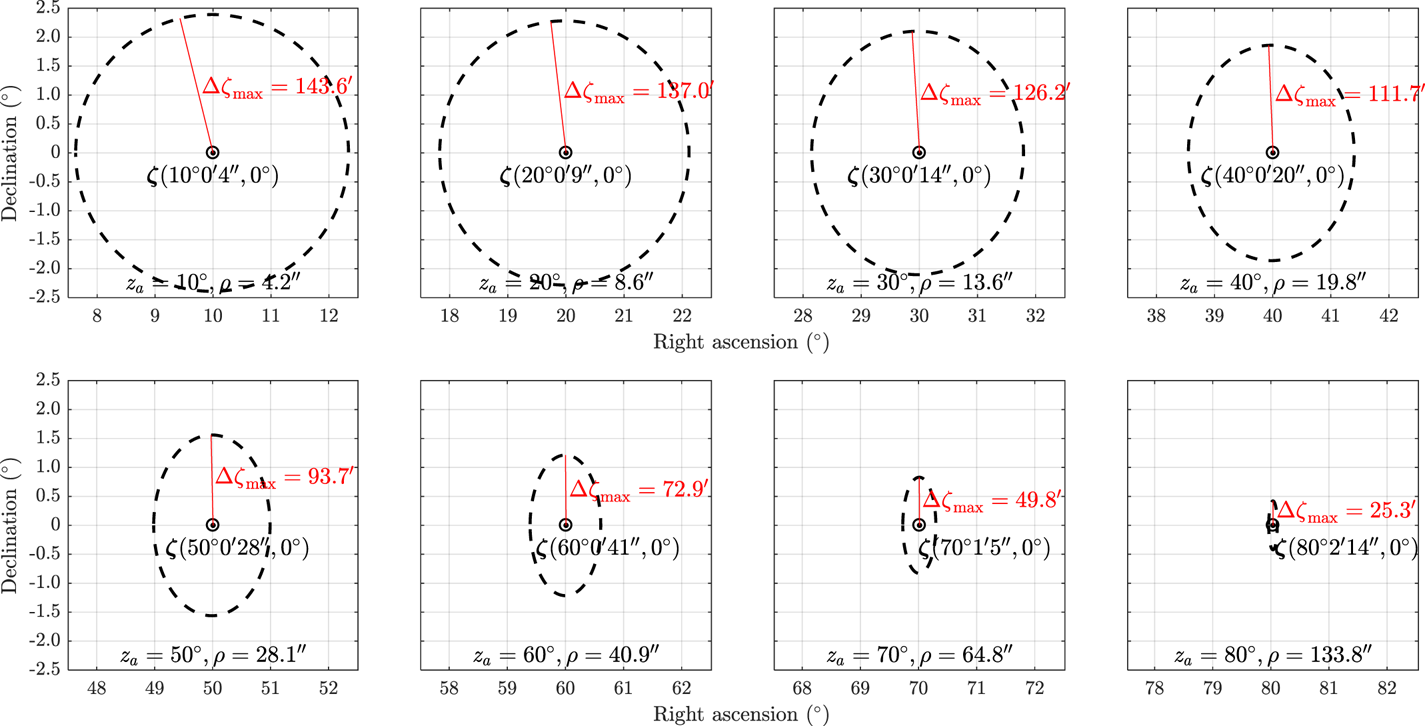
Figure 10. Zenith error ranges with different zenith distances

It can be seen that both the error range and Δζ _max decrease with increasing zenith distance. However, even if Δζ is about 25′ (e.g. z_a = 80°, Δζ _max = 25⋅3′), the position error will be up to 46 km (one arc minute gives an error in coordinates of approximately one nautical mile, i.e., 1.852 km) on the Earth's surface, let alone the larger Δu_a in actual flight.

It should be noted that refraction effects in the vicinity of the horizon are more complicated (Yu et al., Reference Yu, Cao, Tang, Luo and Zhao2015). Therefore, the optimal navigation star for positioning should be located high enough above the horizon.

5.2 Static simulation of CNS

In static simulations without any measurement noise, the Monte Carlo method with 200 times independent repeated experiments will be used to calculate the root mean square error (RMSE) of navigation parameters. Setting h = 15 km, α_s = 70°, corresponding α_A = 1⋅009 (The Purple Mountain Observatory, 2021), $\boldsymbol{C}_{\rm i}^{\rm e}$ = I_3×3.

5.2.1 Precision analysis with Scheme 1

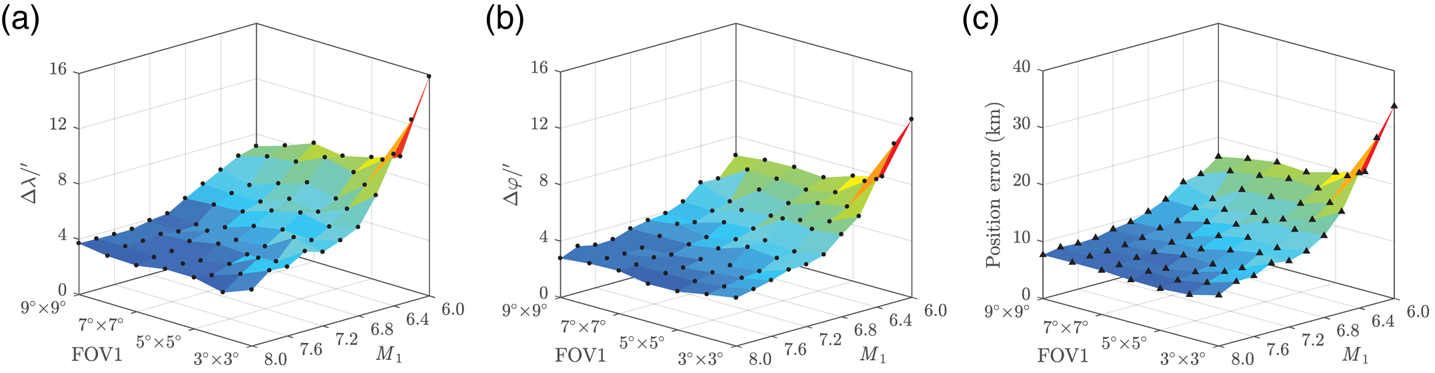
On the condition that the Z _b axis orients to the zenith, λ, φ and ψ are randomly generated. According to Fan and Li's study (Reference Fan and Li2011), the initial limiting magnitude (denoted as M) of star sensors I, II and III was set as 8⋅0, with FOV 3° × 3°. Then, the FOV of Sensor I was changed from 3° × 3° to 9° × 9°, and M ₁ from 8⋅0 to 6⋅0. Sensors II and III remain unchanged. The simulation results are shown in Figures 11–13.

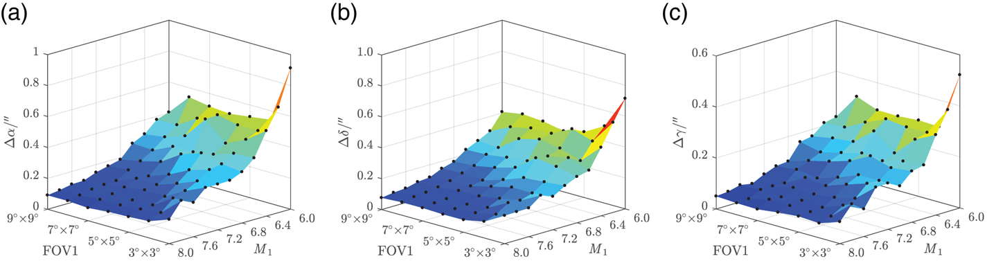
Figure 11. Absolute attitude RMSE: (a) right ascension error (b) declination error (c) roll error

Figure 12. Position RMSE: (a) longitude error (b) latitude error (c) total position error

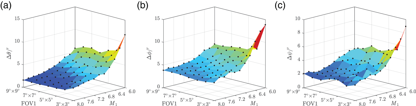
Figure 13. Relative attitude RMSE: (a) pitch error (b) roll error (c) yaw error

Obviously, with the decrease of M ₁ and FOV1, which indicate fewer stars being detected, both the attitude error and position error tend to increase. Besides, as shown in Figure 10, ρ < 4⋅2′′ when z_a < 10°, h = 15 km. Although the absolute attitude RMSE is strictly limited within 1′′, the position RMSE and relative attitude RMSE, however, are still big enough especially for positioning, let alone with manoeuvre or measurement noise in calculation. This indicates that Scheme 1 has low engineering feasibility.

5.2.2 Precision and loss function analyses with Scheme 2

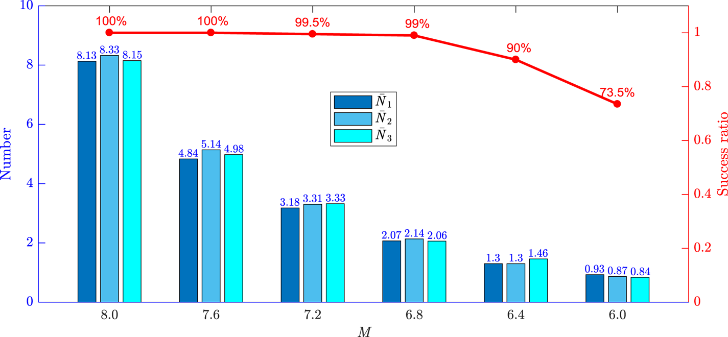
Sensors I, II and III with FOV 3° × 3° are equivalent. M_j (j = 1, 2, 3) is reduced from 8⋅0 to 6⋅0. The observation results are shown in Figure 14 where the success ratio of attitude determination is the percentage that at least two stars can be observed in 200 samples. It can be seen that both the number of observed stars and the success ratio decrease with reducing M. Ensuring the detectivity of each star sensor is vitally important in actual flight. Therefore, ${M_j} \ge 6.4,{\bar{N}_j} > 1$ (j = 1, 2, 3) with success ratio higher than 90% should be satisfied in practice to ensure real-time accuracy, as set out in Section 5.3.

Figure 14. Mean number of observed stars and success ratio of attitude determination

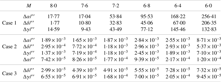
For each sample where attitude was successfully determined, the attitude determination method without refraction corrected is assigned as Case 1, the method with only two FOVs available with refraction corrected is assigned as Case 2 and the method with all three FOVs available with refraction corrected as Case 3. Thereinto, the nominal location is given in Case 2 and Case 3. The simulation results of the absolute attitude error are shown in Figure 15 and Table 1.

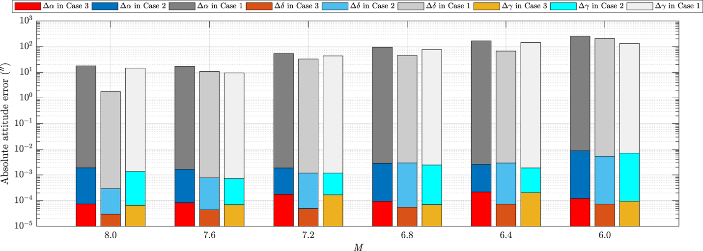
Figure 15. Attitude RMSE in the three cases

Table 1. Attitude RMSE in the three cases

Obviously, the attitude precision determined by Case 1 is rough. Case 2 is worse than Case 3, despite its computational attitude RMSE with finite bit capacity of the processor in algorithm simulation having already been equal to zero under the ideal conditions. In the long-endurance flight condition, Case 2 can be considered as an alternative.

The next step is to verify the feasibility of the conjugate gradient iterative method mentioned in Section 3.2. Set M = 8⋅0. Assign λ_{b 0} = 151⋅22° and φ_{b 0} = 85⋅39°, solved by a random flight status as the nominal location. Then, separately plot the loss function in the domain around (λ_{b 0}, φ_{b 0}) with attitudes determined by Case 1 and Case 3, as in Figure 16, where a_l = 1/(N ₁ + N ₂ + N ₃) (l = 1,…, N ₁ + N ₂ + N ₃). It can be seen that the loss function is non-convex when the rough attitude (Case 1) is given. Only if the precise attitude (Case 3) is acquired can $({\hat{\lambda }_b},{\hat{\varphi }_b})$ converge to (λ_{b 0}, φ_{b 0}) with loss function minimised. However, this is difficult to realise in application with refraction influence.

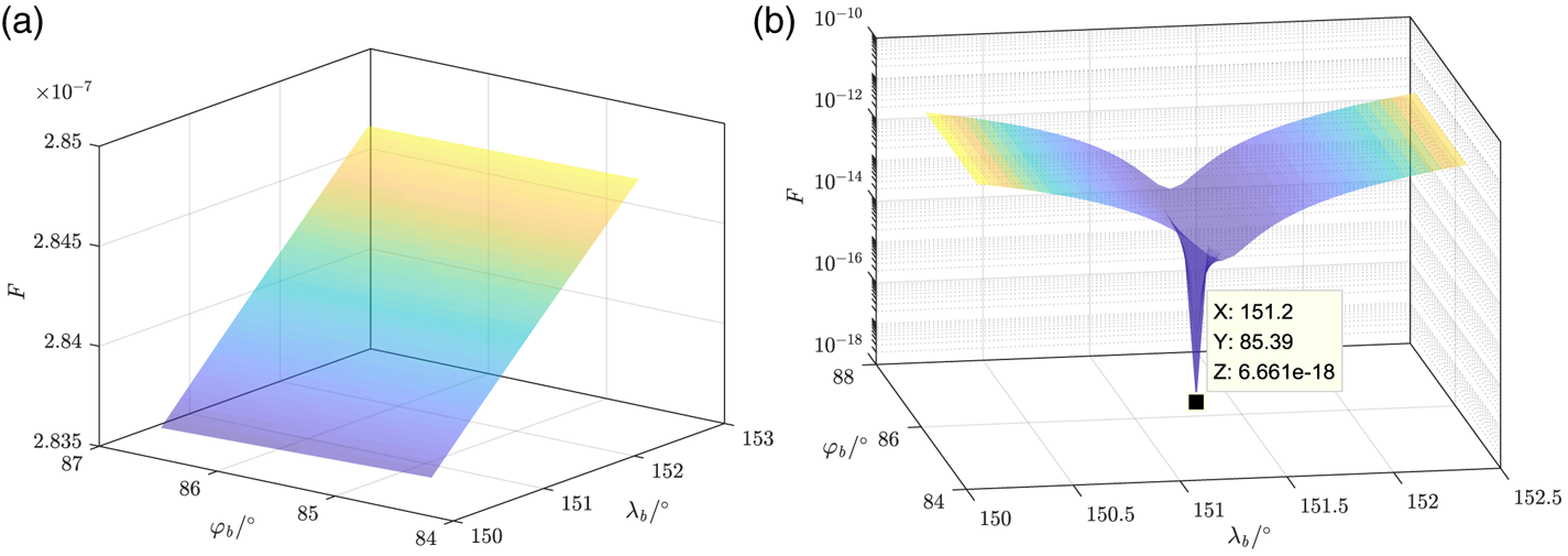
Figure 16. Loss function simulation: (a) attitude determined by Case 1, (b) attitude determined by Case 3

5.3 Dynamic simulation of SINS/CNS

5.3.1 Environment settings

A simplified nominal flight trajectory with manoeuvring in the stratosphere is designed to verify the integrated method. One flight cycle is set at 4 h with time nodes t ₀, t ₁, t ₂, t ₃, t ₄ at intervals of 1 h. The UAV's velocity is set at 60 m/s constantly orienting to the Y _b axis (attack angle is 0°, sideslip angle is 0°) and the initial real (nominal) kinematic parameters satisfy (φ_r(t ₀), λ_r(t ₀)) = (40°, 120°), h_r(t ₀) = 15 km, θ_r(t ₀) = ϕ_r(t ₀) = 0°, ψ_r(t ₀) = 90°. The initial Greenwich hour angle of the vernal equinox A _ϒ(t ₀) = 59⋅03°. The designed kinematic parameters vary as shown in Figure 17.

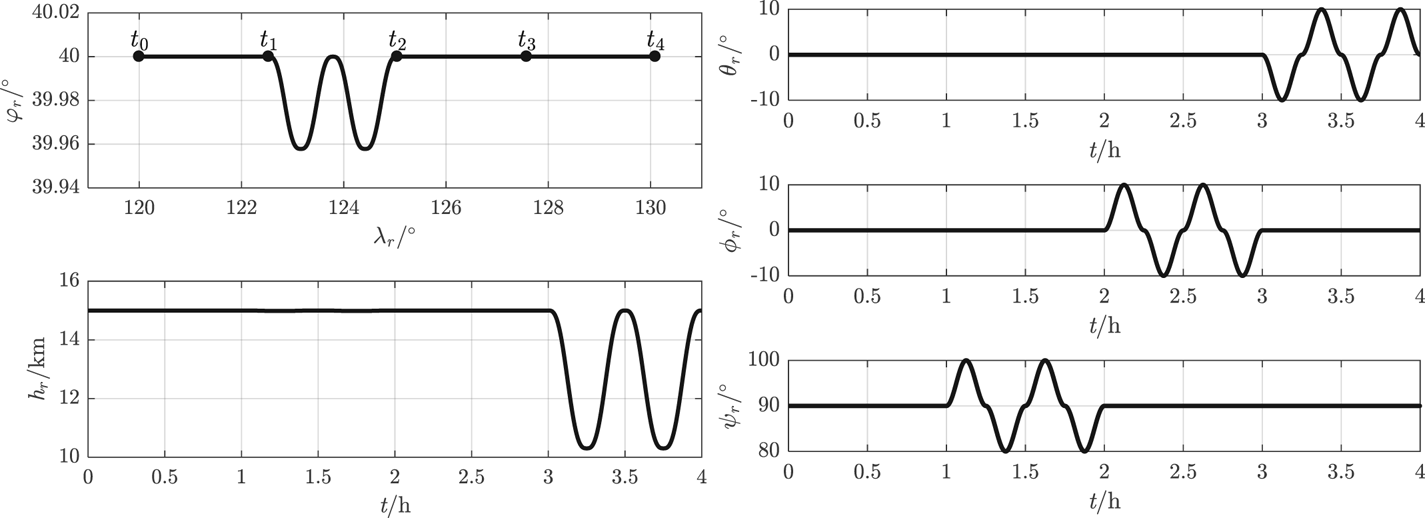
Figure 17. Real kinematic parameters of UAV

The simulation parameters of various navigational apparatus are shown in Table 2. In addition, α_s = 70°, α_A = 1⋅009, FOV 3° × 3° and δv_{E ,N,U}(t ₀) = 0⋅1 m/s, $\varPhi$_{x ,y,z}(t ₀) = 1′′, δφ(t ₀) = δλ(t ₀) = 1′′, δh(t ₀) = 50 m.

Table 2. Simulation parameters of navigational apparatus

5.3.2 Flight simulation within 4 h

In one 4 h flight cycle, the constant M = 8⋅0. For the proposed deep integrated method with refraction corrected and the traditional method with refraction uncorrected, the real-time simulation errors of navigation parameters are estimated as shown in Figures 18–21. The RMSEs of the navigation parameters are shown in Table 3.

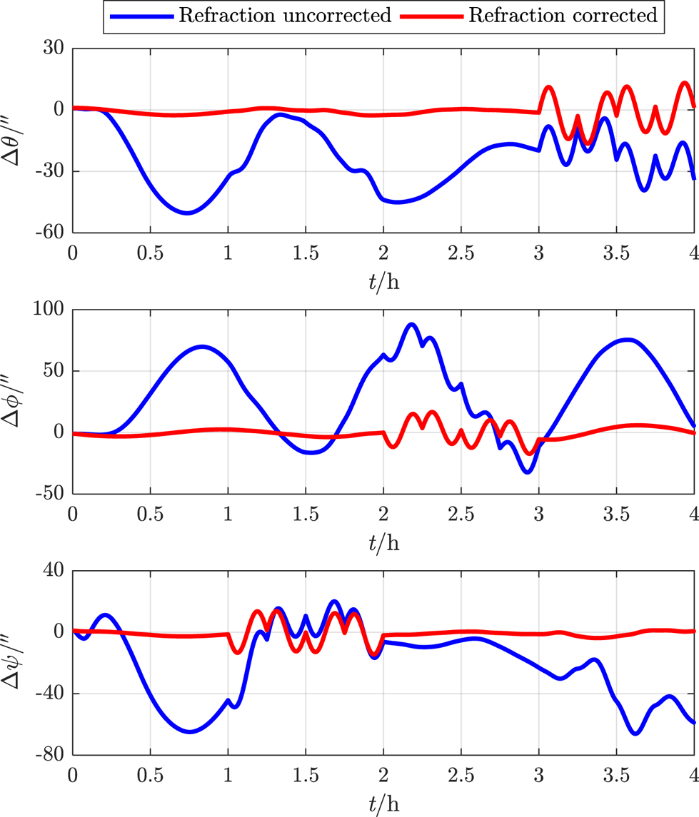
Figure 18. Attitude error within 4 h

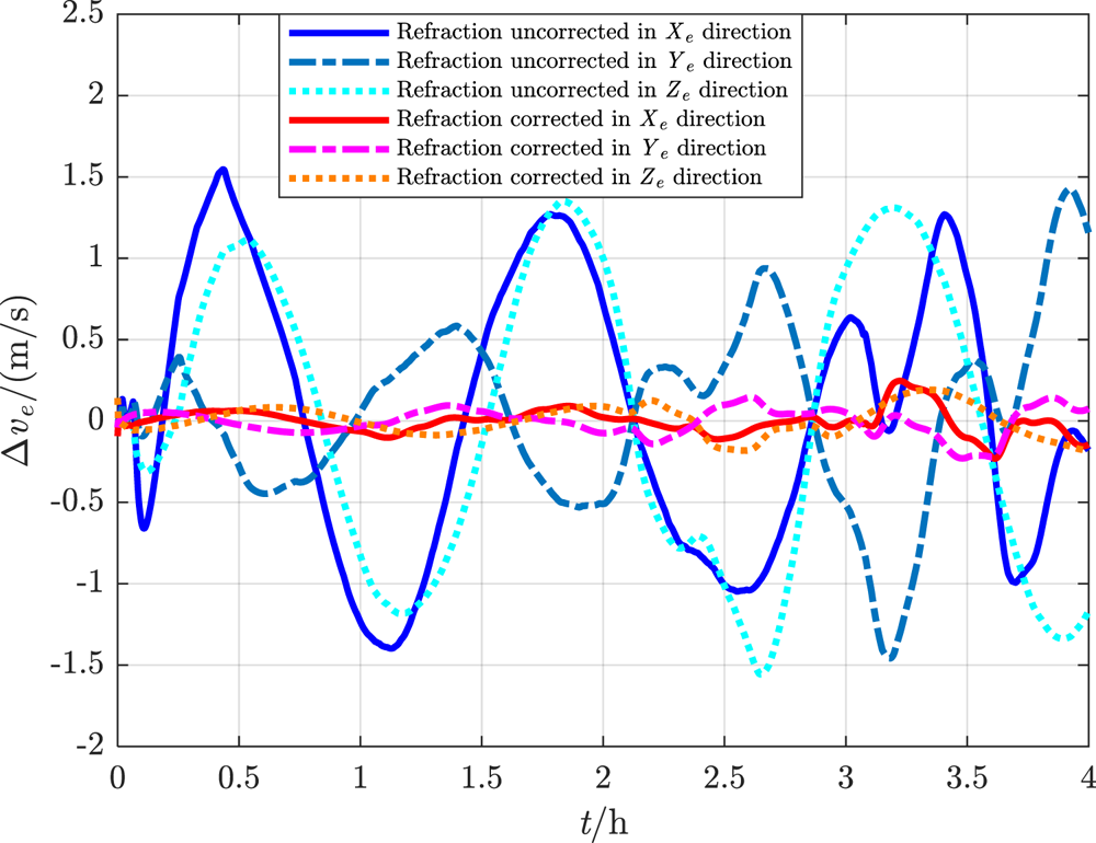
Figure 19. Velocity error within 4 h

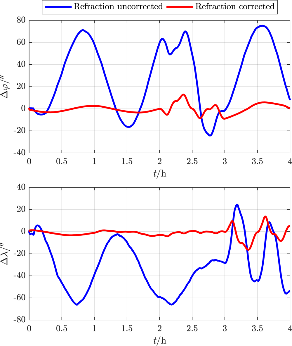
Figure 20. Geographical coordinate error within 4 h

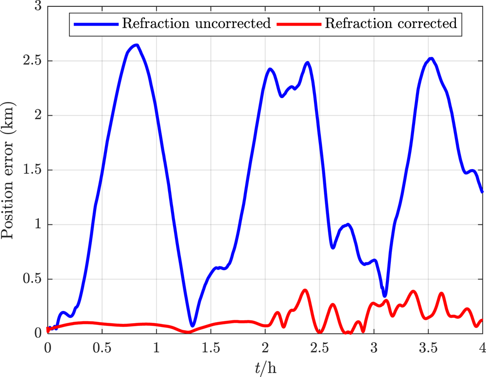
Figure 21. Total position error within 4 h

Table 3. Navigation parameter RMSE of 4 h flight

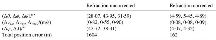
It can be seen that, under the influence of atmospheric refraction, all the navigation error data of the traditional integrated method without correction oscillate or even diverge, while the proposed deep integrated method with correction can eliminate the influence of tight coupling between attitude and position on navigation accuracy, and thus effectively restrain navigation error within a limited range even in manoeuvring flight.

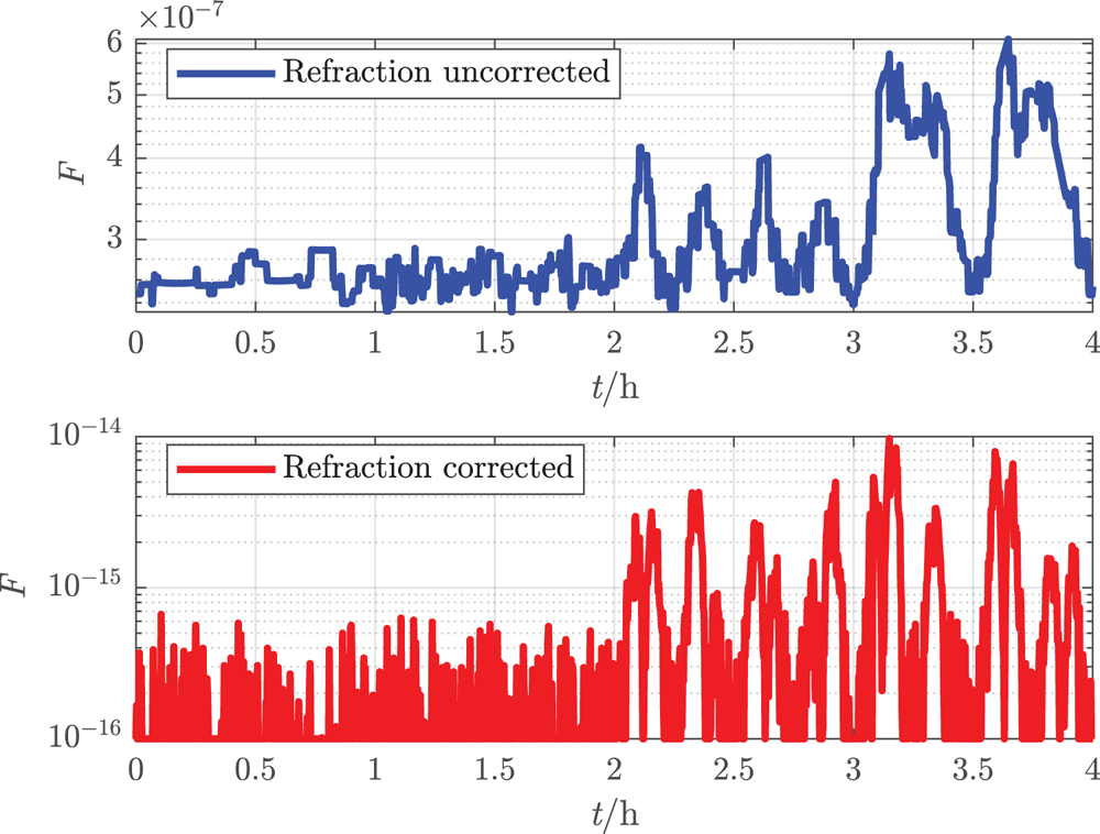
The real-time loss functions of the two methods are plotted in Figure 22. Although the orders of magnitude are so small that the numerical value may overflow in calculation, it does verify that smaller function value indicates higher navigation accuracy.

Figure 22. Loss function within 4 h

5.3.3 Flight simulation within 24 h

For the purpose of simulating the decrease of limiting magnitude with enhancing atmospheric background radiation in long-endurance flight, M is respectively set to 8⋅0, 7⋅7, 7⋅4, 7⋅1, 6⋅8 and 6⋅5 in six continuous flight cycles (i.e., 24 h flight). The final results of the proposed deep integrated method are shown in Figure 23.

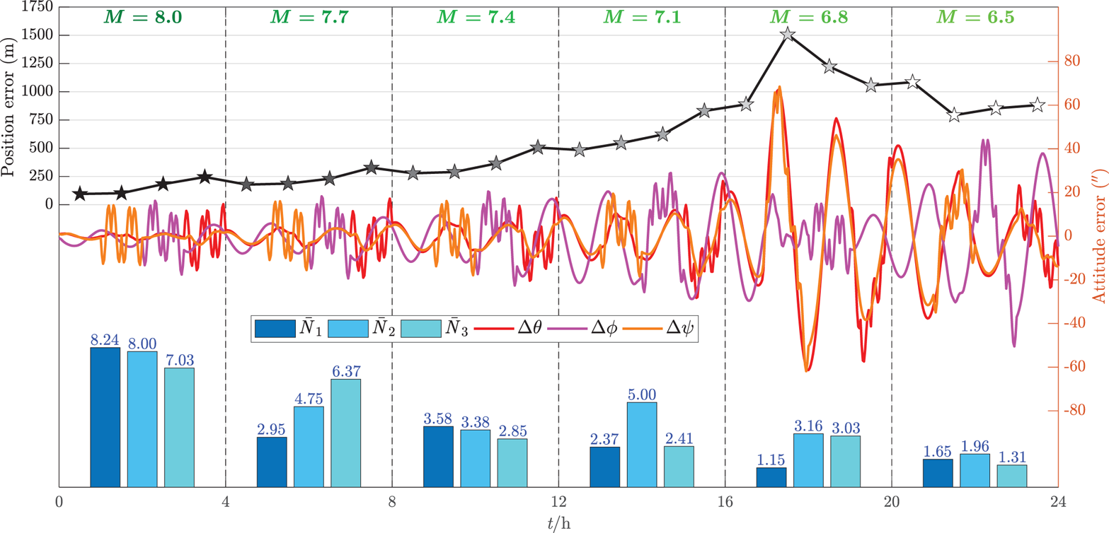
Figure 23. Navigation error and mean number of observed stars within 24 h

It can be seen that, with the decrease of limiting magnitude together with the number of observed stars among different flight cycles, the navigation accuracy tends to be worse. Nevertheless, the position RMSE in each hour can still be restrained within 1⋅5 km and the attitude real-time error can be restrained within 70′′ even after 24 h manoeuvring flight with limiting magnitude above 6⋅5. Obviously, the proposed method can overcome the problem of unreliability of CNS operating by itself. When better conditions are satisfied, e.g., all the sensors are available to detect stars all the time, higher navigation accuracy can be achieved, and thus the cruising ability of the UAV can be ensured.