


1. INTRODUCTION
The nautical mile is a special unit employed for marine and air navigation to express distance. The value 1,852 m was adopted by the First International Extraordinary Hydrographic Conference, Monaco 1929, under the name “International nautical mile” (The International System of Units (SI), 2006). The International Nautical Mile (INM) is used in navigational devices such as logs and radars.
The constant INM is an approximation of the Sea Mile (SM) defined as the length of one minute of arc, measured along the meridian of the Earth, in the latitude of the position. As the Earth is not a perfect sphere and in geodesy is defined as an ellipsoid, its actual length varies with latitude.
Navigational devices such as, for example, logs and radars are calibrated in INMs. On the other hand, distances which can be measured on nautical charts are in SMs which means that two different measures meet together on nautical charts.
This difference is up to ±0·5% and such simplification has been necessary and quite justified compared to the accuracy of navigation at the time of the definition of the INM. But the question arises now – are these simplifications still justified in modern navigation?
2. GEODETIC SOLUTIONS
The SM is defined on an ellipsoid and therefore the application of solutions of the problems known in geodesy as the direct and the inverse geodetic problems should be applied.
Lenart (Reference Lenart2011) and Lenart (Reference Lenart2013) present a set of procedures for calculating distances and azimuths on an ellipsoid of revolution for orthodromes and loxodromes. The orthodrome in this paper (which literally means straight line) is defined as the path of the shortest distance on any surface, for example, a plane, a spheroid or an ellipsoid and the latter is used in these calculations.
In formal notations:
 $$\hbox{S} = \hbox{IGP}\lpar \varphi_{1}\comma \; \lambda_{1}\comma \; \varphi_{2}\comma \; \lambda_{2}\rpar $$
 $$\hbox{C}_{\rm gs}\comma \; \hbox{C}_{\rm ge} = \hbox{IGP}\lpar \varphi_{1}\comma \; \lambda_{1}\comma \; \varphi_{2}\comma \; \lambda_{2}\rpar $$
 $$\hbox{S}_{\rm lx} = \hbox{LX}\lpar \varphi_{1}\comma \; \lambda_{1}\comma \; \varphi_{2}\comma \; \lambda_{2}\rpar $$
 $$\hbox{C}_{\rm glx} = \hbox{LX}\lpar \varphi_{1}\comma \; \lambda_{1}\comma \; \varphi_{2}\comma \; \lambda_{2}\rpar $$
 $$\varphi_{2}\comma \; \lambda_{2} = \hbox{DGP}\lpar \varphi_{1}\comma \; \lambda_{1}\comma \; \hbox{S}\comma \; \hbox{C}_{\rm gs}\rpar $$
 $$\hbox{C}_{\rm ge} = \hbox{DGP}\lpar \varphi_{1}\comma \; \lambda_{1}\comma \; \hbox{S}\comma \; \hbox{C}_{\rm gs}\rpar $$
where P1(φ1, λ1) and P2(φ2, λ2) are the departure point and the destination point, respectively, S is the orthodromic distance, Cgs is the Course Over the Ground (COG) at the departure point of the orthodrome and Cge is the COG at the destination point of the orthodrome, Slx is the loxodromic distance and Cglx is the loxodromic COG.
IGP is the procedure of the Inverse Geodetic Problem solution which calculates orthodromic distance and COG at the departure point from the coordinates of the departure and the destination points. LX is a similar procedure for loxodromic calculations. DGP is the procedure of the Direct Geodetic Problem solution which calculates coordinates and COG of the destination point from coordinates and COG of the departure point and the orthodromic distance.
In this paper these procedures, with results based on full accuracy Sodano's solutions (Sodano, Reference Sodano1958; 1965; Reference Sodano1967) on the WGS-84 (World Geodetic System) reference ellipsoid (as in Lenart (Reference Lenart2011) and Lenart (Reference Lenart2013)) will be used in general formal form but any other geodetic solutions of comparable or better accuracies can be applied, such as the widely used, in other than navigation applications, algorithms of Vicenty (1975) and Kearney (Reference Kearney2013). Sodano's solutions have been selected because they are very satisfactory for marine and air navigation accuracy for any length of geodesics with simple rigorous non-iterative procedures.
3. SEA MILE ANALYSIS
A simplified formula for the sea mile between latitudes φ and φ + 1′ (for example, Weintrit, Reference Weintrit2015) is widely used:
 $$\hbox{S}_{\rm SM} \approx \hbox{a}_{0} [ 1 - \hbox{e}^{2} \lpar 1 + 3\cos2\varphi\rpar /4] \ \hbox{arc}\, 1^{\prime} $$
where a0 is the semi-major axis of the reference ellipsoid and e is the eccentricity of the reference ellipsoid.
More correct and more accurate for the latitude φ is the following procedure (in accordance with Equation (1)):
 $$\hbox{S}_{\rm SM} = \hbox{IGP} \lpar \varphi - 0{\cdot}5^{\prime}\comma \; 0\comma \; \varphi + 0{\cdot}5^{\prime}\comma \; 0\rpar \, \hbox{or for}\, \varphi = 90^{\circ}\, \hbox{S}_{\rm SM} = \hbox{IGP} \lpar 89^{\circ}59{\cdot}5^{\prime}\comma \; 0\comma \; 89^{\circ}59{\cdot}5^{\prime}\comma \; 180^{\circ}\rpar $$
or similar to Equation (7):
 $$\hbox{S}_{\rm SM} = \hbox{IGP}\lpar \varphi\comma \; 0\comma \; \varphi + 1^{\prime}\comma \; 0\rpar \hbox{ or for }\varphi = 90^{\circ}\, \hbox{S}_{\rm SM} = \hbox{IGP}\lpar 90^{\circ}\comma \; 0\comma \; 89^{\circ}59^{\prime}\comma \; 180^{\circ}\rpar $$
It can be found that (Weintrit, Reference Weintrit2015):
 $$\hbox{S}_{\rm SM} \approx \hbox{M arc }1^{\prime} $$
where M is the radius of curvature in the meridian given by:
 $$\hbox{M}=\displaystyle{{\hbox{a}_0 \lpar 1-\hbox{e}^2\rpar }\over{\sqrt {\lpar 1-\hbox{e}^2\sin ^2\varphi \rpar ^3}}} $$
Table 1 presents results of Equation (8) and errors of Equations (7), (9) and (10) referenced to Equation (8) and these are illustrated in Figures 1–4.
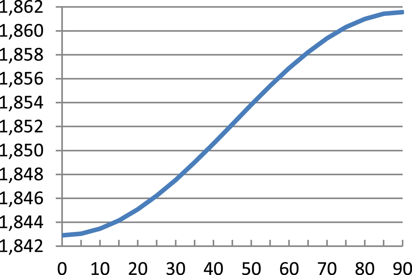
Figure 1. Sea mile – Equation (8) [m].
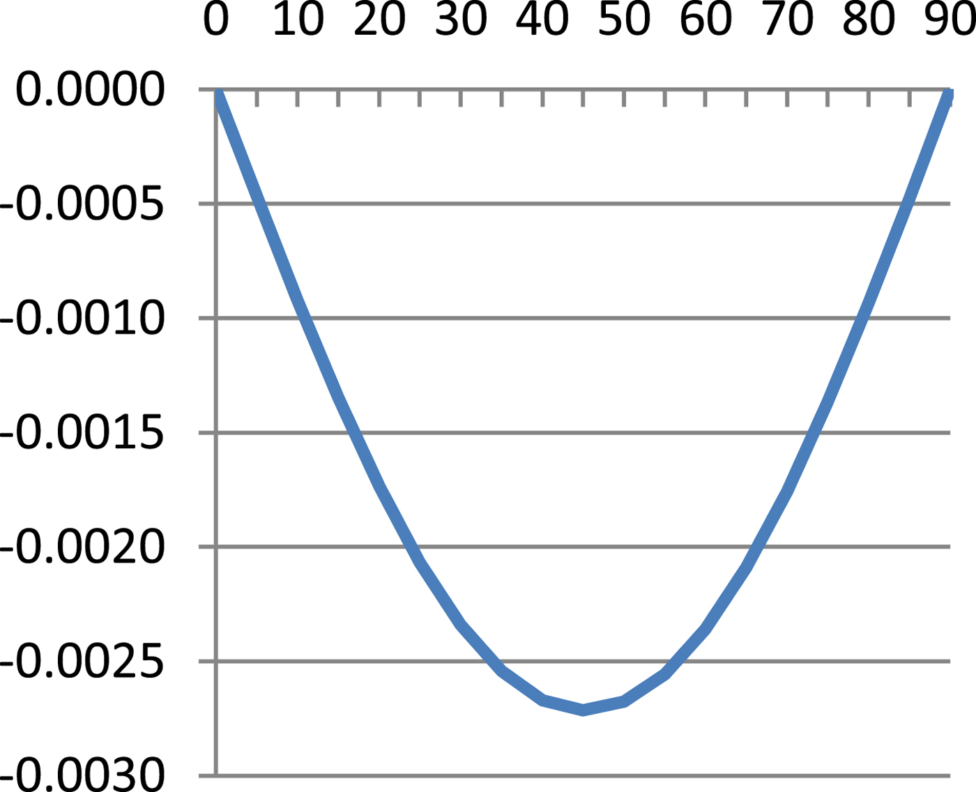
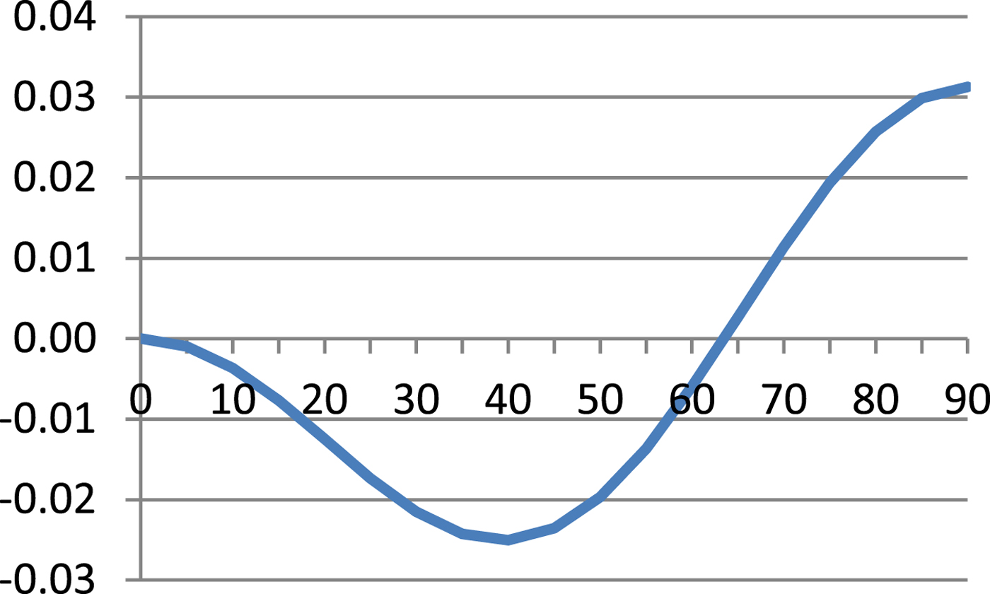
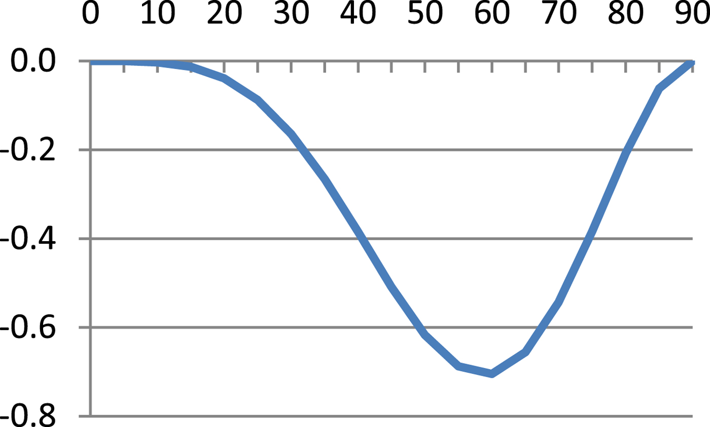
Table 1. Sea mile, comparison of errors and derivative
As can be seen from Table 1 and Figures 1–4, errors of Equation (9) are from 0 to −0·27 cm, errors of Equation (7) are from −2·51 cm to +3·13 cm and errors of Equation (11) are from 0 to −70·49 cm. It is evident that between Equation (8) and Equation (9) there is a very small difference, Equation (7) is quite a good approximation of Equation (8) and Equation (7) is simpler and more accurate then Equation (10).
The INM was chosen as the integer number of metres closest to the mean sea mile at latitude 45° hence:
 $$\hbox{S}_{\rm SM} =1852_{-9{\cdot}57}^{+9{\cdot}10}\quad \hbox{m}\approx 1852\, \hbox{m}\pm 0{\cdot}5\% $$
and the biggest differences are at the poles and the equator - the latter is more important in marine navigation because the poles are rather inaccessible for marine navigation (other than underwater navigation at the North Pole).
From Equation (7) the derivative is given by:
 $$\displaystyle{{\hbox{dS}_{\rm SM}}\over{\hbox{d}\varphi}}=\displaystyle{{3}\over{2}}\hbox{a}_0 \hbox{e}^2\sin 2\varphi \cdot \hbox{arc}\, 1^{\prime} $$
which reaches an extreme at φ = 45° (Table 1, Figure 5):
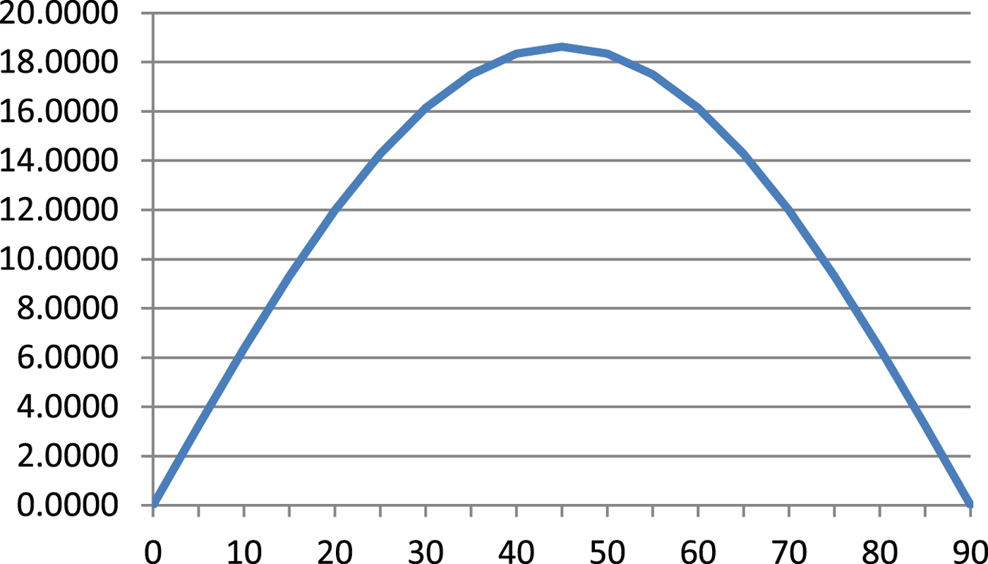
Figure 5. Derivative – Equation (13)
 $$\displaystyle{{\hbox{dS}_{\rm SM}}\over{\hbox{d}\varphi}}\max =\displaystyle{{3}\over{2}}\hbox{a}_0 \hbox{e}^2\ \hbox{arc}\, 1^{\prime}$$
and consequently:
 $$\displaystyle{{\hbox{dS}_{\rm SM}}\over{\hbox{d}\varphi}}\max \lpar 1^{\prime}\rpar =\displaystyle{{\hbox{dS}_{\rm SM}}\over{\hbox{d}\varphi}}\max \cdot \hbox{arc}\ 1^{\prime}=0{\cdot}54\, \hbox{cm}/1^{\prime} $$
 $$\displaystyle{{\hbox{dS}_{\rm SM}}\over{\hbox{d}\varphi}}\max \lpar 1^{\circ}\rpar =\displaystyle{{\hbox{dS}_{\rm SM}}\over{{\rm d}\varphi}}\max \cdot \hbox{arc}\ 1^{\circ}=32{\cdot}52\, \hbox{cm}/1^{\circ} $$
4. POSITION FIXING
As has been stated in Section 1, navigational devices such as logs and radars are calibrated in INMs. On the other hand, distances which can be measured on nautical charts are in SMs – two different measures meet together. Thus errors in manual position fixing, such as in dead reckoning or radar position fixes, of to ±0·5% of the distance, can be expected. Manual position fixing is still required as a backup for electronic position fixing.
Modern navigational devices are more accurate than simple mechanical or electromechanical devices in terms of the definition of the INM. What is more, these devices are microprocessor controlled and optionally switched calibration in sea miles is possible.
In logs, current latitude should be entered from, for instance a Global Positioning System (GPS) receiver via a NMEA input (National Marine Electronics Association – NMEA is a specification commonly used for communication between marine navigation devices) and current SSM can be calculated with regard to Equation (7) or from the table of SSM as a function of latitude taking into consideration Equations (14)–(16). Fortunately, the extreme of the derivative is at the longitudes near the smallest difference between the INM and the SM.
Radars and Automatic Radar Plotting Aids (ARPAs) are often connected with position fixing devices and for manual radar position fixes only the distance from a Variable Range Marker (VRM) should be optionally calculated in SM according to:
 $$\hbox{D}_{\rm SM} =\displaystyle{{\hbox{D}_{\rm INM} \cdot 1852}\over{\hbox{S}_{\rm SM}}} $$
where DSM is the distance measured in sea miles, DINM is the distance measured in INM and SSM is from Equation (7) or from the table as in logs.
It is also possible to produce an equivalent graphical solution on future large-scale paper nautical charts by printing a double scale in SM and INM.
5. ORTHODROMIC DISTANCE IN SEA MILES
Orthodromic distances on the ellipsoid (for example from Equation (1)) are calculated in metres (since the ellipsoid WGS-84 is defined in metres) and results - where necessary - are converted to and from INM.
For orthodromic distances in SM the following iterative procedure can be used:
 $$\eqalign{& \hbox{S}=\hbox{IGP}\lpar \varphi_{1}\comma \; \lambda_{1}\comma \; \varphi_{2}\comma \; \lambda_{2}\rpar \cr & \hbox{C}_{\rm gsi}=\hbox{IGP}\lpar \varphi_{1}\comma \; \lambda_{1}\comma \; \varphi_{2}\comma \; \lambda_{2}\rpar \cr & \hbox{D}_{\rm SM}=0 \cr & \hbox{S}_{\rm i}=0 \cr & \varphi_{i}=\varphi_{1}\semicolon \; \lambda_{i}=\lambda_{1} \cr & \hbox{DO} \cr & \quad \varphi_{\rm 2i}\comma \; \lambda_{\rm 2i}=\hbox{DGP}\lpar \varphi_{\rm i}\comma \; \lambda_{\rm i}\comma \; \hbox{S}_{\rm SM}\lpar \varphi_{\rm i}\rpar \comma \; \hbox{C}_{\rm gsi}\rpar \cr & \quad \hbox{C}_{\rm gei}=\hbox{DGP}\lpar \varphi_{\rm i}\comma \; \lambda_{\rm i}\comma \; \hbox{S}_{\rm SM}\lpar \varphi_{\rm i}\rpar \comma \; \hbox{C}_{\rm gsi}\rpar \cr & \quad \hbox{S}_{\rm i}=\hbox{S}_{\rm i}+\hbox{S}_{\rm SM}\lpar \varphi_{\rm i}\rpar \cr & \quad \hbox{D}_{\rm SM}=\hbox{D}_{\rm SM}+1 \cr & \quad \varphi_{\rm i}=\varphi_{\rm 2i}\semicolon \; \lambda_{\rm i}=\lambda_{\rm 2i} \cr & \quad \hbox{C}_{\rm gsi}=\hbox{C}_{\rm gei} \cr & \hbox{LOOP UNTIL S}_{\rm i}>\hbox{S} \cr & \hbox{D}_{\rm SM}=\hbox{D}_{\rm SM}+\lpar \hbox{S}-\hbox{S}_{\rm i}\rpar /\hbox{S}_{\rm SM}\lpar \varphi_{\rm i}\rpar } $$
where DSM is the distance in SMs and SSM(φi) is the length of the SM from Equation (7) at latitude φi.
In this procedure, with the direct geodetic problem solution, the consecutive points on the orthodrome in steps of the length of the SM at the current latitude are calculated and concurrently the distance from the departure point is counted in metres as Si and the number of SM is counted as DSM. The procedure ends when Si is bigger than S – the orthodromic distance - and finally DSM is corrected for the last step.
Equation (7) is simplified and errors of this simplification in the above procedure are integrated. These errors can be easily revealed for meridional orthodromes because for these orthodromes the correct value is equal to the difference of latitudes in minutes. As can be seen from Table 2 these errors are less then ±0·02 SM even when the first two positions in this table are for latitudes for which the error Equation (8)–Equation (7) has extremes (Figure 3).
Table 2. Errors of the procedure for orthodromes in sea miles
6. LOXODROMIC DISTANCE IN SEA MILES
The loxodromic distance in Equation (3) is calculated from:
 $$\hbox{S}_{\rm lx} =\left\vert\displaystyle{{\hbox{S}_{\rm M} \lpar \varphi_1 \comma \; \varphi_2 \rpar }\over{\cos \hbox{C}_{\rm glx}}}\right\vert $$
where SM(φ1, φ2) is the meridian distance between latitudes φ1 and φ2 and this distance in SM can be calculated (as in Section 5) as the difference of latitudes in minutes. Therefore, the procedure for the loxodromic distance is as follows:
 $$\eqalign{& \hbox{IF }\varphi_{1} = \varphi_{2}\ \hbox{THEN} \cr & \quad \hbox{S}_{\rm lx}\, [ \hbox{SM}] =\displaystyle{{\hbox{S}_{\rm lx}\, \hbox{[ m] }}\over{\hbox{S}_{\rm SM} \lpar \varphi_1\rpar }} \cr & \hbox{ELSE } \cr & \quad \hbox{S}_{\rm lx}\, [ \hbox{SM}] =\left\vert\displaystyle{{\lpar \varphi_2 -\varphi_1 \rpar \cdot 60}\over{\cos \hbox{C}_{\rm glx}}}\right\vert \cr & \hbox{ENDIF}} $$
In the case φ1 = φ2, the loxodrome is latitudinal at a constant latitude.
7. EXEMPLARY REAL ROUTES
The first exemplary route is from Cape Horn (S 55°59′, W 67°17′) to Sydney (S 33°50′, E 151°17°). This route is intentionally at higher latitudes to magnify all differences. For this route:
 $$\eqalign{& \hbox{S} = 5{\comma \; }077{\cdot}7\, \hbox{INM} = 5{\comma \; }064{\cdot}9\, \hbox{SM -- difference}\, {-}0{\cdot}25{\percnt } \cr & \hbox{S}_{\rm lx} = 6{\comma \; }063{\cdot}8\, \hbox{INM} = 6{\comma \; }063{\cdot}2\, \hbox{SM -- difference}\, {-0\cdot01\%}}$$
Although the maximum latitude for this orthodrome is high for marine navigation (73 · 1°), the mean latitude for this loxodrome is near 45° hence the small difference between the length of the loxodrome in INM and SM.
The second exemplary route - intentionally at lower latitudes - is from Manta in Ecuador (S 00°56′, W 80°43′) to Jayapura on New Guinea (S 02°32′, E 140°43′). The results are:
 $$\eqalign{& \hbox{S} = 8{\comma \; }320{\cdot}8\, \hbox{INM} = 8{\comma \; }361{\cdot}5\, \hbox{SM -- difference}\, 0{\cdot}47{\percnt } \cr & \hbox{S}_{\rm lx}=8{\comma \; }325{\cdot}4\, \hbox{INM} = 8{\comma \; }366{\cdot}4\, \hbox{SM -- difference}\, 0{\cdot}49{\%}}$$
8. CONCLUSIONS
Simplification of the sea mile dependent on latitude to the constant international nautical mile was justified in 1929 when it was defined. Modern navigation devices are more accurate and more powerful and consequently this simplification is no longer necessary. The proposed algorithms for the calculation of sea miles in different sailing methods can be easily incorporated in modern microprocessor controlled navigational devices, so that both miles can exist in the same device. An equivalent graphical solution on selected nautical charts is also proposed.


