


1. INTRODUCTION
Laser Detection And Ranging (LADAR) devices have been widely used in robotics and unmanned systems. There are various types of LADARs, including Two-Dimensional (2D) and Three-Dimensional (3D) scanners, and 3D flash LADARs. Compared with 3D scanners and flash LADARs, 2D scanners tend to require less space, weight or power to achieve the same operational range, which makes them more suitable for small robotic systems, such as small Unmanned Aerial Vehicles (UAVs). The navigation algorithms discussed in this work are based on 2D laser scanners.
Various types of 2D LADAR-based navigation have been designed for UAVs operating in an urban environment, indoors, or in other situations where Global Navigation Satellite Systems (GNSS) are unavailable. In these applications, the navigation system could rely on Simultaneous Localisation and Mapping (SLAM) solutions (Dissanayake et al., Reference Dissanayake, Newman, Clark, Durrant-Whyte and Csorba2001; Bailey and Durrant-Whyte, Reference Bailey and Durrant-Whyte2006). In addition to the platform position and orientation, a SLAM solution also estimates the location of landmarks, or a grid map of the environment (Thrun et al., Reference Thrun, Burgard and Fox2005). LADAR measurements can be aided with an odometer, an Inertial Navigation System (INS) or an Inertial Measurement Unit (IMU). The solution can be implemented using a Kalman Filter (Guivant and Nebot, Reference Guivant and Nebot2001), a particle filter (Montemerlo and Thrun, Reference Montemerlo and Thrun2003) or other filter types. For example, in an Extended Kalman Filter (EKF), the 2D or 3D locations of all the landmarks can be included in the state space. Such an implementation results in computational time complexity of O(K 2), with K landmarks in the state space. Various types of optimisation have been proposed to make the solution more efficient. For example, the complexity of a particle filter-based FastSLAM is O(Nlog K) when using N particles (Montemerlo and Thrun, Reference Montemerlo and Thrun2003). In a real-world application, the size of the map may be constantly growing. This inevitably results in increasing computational complexity and latency, which raises major concerns in real-time systems. For autonomous control and guidance of a UAV, the on board flight control system relies on frequent and prompt updates to maintain control of the vehicle velocity, altitude and orientation, for which large latencies cannot be tolerated.
A more efficient solution can be found by estimating location and orientation with respect to a fixed map. For example, the widely used Monte Carlo Localisation (MCL) is based on particle filters and a priori grid maps (Dellaert et al., Reference Dellaert, Fox, Burgard and Thrun1999). MCL has a complexity of O(N) when using N particles, and it does not increase with the map size.
Another alternative is to obtain relative displacement and rotation between consecutive scans, which can be directly extracted from LADAR measurements without using any map. Although it does not provide a positioning solution in a global reference frame directly, it can be used as an odometry update to INS/IMU. One possible implementation is based on Iterative Closest Point matching, as introduced in Chen and Medioni (Reference Chen and Medioni1991), Besl and Mckay (Reference Besl and Mckay1992), Menq et al. (Reference Menq, Yau and Lai1992) and Champleboux et al. (Reference Champleboux, Lavallee, Szeliski and Brunie1992), and more recently in Vadlamani and Uijt de Haag (Reference Vadlamani and Uijt de Haag2006). The complexity of these approaches is also independent of the map size.
Point cloud or grid map-based approaches would both be applicable in man-made and natural environments since they do not require visibility of certain features or characteristics to be present in the data. However, they both require 3D LADARs in order to estimate position and orientation in a 3D coordinate frame.
Since this work targets urban and indoor scenarios, it is safe to assume that linear and planar features will be abundant. Most of these features are likely to be extracted from stationary structures. Zhang and Faugeras (Reference Zhang and Faugeras1991) demonstrated that the translation and rotation can be estimated using repeated observation of lines in a 3D point cloud. 2D LADARs can be used to estimate a 3D solution as well (Shen et al. Reference Shen, Michael and Kumar2011; Grzonka et al., Reference Grzonka, Grisetti and Burgard2012). Soloviev et al. (Reference Soloviev, Bates and Van Graas2007) first introduced a tightly-coupled, linear feature-based LADAR-IMU approach for 2D odometry, which is further extended to a 3D solution based on planar surfaces (Soloviev and Uijt de Haag, Reference Soloviev and Uijt de Haag2010b), where planar surfaces can be observed by introducing intentional motion to a 2D LADAR. Based on the same concept, a robust and efficient odometry estimation approach using planar features will be presented in this work.
One of the challenges faced with most LADAR-based navigation solutions is a dynamic environment. For example, if some of the scan points or features are non-stationary, they should be considered as outliers, and should not be included in the solution. Otherwise, they will result in biases in both the displacement and rotation estimates, which poses a threat to the integrity of navigation. The term “integrity” is used to quantify the trust that can be put in the solution, which is critical to the safety of manned and unmanned aviation. Recently, the integrity of LADAR navigation has started to gain more attention (Joerger et al., Reference Joerger, Jamoom, Spenko and Pervan2016). As a step toward integrity protection, outlier detection algorithms have to be implemented. It has been shown that RANdom SAmple Consensus (RANSAC) (Fischler and Bolles, Reference Fischler and Bolles1981) can be used to detect outliers for various types of LADAR solutions (Fontanelli et al., Reference Fontanelli, Ricciato and Soatto2007; Lu et al., Reference Lu, Hu, Uchimura, Xie, Xiong, Xiong, Liu and Hu2009). RANSAC exploits the redundancy in a large measurement group, which is not the case when there are only a few planar features available. The Receiver Autonomous Integrity Monitoring (RAIM) method (Farrell and Van Graas, Reference Farrell and Van Graas1991) and its variations represent another type of outlier detection algorithm. RAIM was originally designed to flag and eliminate erroneous ranging measurements in a GNSS receiver, and it does not require a large sample size. The outlier detection algorithm discussed in this paper is comparable to GNSS RAIM, which was first presented in Zhu and Uijt de Haag (Reference Zhu and Uijt de Haag2015).
In Section 2 of this paper, the proposed displacement and rotation estimation algorithms will be introduced. The outlier detection methods for both algorithms are presented in Section 3. Section 4 includes results and discussion of simulation and field tests, followed by a brief summary.
2. 3D NAVIGATION WITH A 2D LADAR
First, let us consider the 2D LADAR navigation problem: (a) the LADAR-IMU system moves from the origin of an X-Y coordinate system to a new location (x u , y u ), (b) the LADAR makes a scan of a fixed surface, for example, a wall, (c) a LADAR line detection is executed by one of the methods discussed in Borges and Aldon (Reference Borges and Aldon2004) and the lines are associated with line segments extracted at the previous time epoch, (d) the shortest distance to the new scan line is found. This distance changes from ρ i to ρ j between two scan epochs as illustrated in Figure 1.
Figure 1. Displacement measurement using a 2D LADAR (all measurements referenced to the body frame at epoch i). n i is the normal vector of the wall with angle ψ i .
Since the wall is stationary, the change in distance reflects the motion of the LADAR. However, the orientation and location of the LADAR could change during a scan, which can be compensated by using IMU data. After this compensation, the change in distance can then be used to estimate (x u , y u ), referenced to the body frame at epoch i.
 $$\rho_{i}-\rho_{j}=\cos (\psi_{i})x_{u}+\sin (\psi_{i})y_{u}={\bf{n}}_{i}\cdot \Delta {\bf{R}}$$
where
 $\Delta {\bf{R}}=(x_{u},y_{u})^{T}$
.
$\Delta {\bf{R}}=(x_{u},y_{u})^{T}$
.
 $\Delta {\bf{R}}$
can be explicitly solved with multiple non-parallel scan lines using, for example, a Least Squares estimator:
$\Delta {\bf{R}}$
can be explicitly solved with multiple non-parallel scan lines using, for example, a Least Squares estimator:
 $$\Delta \bf{R}=({\bf{H}}^{{\rm T}}\bf{H})^{-1}{\bf{H}}^{\rm{T}}{\bf{Y}}$$
where the measurement Y is a M by 1 vector,
 ${\bf{Y}}=[(\rho_{i1}-\rho_{j1}),(\rho_{i2}-\rho_{j2}),\ldots,(\rho_{iM}-\rho_{jM})]^{T}$
and geometry matrix H consists of M normal vectors
${\bf{Y}}=[(\rho_{i1}-\rho_{j1}),(\rho_{i2}-\rho_{j2}),\ldots,(\rho_{iM}-\rho_{jM})]^{T}$
and geometry matrix H consists of M normal vectors
 ${\bf{H}}=[\bi{n}_{i1}^{T},\bi{n}_{i2}^{T},\ldots \bi{n}_{iM}^{T}]^{T}$
.
${\bf{H}}=[\bi{n}_{i1}^{T},\bi{n}_{i2}^{T},\ldots \bi{n}_{iM}^{T}]^{T}$
.
A correct solution from Equation (2) relies on the assumption that all the lines are from stationary surfaces. A moving line would break the integrity of the solution. An initial investigation on the detection and removal of a moving line can be found in Soloviev and Uijt de Haag (Reference Soloviev and Uijt de Haag2010a).
To achieve 3D navigation, a 2D LADAR can be rotated by a servo-motor to scan at different elevation angles, as suggested in Soloviev and Uijt de Haag (Reference Soloviev and Uijt de Haag2010b). Thus, it becomes possible to obtain two or more 3D scans on the same planar surface. As shown in Figure 2, the displacement and rotation between two epochs are represented with
 ${\Delta \bf{R}}$
and a direction cosine matrix
${\Delta \bf{R}}$
and a direction cosine matrix
 ${\bf{C}}_{j}^{i}$
respectively. The principle of estimating
${\bf{C}}_{j}^{i}$
respectively. The principle of estimating
 ${\Delta \bf{R}}$
is almost identical to that of the 2D displacement problem, i.e., Equation (2), with the exception of replacing the lines with planar surfaces.
${\Delta \bf{R}}$
is almost identical to that of the 2D displacement problem, i.e., Equation (2), with the exception of replacing the lines with planar surfaces.
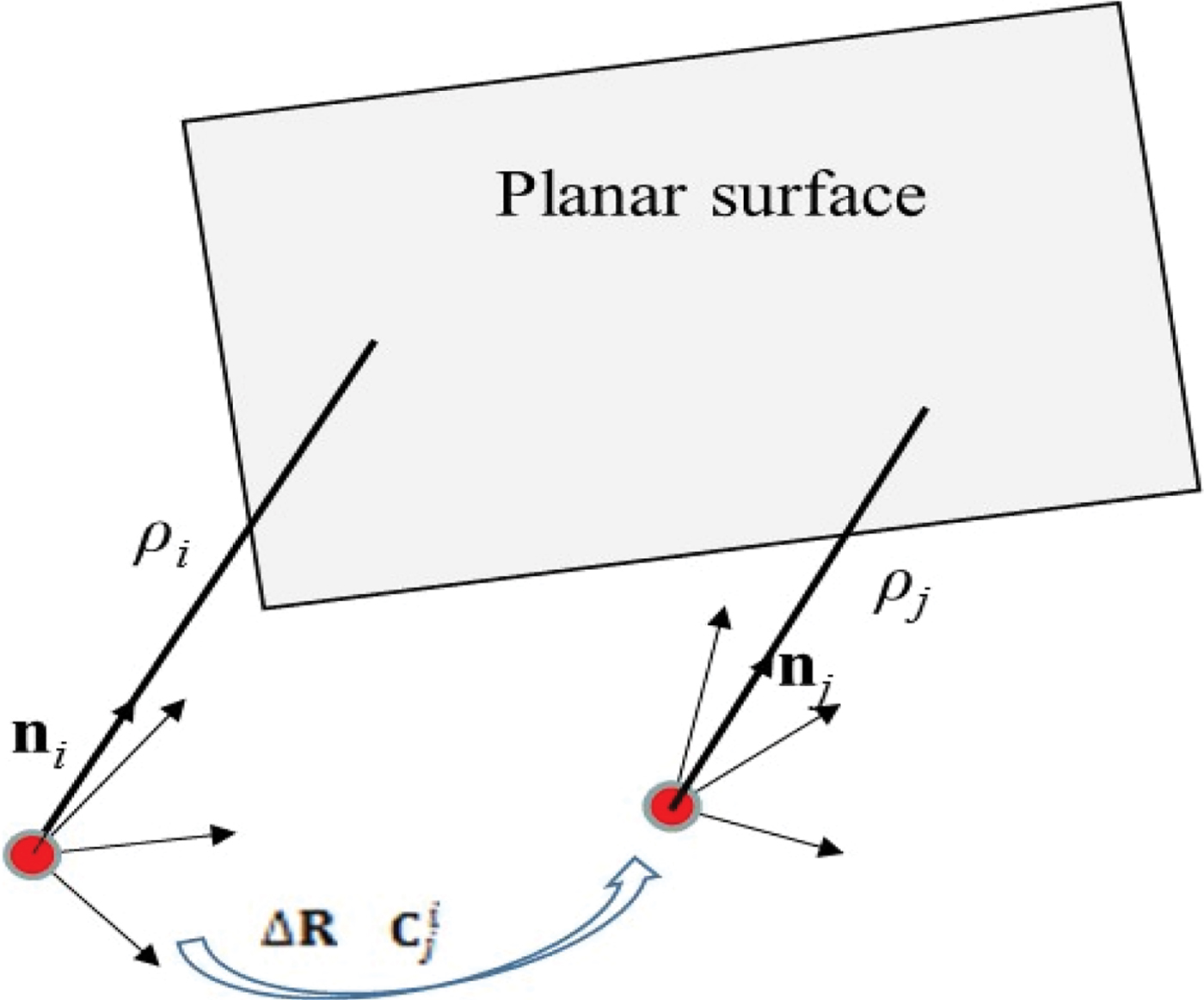
Figure 2. Displacement and rotation measurement based on a planar surface. n
i
and ρ
i
the normal vector and the distance observed at epoch i, whereas n
j
and ρ
j
are from epoch j. The displacement and rotation are denoted with Δ R and
 ${\bf{C}}_{j}^{i}$
respectively.
${\bf{C}}_{j}^{i}$
respectively.
The planar surfaces are also used to solve for 3D orientation change. Although a notional solution was proposed in Soloviev and Uijt de Haag (Reference Soloviev and Uijt de Haag2010b), an algorithm that is optimised for real-time implementation, possibly for a small embedded system, is yet to be detailed. The normal vectors to planar surfaces have to be estimated from the scan lines. Since the scans are all measured in the body frame, rotation of the body frame orientation would transform the normal vectors:
 $${\bf{C}}_{j}^{i}{\bf{n}}_{j}={\bf{n}}_{i}$$
A minimum set of two non-parallel planar surfaces are required for the three Degrees-Of-Freedom (DOF) solution, since every normal vector constrains the DOF by two. A linearized solution of
 ${\bf{C}}_{j}^{i}$
is summarised as follows.
${\bf{C}}_{j}^{i}$
is summarised as follows.
-
1) Obtain an initial estimate of rotation from the IMU prediction,
 $(\hat{\hbox{C}}_{j}^{i})_{0}$
-
2) The initial estimate may be off from the true
${\bf{C}}_{j}^{i}$
:
(4)where
$$(\hat{\hbox{C}}_{j}^{i})_{0}=(\delta {\bf{C}}_{j}^{i}){\bf{C}}_{j}^{i}$$
$\delta {\bf{C}}_{j}^{i}\approx {\bf{I}}+\Delta \bf{\Omega}\times$
, and
$\Delta \bf{\Omega}\times$
is the skew symmetric matrix of small angular errors in x, y and z directions, and
$\Delta \bf{\Omega}=[\Delta \varphi ,\Delta \theta,\Delta \psi]^{T}$
.
-
3) A normal vector from frame i can be rotated into frame j by using
$\hat{\bf{n}}_{j1}=(\hat{\bf{C}}_{j}^{i})_{0}{\bf{n}}_{i1}$
. It can be compared against the normal vector measured in frame j, and the difference is due to orientation errors
$\Delta \bf{\Omega}$
, i.e.
(5)Measurements from multiple planar surfaces can be combined into:
$$\hat{\bf{n}}_{j1}-{\bf{n}}_{j1}=(\hat{\bf{C}}_{j}^{i})_{0}{\bf{n}}_{i1}-{\bf{n}}_{j1}=\Delta \bf{\Omega} \times {\bf{n}}_{i1}$$
(6)where
$$\Delta \bf{n}={\bf{H}}_{\Omega}\Delta \bf{\Omega}$$
$\Delta {\bf{n}}$
is a 3M by one vector, and
${\bf{H}}_{\Omega}$
is a 3M by three matrix:
$$\Delta \bf{n}=\left[\matrix{(\hat{\bf{C}}_{j}^{i})_{0}{\bf{n}}_{i1}-{\bf{n}}_{j1}\cr (\hat{\bf{C}}_{j}^{i})_{0}{\bf{n}}_{i2}-{\bf{n}}_{j2}\cr \ldots\cr (\hat{\bf{C}}_{j}^{i})_{0}{\bf{n}}_{iM}-{\bf{n}}_{jM}}\right],\quad {\bf{H}}_{\bf{\Omega}}=\left[\matrix{{\bf{n}}_{i1}\times \cr {\bf{n}}_{i2}\times \cr \ldots\cr {\bf{n}}_{iM}\times}\right]$$
-
4) Solve for
$\Delta {\bf{\Omega}}$
using an Ordinary Least Squares solution:
(7)
$$\Delta \hat{\Omega}=({\bf{H}}_{{\Omega }}^{T}{\bf{H}}_{{\Omega }})^{-1}{\bf{H}}_{{\Omega }}^{T}\Delta {\bf{n}}$$


The association of planar features from one epoch to the next is based on the normal vector and location, and it can even be aided with IMU prediction when necessary. Therefore, feature correspondence is not of major concern in the proposed method.
3. 3D NAVIGATION WITH OUTLIER DETECTION
A moving object will cause a bias in both displacement and rotation, and both solutions will manifest different sensitivity levels to such motion. Detection of the moving object depends on the observability of a bias among several noisy measurements.
Obviously, residuals can be observed if the solutions in Equation (2) or Equation (7) are over-determined. In order to reliably flag an outlier, a set of detection criteria will be set based on the models of measurements and uncertainty. To protect the integrity of a real-time solution, outlier detection has to be performed on an epoch-to-epoch basis. It can be more challenging than solving the same problem in SLAM, because there are neither states nor covariance matrices associated with the planar surfaces in the filter. Further, only a small number of planar surfaces are required in this solution, which is a better fit for RAIM-like outlier detection algorithms.
3.1. Measurement Extraction
Two lines can uniquely define a planar surface, and it is equivalent to using only one line and an extra point outside this line. Figure 3 shows an example of two scan lines on a planar surface. Let there be L points on the first scan, Line1, and L′ points on the second scan, Line2. In this approach, Line1 will be treated as a line segment, and Line2 will be used to extract the single point. For simplicity of real-time implementation, the centre of Line2 can be used. Since both scans are obtained at different elevation angles, they rarely cross each other. When they do, however, caution must be taken to make sure that the point from Line2 does not accidentally lie on Line1. Let p 0 and p′0 be the centres of Line1 and Line2, respectively, which can be calculated by simply averaging all the points on each line segment, which essentially provides a maximum-likelihood estimate. A total of L vectors can be formed by connecting p′0 to each of the points on Line1, shown by v 1 through v L in Figure 3. As expected, the geometry between both scans is important to the quality of the navigation solution. The L vectors are all perpendicular to the normal vector of the plane n, i.e.,
 $${\bf{V}}\cdot{\bf{n}}=0,\quad {\bf{V}}^{\rm T}=[{\bf{v}}_{1}^{T},{{\bf{v}}}_{2}^{T}\ldots {\bf{v}}_{L}^{T}]$$
where
 ${\bf{v}}_{k}={\bf{p}}_{k}-{\bf{p}}'_{0}, k\in [1..L]$
.
${\bf{v}}_{k}={\bf{p}}_{k}-{\bf{p}}'_{0}, k\in [1..L]$
.
 ${\bf{n}}$
can then be solved using the Single Value Decomposition (SVD) from Equation (8), with the constraint that the magnitude of
${\bf{n}}$
can then be solved using the Single Value Decomposition (SVD) from Equation (8), with the constraint that the magnitude of
 ${\bf{n}}$
is 1.
${\bf{n}}$
is 1.

Figure 3. Two LADAR Scan Lines on a planar surface (left) or a fictitious plane (right).
Using both line segments, the distance to the plane can also be computed. Let
 $\bf{\rrho}_{1..L}$
represent the vectors pointing from the LADAR to all of the 3D points on {Line1} observed in the body frame. The dot product of
$\bf{\rrho}_{1..L}$
represent the vectors pointing from the LADAR to all of the 3D points on {Line1} observed in the body frame. The dot product of
 $\bf{\rrho}_{1..L}$
with the normal vector is the distance to the surface, ρ:
$\bf{\rrho}_{1..L}$
with the normal vector is the distance to the surface, ρ:
 $$\rho =\bf{\rrho}_{l}\cdot{\bf{n}},\quad {l}=1..{L}$$
The average of these L equations gives the estimate of distance ρ. Equations (8) and (9) are repeated for all M planar surfaces that are in the Field Of View (FOV).
Having two coplanar lines is a necessary but not a sufficient condition for extracting a planar surface. Also shown in Figure 3 is that coplanar lines can be observed on different physical surfaces. The extracted plane does not physically exist in this case. Luckily, this fictitious plane is unlikely to stay stationary, since it will relocate with the scan lines. In practice, it is much less likely to have three coplanar lines from a fictitious surface. It is therefore recommended in Soloviev and Uijt de Haag (Reference Soloviev and Uijt de Haag2010b) that a planar feature be detected with three lines, although only two lines are actually used to estimate it. In this work, only two scans are used in the simulation and field test. Since a moving fictitious plane would still be considered an outlier, it can be detected using the proposed algorithm as well.
3.2. LADAR Measurement Uncertainties
The uncertainties of distance and normal vector estimates will be analysed in this section. Once again, the goal is to find simplified models that are feasible for an online estimator. These uncertainties are primarily caused by noise in LADAR ranging, and should be distinguished from the biases. The overall ranging measurement noise can be over-bounded by the combination of laser-induced ranging noise (σ
LS
) and the surface texture errors (
 $\sigma_{texture}$
) (Bates and Van Graas, Reference Bates and Van Graas2007).
$\sigma_{texture}$
) (Bates and Van Graas, Reference Bates and Van Graas2007).
 $$\sigma^{2}\le \sigma_{LS}^{2}+\sigma_{texture}^{2}$$
This noise affects the 3D position of any point measured in the body frame. Additional error sources such as LADAR angular error and calibration residuals are not modelled in this equation. 3D position error magnitude of any point k is thus estimated with σ:
 $$\sigma_{p_{k},x}^{2}+\sigma_{p_{k},y}^{2}+\sigma_{p_{k},z}^{2}\approx \sigma^{2}$$
where
 $\sigma^{2}_{p_{k},x}$
,
$\sigma^{2}_{p_{k},x}$
,
 $\sigma^{2}_{p_{k},y}$
and
$\sigma^{2}_{p_{k},y}$
and
 $\sigma^{2}_{p_{k},z}$
and represent the standard deviation of point k in each direction. In the simplified analysis, let us further assume that the noise at each scan point is an independent random process. As a result, the 3D position errors of
$\sigma^{2}_{p_{k},z}$
and represent the standard deviation of point k in each direction. In the simplified analysis, let us further assume that the noise at each scan point is an independent random process. As a result, the 3D position errors of
 ${\bf{p}}_{0}$
and
${\bf{p}}_{0}$
and
 ${{\bf{p}}'}_{0}$
are also assumed to be independent from each other, with variance:
${{\bf{p}}'}_{0}$
are also assumed to be independent from each other, with variance:
 $$\sigma_{p_{0},x}^{2}+\sigma_{p_{0},y}^{2}+\sigma_{p_{0},z}^{2}\approx {1\over L}\sigma^{2}$$
 $$\sigma_{p'_{0},x}^{2}+\sigma_{{p'}_{0},y}^{2}+\sigma_{{p'}_{0},z}^{2}\approx {1\over L'}\sigma^{2}$$
A small disturbance in normal vector n due to orientation errors can be represented by a small-angle rotation.
 $$\delta {\bf{n}}=\Delta {\bf{\Omega}}\times {\bf{n}}$$
The covariance of n computed from Equation (8) can be estimated, for example, by following Meidow et al. (Reference Meidow, Förstner and Beder2009). The simplified approach introduced in this work is based on the geometric relation between n and V. Recall that Equation (8) has L rows, corresponding to the points on {Line1}. Since
 ${\bf{p}}_{0}$
is the centre of {Line1}, averaging all the rows of Equation (8) will lead to:
${\bf{p}}_{0}$
is the centre of {Line1}, averaging all the rows of Equation (8) will lead to:
 $${\bf{v}}_{0}\cdot{\bf{n}}=\lpar {\bf{p}}_{0}-{\bf{p}}'_{0} \rpar \cdot{\bf{n}}=0$$
In the presence of noise, this expression may not be zero, but have a small residual error ε in the dot-product, i.e.,
 $$(\bf{v}_{0}+\delta \bf{v}_{0})\cdot \bf{n}= \tilde{\bf{v}}_{0}\cdot \bf{n}= \delta \bf{v}_{0}\cdot \bf{n}=\varepsilon$$
Based on Equation (16), ε is constrained as follows:
 $$|\varepsilon|\le | \delta {\bf{v}}_{0}|=| \delta ({\bf{p}}_{0}-{\bf{p}}'_{0})|$$
Notice that only when the error in
 ${\bf{p}}_{0}-{\bf{p}}'_{0}$
is entirely perpendicular to the surface, i.e. in parallel to n, the maximum magnitude of ε can be observed. Equation (8) enforces that
${\bf{p}}_{0}-{\bf{p}}'_{0}$
is entirely perpendicular to the surface, i.e. in parallel to n, the maximum magnitude of ε can be observed. Equation (8) enforces that
 $$\tilde{\bf{v}}_{0}\cdot\tilde{\bf{n}}=( {\bf{v}}_{0}+\delta {\bf{v}}_{0})\cdot ( {\bf{n}}+\delta {\bf{n}})=0$$
where
 $\tilde{\bf{n}}={\bf{n}}+\delta {\bf{n}}$
. Therefore,
$\tilde{\bf{n}}={\bf{n}}+\delta {\bf{n}}$
. Therefore,
 $${\bf{v}}_{0}\cdot\delta {\bf{n}}+\delta {\bf{v}}_{0}\cdot{\bf{n}}=0$$
or equivalently,
 $$| {\bf{v}}_{0}\cdot\delta {\bf{n}} |=| \delta {\bf{v}}_{0}\cdot {\bf{n}} |=\vert \varepsilon \vert$$
the magnitude of which can be over-bounded by:
 $$| {\bf{v}}_{0}\cdot \delta {\bf{n}} |=| ( {\bf{p}}_{0}-{\bf{p}}'_{0} )\cdot \delta {\bf{n}} |\le | \delta ( {\bf{p}}_{0}-{\bf{p}}'_{0} ) |$$
As illustrated in Figure 4, when the normal vector error
 $\delta {\bf{n}}$
is in parallel to vector
$\delta {\bf{n}}$
is in parallel to vector
 ${\bf{p}}_{0}-{\bf{p}}'_{0}$
, the magnitude of
${\bf{p}}_{0}-{\bf{p}}'_{0}$
, the magnitude of
 $({\bf{p}}_{0}-{\bf{p}}'_{0})\cdot \delta {\bf{n}}$
is equal to that of
$({\bf{p}}_{0}-{\bf{p}}'_{0})\cdot \delta {\bf{n}}$
is equal to that of
 $\delta ({\bf{p}}_{0}-{\bf{p}}'_{0})$
.
$\delta ({\bf{p}}_{0}-{\bf{p}}'_{0})$
.
 $\delta ({\bf{p}}_{0}-{\bf{p}}'_{0})$
is approximately perpendicular to
$\delta ({\bf{p}}_{0}-{\bf{p}}'_{0})$
is approximately perpendicular to
 ${\bf{p}}_{0}-{\bf{p}}'_{0}$
. Assuming that this worst-case error magnitude always occurs, Equation (20) becomes:
${\bf{p}}_{0}-{\bf{p}}'_{0}$
. Assuming that this worst-case error magnitude always occurs, Equation (20) becomes:
 $$\vert \lpar {\bf{p}}_{0}-{\bf{p}}'_{0} \rpar \cdot \delta {\bf{n}} \vert =\vert \delta \lpar {\bf{p}}_{0}-{\bf{p}}'_{0} \rpar \vert $$
This leads to a concise approximation of the error in
 ${\bf{n}}$
. Substituting Equation (14) into Equation (21) yields:
${\bf{n}}$
. Substituting Equation (14) into Equation (21) yields:
 $$\vert \lpar {\bf{p}}_{0}-{\bf{p}}'_{0} \rpar \cdot \Delta {\bf{\Omega}}\times {\bf{n}} \vert =\vert \Delta {\bf{\Omega}}\cdot \lsqb \lpar {\bf{p}}_{0}-{\bf{p}}'_{0} \rpar \times {\bf{n}} \rsqb \vert =\vert \delta \lpar {\bf{p}}_{0}-{\bf{p}}'_{0} \rpar \vert $$
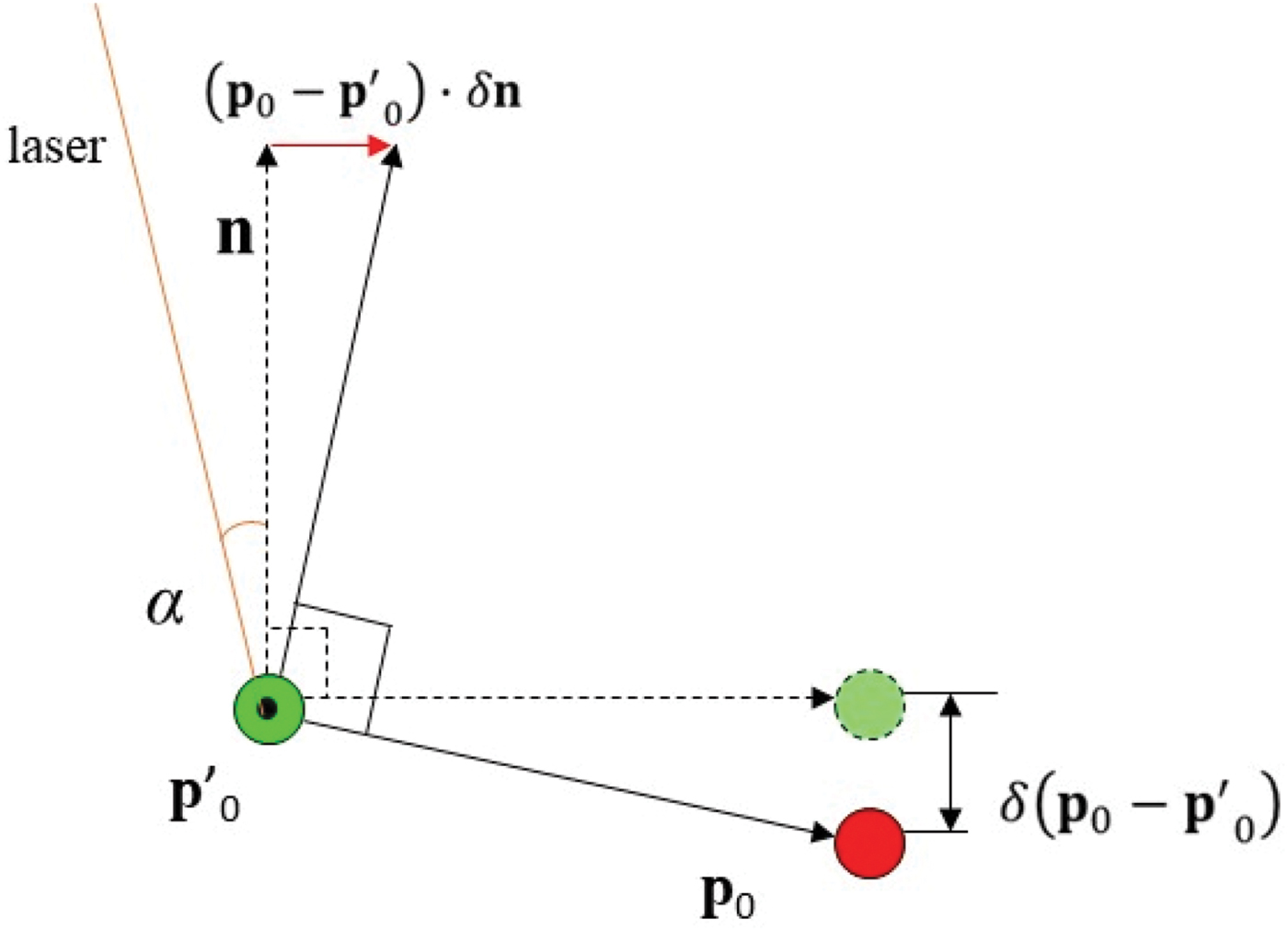
Figure 4. Errors in normal vector n caused by LADAR measurement uncertainty.
Recall that Equation (18) shows that LADAR errors in points
 ${\bf{p}}_{0}$
and
${\bf{p}}_{0}$
and
 ${\bf{p}}'_{0}$
result in angular errors in n, in the direction of
${\bf{p}}'_{0}$
result in angular errors in n, in the direction of
 $\lpar {\bf{p}}_{0}-{\bf{p}}'_{0} \rpar \times {\bf{n}}$
. Let e
n
be the magnitude of
$\lpar {\bf{p}}_{0}-{\bf{p}}'_{0} \rpar \times {\bf{n}}$
. Let e
n
be the magnitude of
 $\Delta {\bf{\Omega}}$
projected onto the direction of
$\Delta {\bf{\Omega}}$
projected onto the direction of
 $\lpar {\bf{p}}_{0}-{\bf{p}}'_{0} \rpar \times {\bf{n}}$
, i.e.,
$\lpar {\bf{p}}_{0}-{\bf{p}}'_{0} \rpar \times {\bf{n}}$
, i.e.,
 $$e_{n}\vert \lpar {\bf{p}}_{0}-{\bf{p}}'_{0} \rpar \times {\bf{n}} \vert =\vert \delta \lpar {\bf{p}}_{0}-{\bf{p}}'_{0} \rpar \vert $$
Hence,
 $$e_{n}={\vert \delta \lpar {\bf{p}}_{0}-{\bf{p}}'_{0} \rpar \vert \over \vert \lpar {\bf{p}}_{0}-{\bf{p}}'_{0} \rpar \vert }$$
Taking into consideration Equations (12) and (13), the angular error of the normal vector can be directly related to the LADAR ranging error σ via:
 $$e_{n}={1\over \vert \lpar {\bf{p}}_{0}-{\bf{p}}'_{0} \rpar \vert }\left(\sqrt {{1\over L}\sigma^{2}+{1\over L'}\sigma^{2}} \right)$$
To further simplify this approach, assume that
 $\Delta \Omega$
has the same magnitude of error in all dimensions, each of which can be over-bounded with e
n
. The three DOF error magnitude is thus estimated with
$\Delta \Omega$
has the same magnitude of error in all dimensions, each of which can be over-bounded with e
n
. The three DOF error magnitude is thus estimated with
 $\sqrt 3 e_{n}$
.
$\sqrt 3 e_{n}$
.
The relationship between the distance error and σ can also be defined. Recall that the distance between the LADAR and the surface can be computed using all L points on {Line1}:
 $$\rho ={1\over L}\sum_{l=1}^L {{\bf{\rrho}}_{l}} \cdot{\bf{n}}=\bar{\bf{\rrho}}\cdot {\bf{n}}$$
The error in the distance can then be found as follows:
 $$\delta \rho ={1\over L}\sum_{l=1}^L {{\delta {\bf{\rrho }}}_{l}} \cdot {\bf{n}}+\bar{\bf{\rrho} }\cdot \delta {\bf{n}}$$
As shown in Figure 4, α is the angle of incidence of the laser beam at
 ${\bf{p}}'_{0}$
, which can be computed using an estimated n. As a result, the angle between the laser beam at
${\bf{p}}'_{0}$
, which can be computed using an estimated n. As a result, the angle between the laser beam at
 ${\bf{p}}'_{0}$
and vector
${\bf{p}}'_{0}$
and vector
 $\delta {\bf{n}}$
is
$\delta {\bf{n}}$
is
 ${\pi \over 2}-\alpha $
, and
${\pi \over 2}-\alpha $
, and
 $\bar{\bf{\rrho} }\cdot \delta {\bf{n}}=\vert \bar{\bf{\rrho}}\vert \cdot \vert \delta {\bf{n}}\vert \cdot \sin(\alpha)$
. Since all the scan points are assumed to be independent from each other, the variance of distance can be estimated by:
$\bar{\bf{\rrho} }\cdot \delta {\bf{n}}=\vert \bar{\bf{\rrho}}\vert \cdot \vert \delta {\bf{n}}\vert \cdot \sin(\alpha)$
. Since all the scan points are assumed to be independent from each other, the variance of distance can be estimated by:
 $$\sigma_{\rho }^{2}={1\over L}\sigma^{2}+\left[ {\vert \bar{\bf{\rrho} }\vert \over \vert \lpar {\bf{p}}_{0}-{\bf{p}}'_{0} \rpar \vert } \right]^{2}\left( {{1\over L}\sigma^{2} }+{{1\over L'}\sigma^{2}} \right)\lpar \sin \alpha \rpar ^{2}$$
Equations (25) and (28) show that the uncertainties in normal vectors and the distances are dependent on the LADAR ranging noise, the number of points on both scans, and the separation between the two scan lines. Obviously, a smaller σ and a larger number of scan points on both lines are desirable. When the two line segments are almost in parallel and further away from each other, a greater value of
 $|({\bf{p}}_{0}-{\bf{p}}'_{0})|$
can be observed, and the estimates are more accurate.
$|({\bf{p}}_{0}-{\bf{p}}'_{0})|$
can be observed, and the estimates are more accurate.
Further, when the laser ray is nearly parallel to n, which happens often when a horizontal LADAR scans vertical objects, α approaches zero. In this case, the error modelled in Equation (28) is dominated by a single term
 ${{1\over L}\sigma^{2}}$
. By contrast, in some cases, the ray is almost in parallel to the surface, for example, when a nearly horizontal LADAR scans the floor or the ceiling. The angle of incidence would be close to 90°, and there will be a greater amount of uncertainty in the planar distance estimates in that case. The LADAR is not expected to scan any plane with a 90° angle of incidence.
${{1\over L}\sigma^{2}}$
. By contrast, in some cases, the ray is almost in parallel to the surface, for example, when a nearly horizontal LADAR scans the floor or the ceiling. The angle of incidence would be close to 90°, and there will be a greater amount of uncertainty in the planar distance estimates in that case. The LADAR is not expected to scan any plane with a 90° angle of incidence.
3.3. Bias Induced by a Moving Object
The motion of a moving planar surface can be decomposed into two components in the LADAR body frame, a translational component and a rotational one. Here, “translational motion” refers to the situation where the distance ρ of a plane changes while the normal vector n stays constant. Similarly, “rotational motion” defines the movement of a plane that has a constant ρ and a varying n.
Suppose that only a single surface k out of a total of M surfaces is moving. In that case, the translational motion component pollutes the measurement Y with a bias ρ b .
 $${\bf{Y}}=\lsqb \lpar \rho_{i1}-\rho_{j1} \rpar ,\ldots\lpar \rho_{ik}-\rho_{jk} \rpar +\rho_{b},\ldots ,\lpar \rho_{iM}-\rho_{jM} \rpar \rsqb ^{T}$$
Matrices
 ${\bf{H}}$
and
${\bf{H}}$
and
 ${\bf{H}}_{\Omega}$
remain the same since the normal vector of k has not changed. The k
th row of the solution Equation (2) is consequently changed into
${\bf{H}}_{\Omega}$
remain the same since the normal vector of k has not changed. The k
th row of the solution Equation (2) is consequently changed into
 $${\bf{n}}_{k}^{T}\cdot \Delta {\bf{R}}=\lpar \rho_{ik}-\rho_{jk} \rpar +\rho_{b}$$
In the meanwhile, the range bias does not affect the rotation solution of Equation (7), since the normal vectors are unchanged due to a range bias.
On the other hand, a pure rotation of the k th surface does not affect the Y matrix, but changes the k th row of H:
 $${\bf{H}}_{{\Omega }}=\lsqb {\bf{n}}_{1}^{T},\ldots \tilde{\bf{n}}_{k}^{T},\ldots {\bf{n}}_{M}^{T} \rsqb ^{T}$$
where
 $\tilde{\bf{n}}_{k}^{T}$
reflects a rotation of
$\tilde{\bf{n}}_{k}^{T}$
reflects a rotation of
 ${\bf{n}}_{k}^{T}$
, which can be linearized using
${\bf{n}}_{k}^{T}$
, which can be linearized using
 $$\tilde{\bf{n}}_{k}^{T}={\bf{n}}_{k}^{T}+\Delta {\bf{\Omega}}\times {\bf{n}}_{k}^{T}={\bf{n}}_{k}^{T}+{\bf{n}}_{b}^{T}$$
where
 ${\bf{n}}_{b}^{T}$
is the bias on the normal vector. As a result, the k
th row of solution Equation (2) becomes:
${\bf{n}}_{b}^{T}$
is the bias on the normal vector. As a result, the k
th row of solution Equation (2) becomes:
 $${\bf{n}}_{k}^{T}\cdot \Delta {\bf{R}}=(\rho_{ik}-\rho_{jk})-{\bf{n}}_{b}^{T}\cdot \Delta {\bf{R}}$$
Obviously, the rotational motion may be observable in both displacement and rotation solutions.
3.4. Detecting the Translational Motion
When only considering the translational motion, the noise in H is negligible. Thus,
 $${\bf{H}}=\lsqb {\bf{n}}_{1}^{T},\ldots {\bf{n}}_{M}^{T} \rsqb ^{T}$$
and errors are observed on Y only.
 $$\eqalign{\tilde{\bf{Y}}=& \lsqb \lpar \rho_{i1}-\rho_{j1} \rpar +\delta \lpar \rho_{i1}-\rho_{j1} \rpar ,\ldots \lpar \rho_{ik}-\rho_{jk} \rpar +\rho_{b}+\delta \lpar \rho_{ik}-\rho_{jk} \rpar ,\ldots ,\lpar \rho_{iM}-\rho_{jM} \rpar \cr & + \delta \lpar \rho_{iM}-\rho_{jM} \rpar \rsqb ^{T}}$$
A residual-based procedure can be implemented for outlier detection.
-
1. Perform a QR decomposition of
$\bf{H}:[\bf{Q},\bf{R}]=qr({\bf{H}})$
. -
2. Define matrix
${\bf{Q}}_{{\bf{p}}}$
based on the lower part of
${\bf{Q}}^{T}: {\bf{Q}}_{{\bf{p}}}={\bf{Q}}^{T}(4{:}\ M,1{:}\ M)$
. Obviously for bias detection, the total number of surfaces has to be at least four. -
3. Compute the residuals in parity space using
(36)which include noise and bias terms, since
$${\bf{p}}={\bf{Q}}_{{\bf{p}}}\tilde{\bf{Y}}$$
${\bf{Q}}_{{\bf{p}}}\tilde{\bf{Y}}={\bf{Q}}_{{\bf{p}}}{\bf{\rvarepsilon}}$
, where
${\bf{\rvarepsilon }}=[ \delta ( \rho_{i1}-\rho_{j1} ),\ldots\break \rho_{b}+\delta ( \rho_{ik}-\rho_{jk} ),\ldots ,\delta ( \rho_{iM}-\rho _{jM} ) ]^{T}$
.
-
4. Since noise from all individual points are assumed to be independent, the covariance matrix can be defined as
(37)which can be estimated based on Equation (24).
$${\bi{COV}}_{{\bf{Y}}}=\bi{diag}\lsqb \sigma_{\rho_{i1}}^{2}+\sigma_{\rho_{j1}}^{2},\ldots\sigma_{\rho_{iM}}^{2}+\sigma_{\rho_{jM}}^{2} \rsqb $$
-
5. The covariance of the residual can be estimated with
(38)
$${\bi{COV}}_{{\bf{p}}}={\bf{Q}}_{{\bf{p}}}\cdot \bi{COV}_{{\bf{Y}}}\cdot {\bf{Q}}_{{\bf{p}}}^{{\bf{T}}}$$
-
6. A threshold for judging if object l is in motion can thus be defined with
(39)where γ will be chosen for a required misdetection probability. A corresponding Minimum Detectable Bias (MDB) for object l is then estimated with
$$C_{l}=\gamma \sqrt{{\bi{COV}}_{\bf{p}}(l,l)}$$
(40)
$$MDB_{l}=\beta \sqrt{{\bi{COV}}_{{\bf{p}}}(l,l)}$$


In a practical implementation, γ and β are both defined a priori, for example, based on the assumption of Gaussian distribution. This assumption, however, will be verified using simulated data.
3.5. Detecting the Rotational Motion
Since it is likely for a moving object to have both translational and rotational motion, one may argue that outlier detection can solely rely on the detection of translational motion. However, it will be shown in this section that the detection algorithm for rotation tends to be more sensitive and can flag a moving object more reliably.
Unlike the detection of translational bias, rotational outlier detection is based on the orientation solution in Equation (7). In this case, the random errors in the normal vectors can no longer be ignored.
 $$\Delta \tilde{\bf{n}}=\left[ \matrix {{{(\hat{\bf{C}}}_{j}^{i})}_{0}\cdot \lpar {\bf{n}}_{i1}+\delta {\bf{n}}_{i1} \rpar -\lpar {\bf{n}}_{j1}+\delta {\bf{n}}_{j1} \rpar \cr \ldots \cr {{(\hat{\bf{C}}}_{j}^{i})}_{0}\cdot \lpar {\bf{n}}_{ik}+\delta {\bf{n}}_{ik}+{\bf{n}}_{b} \rpar -\lpar {\bf{n}}_{jk}+\delta {\bf{n}}_{jk} \rpar \cr \ldots \cr {{(\hat{\bf{C}}}_{j}^{i})}_{0}\cdot \lpar {\bf{n}}_{iM}+\delta {\bf{n}}_{iM} \rpar -\lpar {\bf{n}}_{jM}+\delta {\bf{n}}_{jM} \rpar } \right]$$
With the
 ${\bf{H}}_{\Omega}$
matrix equal to:
${\bf{H}}_{\Omega}$
matrix equal to:
 $${\bf{H}}_{\Omega}=\left[ \matrix{\lpar {\bf{n}}_{i1} \rpar \times \cr \ldots \cr \lpar {\bf{n}}_{ik}+{\bf{n}}_{b} \rpar \times \cr \ldots \cr \lpar {\bf{n}}_{iM} \rpar \times}\right]$$
With random errors and bias,
 $$\Delta \tilde{\bf{n}}={\bf{H}}_{\Omega}\cdot \Delta {\bf{\Omega}}$$
The 3M by 3M covariance matrix of
 $\Delta {\bf{n}}$
is estimated based on Equation (25). Since
$\Delta {\bf{n}}$
is estimated based on Equation (25). Since
 $\Delta\bf{n}$
is affected by noise from both frame i and j:
$\Delta\bf{n}$
is affected by noise from both frame i and j:
 $${\bi{COV}}_{{\bf{n}}}=\bi{diag}\lsqb 2e_{n,1}^{2},2e_{n,1}^{2},2e_{n,1}^{2},\ldots 2e_{n,M}^{2},2e_{n,M}^{2},2e_{n,M}^{2} \rsqb $$
The residual-based bias detection procedure introduced in Section 3.4 can now be repeated using
 ${\bf{H}}_{{\Omega }}$
and
${\bf{H}}_{{\Omega }}$
and
 ${\bi{COV}}_{{\bf{n}}}$
. The complexity of the proposed navigation and outlier detection algorithms is thus O(M), and M is the number of features in each epoch.
${\bi{COV}}_{{\bf{n}}}$
. The complexity of the proposed navigation and outlier detection algorithms is thus O(M), and M is the number of features in each epoch.
Every planar normal vector is a 3D vector that limits the solution by two DOF. As a result,
 ${\bf{H}}_{{\Omega }}$
has 3M rows, among which 2M rows are expected to be independent. Thus, the parity space has (3M-3) dimensions. In theory, a minimum of two non-parallel planar surfaces is sufficient for rotation solution, and it can already produce a scalar residual.
${\bf{H}}_{{\Omega }}$
has 3M rows, among which 2M rows are expected to be independent. Thus, the parity space has (3M-3) dimensions. In theory, a minimum of two non-parallel planar surfaces is sufficient for rotation solution, and it can already produce a scalar residual.
4. SIMULATION AND FIELD TESTING RESULTS
4.1. Software Simulation
In a software-based simulation, a 2D LADAR is created with an angular range of 180° and
 $0{\cdot}5^{\circ}$
resolution. This LADAR scans at 1 Hz, with a ranging accuracy of 0·01 m (1σ ). No planar surface texture has been simulated, therefore,
$0{\cdot}5^{\circ}$
resolution. This LADAR scans at 1 Hz, with a ranging accuracy of 0·01 m (1σ ). No planar surface texture has been simulated, therefore,
 $\sigma =0{\cdot}01\,\hbox{m}$
.
$\sigma =0{\cdot}01\,\hbox{m}$
.
The LADAR scans four surfaces at multiple elevation angles, as shown in Figure 5. The scans at 0° and 10° are used to derive planar surfaces. Only two epochs are simulated; at t=0 s the LADAR is at the origin of the local East North Up (ENU) frame, and at t=1 s it steps onto location
 $[0{\cdot}4\ 0{\cdot}6\ 0{\cdot}0]$
m. It is assumed that all the scans have been compensated by an IMU, and thus no IMU errors are simulated. On average, there are 50 points on each scan line.
$[0{\cdot}4\ 0{\cdot}6\ 0{\cdot}0]$
m. It is assumed that all the scans have been compensated by an IMU, and thus no IMU errors are simulated. On average, there are 50 points on each scan line.

Figure 5. Simulated planar surfaces.
The uncertainty of normal vector errors and distance errors can now be estimated. As previously mentioned, the standard deviation of
 $\vert \delta {\bf{n}}\vert $
can be approximated with
$\vert \delta {\bf{n}}\vert $
can be approximated with
 $\sqrt 3 e_{n}$
, which is computed using Equation (25). Similarly, σρ is estimated using Equation (28). They are compared against the standard deviation from the Monte Carlo simulation, listed in Table 1. The estimate closely predicts the standard deviation values, except for a pessimistic estimate of the first planar surface. Since the simplified model is expected to be conservative, it is not surprising to observe this deviation.
$\sqrt 3 e_{n}$
, which is computed using Equation (25). Similarly, σρ is estimated using Equation (28). They are compared against the standard deviation from the Monte Carlo simulation, listed in Table 1. The estimate closely predicts the standard deviation values, except for a pessimistic estimate of the first planar surface. Since the simplified model is expected to be conservative, it is not surprising to observe this deviation.
Table 1. Estimated Sigma Value and Monte Carlo Standard Deviation of errors in normal vector and distance.

Next, a moving object is simulated with pure translational motion on one of the four surfaces. The surface is moved away from the LADAR by 0·1 m at epoch 1, which represents a 0·1 m/s linear velocity. With only four surfaces in the FOV, the residual space for translational bias detection collapses into a scalar value. It is also simulated in a 100-run Monte Carlo simulation. Figure 6 compares the estimated Probability Density Function (PDF) of the residual value with and without the bias. The bias is clearly visible in the residual space, as there is no overlap between both PDFs. Obviously it is unlikely to directly observe misdetections or false alarms with only 100 runs when their probabilities are so small. However, 100 runs are sufficient to test the residuals against known statistical distributions. In this case, the residuals of both simulations are found to follow a Gaussian distribution (χ2 goodness-of-fit test, 5%). A detection threshold of 0·03 m is computed from Equation (35) using
 $\gamma =4{\cdot}4$
, which corresponds to a 10−5 misdetection probability for a single residual.
$\gamma =4{\cdot}4$
, which corresponds to a 10−5 misdetection probability for a single residual.

Figure 6. Residuals with and without bias from the displacement solution.
The third experiment tests the bias detection for a rotating object. This time, the LADAR does not step to a different location. Instead, the heading is turned by 5°. The moving surface keeps a constant distance to the LADAR, but is rotated by
 $5{\cdot}7^{\circ}$
(0·1 rad/s). As mentioned in Section 3, with M=4 planar surfaces, there are 12 linear equations. The residual space contains up to nine dimensions. One of the dimensions is chosen to illustrate the distribution of the residuals. The PDFs of the residuals with and without a rotating object are shown in Figure 7. Both follow a Gaussian distribution (χ2 goodness-of-fit test, 5%). The detection threshold (10−5 misdetection probability) is 0·013 rad, which again detects all the biased cases without false alarms in these Monte Carlo runs.
$5{\cdot}7^{\circ}$
(0·1 rad/s). As mentioned in Section 3, with M=4 planar surfaces, there are 12 linear equations. The residual space contains up to nine dimensions. One of the dimensions is chosen to illustrate the distribution of the residuals. The PDFs of the residuals with and without a rotating object are shown in Figure 7. Both follow a Gaussian distribution (χ2 goodness-of-fit test, 5%). The detection threshold (10−5 misdetection probability) is 0·013 rad, which again detects all the biased cases without false alarms in these Monte Carlo runs.

Figure 7. Residual with and without bias from the rotation solution.
4.2. LADAR-Only Field Test Results
The objective of the preliminary test was to verify the detection algorithm using real LADAR data in a well-controlled environment. Two HOKUYO URG 04LX LADARs were used, which are relatively low-cost indoor-only units, capable of scanning 240° in angular range and 60 to 4095 mm in distance, at scanning rates up to 10 Hz. These LADARs, however, may not support outdoor applications. Both units are collocated and set with a constant offset in elevation angle. Without using an IMU, both units are kept stationary throughout the experiment.
Both LADARs are installed on a rigid platform, and placed near a selected corner of an office. There are several planar surfaces in the LADAR FOV, including the walls, the ceiling and the door, all of which are relatively flat and smooth. In this environment, it is estimated that
 $\sigma \approx 0{\cdot}015\,\hbox{m}$
. The office door is opened and closed several times to create both translational motion and rotation of a planar surface.
$\sigma \approx 0{\cdot}015\,\hbox{m}$
. The office door is opened and closed several times to create both translational motion and rotation of a planar surface.
The LADAR displacement and rotation are measured between two epochs, i and j. In this stationary experiment, epoch i is always the first measurement epoch of the data set, whereas a second epoch j can be selected from any of the other 183 scans taken in approximately 50 seconds. Thus, different levels of door motion between i and j can be observed with a single dataset.
The door motion between epochs i and j is illustrated with the angle, of which zero means closed and 90° means fully open. As shown in the lower part of Figure 8, the angle changes between 0 and 90° periodically during the 50 s window. Without removing the moving surface from the solution, the forward(X)-right(Y)-down(Z) displacement errors change accordingly to the door motion, as shown in Figure 8. Among the three axes, error in the right direction has the greatest change. This is most likely due to the fact that the LADARs are sideways to the door. The rotational errors can be seen in Figure 9, where X-Y-Z represent roll, pitch and yaw respectively. Similarly, the moving door does not directly change the pitch angle estimates, since it is perpendicular to the ground. However, the effect on yaw angle is substantial.

Figure 8. Displacement error due to a moving door in 3D LADAR odometry.

Figure 9. Rotation error due to a moving door in 3D LADAR odometry.
Next, the moving door is detected in the parity space, of displacement and rotation solutions respectively. As shown in Figure 10, the residuals from the displacement solution clearly reflect the pattern of the door angle. It is compared against a detection threshold in the upper graph of Figure 10. It has been calculated that the MDB of the door angle is approximately 40°, which indicates that the motion of the door can be reliably detected when it opens for more than 40° between the two epochs in the displacement solution. The lower graph of Figure 10 shows the residuals and threshold from the rotation solution. The threshold appears much lower in this graph than in the position solution. This indicates that the detection algorithm is much more sensitive in the rotation solution. Indeed, the estimated MDB in this case is approximately 8°, which is a lot lower than the MDB in a displacement solution.

Figure 10. Residuals in displacement and rotation solution in 3D LADAR odometry.
4.3. Preliminary Field Test Results
A practical LADAR navigation system for a small UAV would include compact LADAR and IMU sensors. It requires precise alignment and synchronisation between LADAR and IMU.
The LADAR/IMU data collection system designed for this test consists of a Xsens MTi-G700 GPS/IMU unit, a Hokuyo UTM30LX LADAR, a Hokuyo UST20LX LADAR and a Raspberry Pi B computer. All sensors have been mounted on a rigid structure. As shown in Figure 11, the pitch angles of both LADARs differ by approximately 30°. The range is specified as 30 m for the Hokuyo UTM30L, and 20 m for the Hokuyo UST20LX. Both LADARs are capable of indoor or outdoor use. LADAR scans and Xsens raw IMU messages are synchronised with the on board clock of the Raspberry Pi computer. The entire system is powered with a single three-cell LiPo battery, which make it a standalone sensor suite that can be installed on small UAVs.

Figure 11. Hokuyo lasers and IMU (LADAR1 on the bottom and LADAR2 on the top).
This sensor suite has been used to collect data in cluttered indoor spaces, such as the hallway shown in Figure 12. 1 Hz LADAR data and 100 Hz IMU messages are integrated in a post-processing EKF. The state space of this EKF includes position, orientation and velocity, as well as bias and scale factor states for gyroscopes and accelerometers. Displacement and rotation solutions from Equations (2) and (7) respectively are used to update the velocity and orientation states.

Figure 12. A narrow hallway with uneven surfaces for the field test.
Over 500 s of data collection, the sensor suite emulates a small UAV hovering in the hallway while moving objects were intentionally introduced. The system was slightly tilted with −10° pitch, which helps both LADARs to measure the floor. The number of planar features extracted at each epoch ranges from four to nine, with an average of six. The EKF used the first 40 s for zero velocity update. After that, the sensor suite was still held stationary to ensure the repeatability of the experiment, although the navigation solution runs as if it is freely moving. In the first 300 s, a door was opened and closed 15 times. It was followed by an object (a 60 cm by 90 cm board) approaching and departing from the sensor suite ten times, as shown in Figure 13. The moving objects would be detected in either displacement or rotation solutions, and whenever possible, would be isolated. Detection thresholds corresponding to a 5% false alarm rate are used.

Figure 13. Angle of an opening door and distance to a moving object in the field test.
There are additional challenges besides the moving objects. Unlike the controlled environment used in Section 4.2, surfaces of the floor, wall and other objects are not entirely flat or smooth. Consequently, the line segments in both LADAR scans may not be completely coplanar on some of these surfaces, which essentially results in the fictitious planar features. These features are not always repeated from epoch to epoch, due to randomness in line extraction. Unfortunately, they will be perceived as motion of planar surfaces, which cause small biases in displacement and rotation estimation. These biases can be reliably flagged as outliers, and will not directly jeopardize the integrity of the navigation solution. However, they do cause more updates to be abandoned, and thus further reduce the availability of corrections.
Since both moving objects and fictitious planes can be detected, the solution from the EKF is still mostly consistent. As shown in Figure 14, with the exception of a few points, the velocity errors are within the 3-sigma bounds in all three directions. The horizontal position error, with respect to a known location as truth reference after 500 s is approximately 10 m, which exhibits expected performance for an odometry system. The standard errors of velocity are
 $[0{\cdot}058\ 0{\cdot}026\ 0{\cdot}032]$
m/s in all three dimensions, and [3 2 5] mrad in roll, pitch and heading.
$[0{\cdot}058\ 0{\cdot}026\ 0{\cdot}032]$
m/s in all three dimensions, and [3 2 5] mrad in roll, pitch and heading.

Figure 14. Velocity error from EKF (solid), bounded by 3-sigma curves (dashed). The filter was initialised in the first 40 seconds (not shown).
As mentioned, Monte Carlo Localisation is one of the commonly used alternatives to LADAR odometry. In this work, a MATLAB® implementation of the Adaptive Monte Carlo Localization (AMCL) algorithm (Fox, Reference Fox2003) has been used. The a priori map required by the AMCL can be an occupancy grid map estimated with the initial scans of a local area. A predicted motion model from the IMU is coupled with 2D scans from LADAR1, as shown in Figure 11, to form a solution of 2D position and heading with respect to the initial map.
For a fair comparison against the LADAR odometry, North and East velocities have been derived from the AMCL position estimates. The standard errors of velocity and heading are [0·034 m/s, 0·027 m/s and 75 mrad]. On average, velocity errors have similar levels of magnitude to those from the proposed six DOF solution, although they exhibit quite different patterns, as illustrated in Figure 15. Without an explicit outlier detection step, AMCL is not always robust against moving objects, which results in increased errors in velocity and heading. However, AMCL could potentially make use of all available scan points. Since only a small portion of all the scan points (no greater than 10% at each epoch) is affected by moving objects, the estimated position or velocity is still expected to be less noisy in general.

Figure 15. Velocity error from map-based 2D localisation. Since the estimated uncertainty is overly conservative, 3-sigma curves are not included in the figure. Increased error magnitude is due to moving objects.
5. DISCUSSIONS AND SUMMARY
The six DOF odometry solution discussed in this work is capable of estimating motion in consecutive epochs by comparing the observations of planar features. It does not attempt to locate any features as landmarks, and neither does it use a map of any kind. As a result, the complexity is only proportional to the number of features in the current FOV. Since it only needs a few features in the FOV at each epoch, the computational cost is well under control. Unlike the SLAM solutions that would have difficulties handling a large-sized map, LADAR odometry is a scalable solution. On the other hand, it cannot benefit from pose corrections at loop closure events as SLAM solutions do.
Velocity and orientation estimates are critical to autonomous control and guidance of small UAVs. Horizontal velocity and heading would be available from a regular three DOF solution, such as the MCL. Vertical velocity, roll and pitch angles only become available in a six DOF solution, which would help the UAV accurately sense the attitude and maintain stability in the air. The proposed approach enables the six DOF solution by using two concurrent 2D LADAR scans, instead of a complete 3D point cloud.
To form a six DOF solution, three non-parallel planar features are needed in the FOV. Unlike grid-map-based solutions, these features are not always available in an arbitrary environment. Luckily, it would not be difficult to find them in an urban or indoor scenario, such as two walls at a corner and the floor. However, in the displacement solution, at least one additional surface is needed to form an over-determined solution for outlier detection. By contrast, a minimum of two non-parallel planar surfaces is sufficient for outlier detection in the rotation solution. The rotation solution is very sensitive to the rotational motion of a moving object, but cannot observe outliers caused by pure translational motion. For example, a moving person or vehicle directly facing the LADAR can only be detected in the displacement solution. For a robust solution, it is recommended that outlier detection be performed simultaneously in both solutions.
Outlier detection is a first step toward a navigation solution with protected integrity. However, since it requires four features in the FOV, the availability of the solution may potentially be affected. Furthermore, the estimated velocity in this approach appears to have more noise than that from the grid-map-based odometry. In future work, different aspects of navigation performance, including integrity, accuracy, and availability will have to be evaluated in a variety of indoor and urban scenarios.
FINANCIAL SUPPORT
This work was partly supported by the Air Force Office of Scientific Research, grant FA9550-07-1-0383.


