


1. INTRODUCTION
Precise relative positioning based on Global Navigation Satellite Systems (GNSS) is the key to numerous space applications such as satellite rendezvous, formation flying and spacecraft collision avoidance. Current methods used to evaluate inter-satellite separation rely on Global Positioning System (GPS) code and carrier phase measurements [Reference Kroes and Montenbruck1, Reference Kroes2]. The expected level of precision when using pseudo-ranges only is a few metres when no corrections are applied. If the phases of the carrier are also used, the precision of relative positioning estimates can go down to a few millimetres once carrier phase ambiguities are resolved. However, the task is often daunting and is still the topic of continuing research [Reference Psiaki and Mohiuddin3, Reference Mohiuddin and Psiaki15].
In this study, an easier-to-implement method – based on single-frequency pseudorange measurements only – was developed. It allows for a decimetre-level accuracy. In addition, the utilization of single-frequency receivers can afford a substantial reduction in the overall cost of space missions, notably those featuring micro-satellites. This method was evaluated using raw empirical data from the Gravity Recovery and Climate Experiment (GRACE) mission. It is important to note that data were not processed within the framework of this article: no filtering algorithm or corrections were applied.
The GRACE mission features two identical satellites in a leader-follower formation (GRACE A and GRACE B) orbiting the Earth on the same orbital plane. Their initial altitude above the Earth surface was close to 500 km. Due to atmospheric drag, it will decrease to about 300 km towards the end of the mission. The mean inter-satellite separation varies between 170 and 270 km. Originally funded for a five-year period (2002–2007), the mission has been further extended to 2009. As the orbit decay has been slower than initially thought and the satellites' current fuel supply is expected to last another four years at the very least, the mission is likely to continue past 2012.
This article is organized as follows. In Section 2, data used throughout this study are described:
• Pseudoranges between the GRACE spacecraft and all of the GPS satellites in sight.
• Ephemeris data characterizing the orbit and clock of all of the relevant GPS satellites.
• GRACE inter-satellite separation collected by the K-Band Ranging (KBR) system.
• GRACE navigation data (GNV), which include post-processed position and velocity solutions.
Section 3 focuses on the performances of two relative positioning algorithms. The first one is based on the difference between two absolute position vectors. This method is frequently used and numerous techniques have been designed to address its major shortcoming, namely taking into account twice the errors common to both of the satellites (such as atmospheric propagation delays or ephemeris uncertainty) before their expected mutual cancellation in the differencing process [Reference Misra and Enge4].
The second algorithm was initially conceived for aircraft collision avoidance [Reference Rudel and Baldwin5]. Through this research, it has been validated for spaceborne applications for the first time. As it solves directly for the relative position vector, errors affecting simultaneously the two satellites are cancelled at the source. A large-scale analysis undertaken on behalf of the Galileo Future Applications project (GEO-6) showed that the relative positioning error could be reduced by up to two orders of magnitude when using the ‘direct’ method.
2. DATA ACQUISITION
Actual data from a formation of satellites equipped with GPS receivers were essential to verify and validate the positioning algorithms. Data collected by the GRACE satellites enabled such an endeavour. Two sets of data were needed to calculate the relative position between GRACE A and GRACE B:
• Pseudoranges between each satellite and all of the GPS satellites it has in view.
• Ephemeris data characterizing each of these GPS satellites.
In addition, the inter-satellite separation derived from the K-Band Ranging system measurements was used as a ‘true’ reference against which the calculated distances were compared.
2.1. GRACE Observation Data
GRACE A and GRACE B observation data can be found on the mission's official website maintained by the Jet Propulsion Laboratory.Footnote 1 Observation files contain pseudoranges and phase measurements for each of the GRACE satellites. Data used in this study were recorded on four different three-day-long periods. As the sampling frequency was equal to 0·1 Hz, the expected total number of measurements amounted to 25 920 for each period.
GPS satellites transmit data on two L-band frequencies: L 1=1575·42 MHz and L 2=1227·6 MHz. Pseudo-random noise (PRN) ranging codes in use include the coarse acquisition (C/A) code and the precision (P) code. C/A code is available on the L 1 frequency only whereas the P-code is available on both L 1 and L 2.
Using the C/A code and the P-code on both L 1 and L 2, pseudoranges between GRACE satellites and each of the GPS satellites they respectively had in view (between 1 and 10 for GRACE A, 2 and 10 for GRACE B) were extracted and stored for subsequent calculations. The graphs presented in this article were based on the P 1-code for the January 1st–3rd, 2007 period unless otherwise specified.
2.2. GPS Data
Global GPS Navigation files were obtained from the National Geodetic Survey websiteFootnote 2. They contain ephemeris data for each of the GPS satellites. GPS satellite numbers (also known as PRN number after the unique pseudo-random noise associated with each satellite) range from 1 to 31. However, on limited occurrences just 30 GPS satellites were in view as some of the satellites could not be seen – by either GRACE A or GRACE B – during the 72-hour measurement periods under consideration or were not operating at that time. A description of the GPS constellation for each epoch can be found on the U.S. Coast Guard website.Footnote 3
For each of the GPS satellites, 19 parameters characterizing their respective orbit and clock were extracted. Using the broadcast ephemeris data, GPS satellites' coordinates were calculated in the WGS-84 (World Geodetic System) Earth-Centred Earth-Fixed (ECEF) reference frame. To this end, the algorithm found in Reference [6] was modified as it superfluously introduces the functions cos−1 and tan−1, the use of which may be critical for values at the boundary of the definition domain. A variation on the derivations of the second harmonic perturbations (corrections made to orbit parameters such as the argument of latitude, radius and inclination) that does not resort to reciprocal trigonometric functions is presented in the Appendix.
2.3. GRACE KBR and GNV data
K-Band Ranging (KBR) data files provide biased ranges between GRACE A and GRACE B along with the light time and antenna offset corrections that must be added. True ranges were obtained by calculating the bias as many times as needed over the 72-hour time periods (typically between once and thrice). GRACE navigation (GNV) data, which contain the post-processed positions and velocities for both satellites were used to estimate the bias. The true ranges thus computed served as a benchmark against which the distances generated by the different relative positioning algorithms were compared. As the typical sampling rate was 0·2 Hz (twice the GPS data rate), every other measurement was discarded to ensure a perfect correspondence between the data.
3. KINEMATIC STUDY
Two different approaches were used to evaluate the relative position between the GRACE satellites. The first method consists of solving the GPS absolute positioning equations for each of the satellites and differencing the position vectors thus obtained. The algorithm developed by Milliken and Zoller in 1978 offers an elegant solution to the absolute positioning problem. Its principle, detailed in Reference [Reference Milliken and Zoller7], is summarized in Section 3.1. The major drawback of this method is that errors common to both of the GRACE satellites such as ionospheric propagation delays, GPS satellite clock drifts or relativistic effects must be taken into account twice, even though they are expected to cancel out during the differentiation process. To remedy this issue, GPS relative positioning equations were formulated in Reference [Reference Rudel and Baldwin5]. They allow one to eliminate at the source errors that affect simultaneously two nearby spacecraft and to solve directly for the relative position vector. A detailed exposé of this method is given in Section 3.2.
Relative positions between GRACE A and GRACE B were computed and their norm was compared to the ‘true’ ranges derived from the KBR measurements. A significant increase in terms of accuracy was achieved when using the latter algorithm (see Section 3.3).
3.1. Absolute Positioning
Absolute positioning equations can be solved provided that a minimum of four GPS satellites are in view from the spacecraft under consideration.
Let A and S A, i respectively represent GRACE A and one of the n GPS satellites it has in view (i∊ℕn). rA and ri denote the position vectors of GRACE A and S A, i; rA, i, the vector from A to S A, i (see Figure 1). rA, i can be rewritten as:
In addition, rA, i is related to the broadcast pseudorange ρA, i as follows:
where e A stands for the range equivalent of GRACE A's clock offset and e A, i for the range equivalents of the GPS satellites' clock offsets.

By reorganizing terms, the absolute positioning equation is obtained:
The left-hand side of Equation (3) contains the unknown position vector rA and the associated error e A; the right-hand side of the equation, observable data.
The unit vector uA, i, also known as line-of-sight vector, must be estimated with an external device. For algorithmic purposes, an algebraic solution to the GPS equations found in Reference [Reference Bancroft8] was used to calculate an initial position estimate and hence an approximate value of the line-of-sight vector. Though the latter may be inaccurate, the iterative algorithm based on Equation (3) generally converges rapidly and stops whenever the distance between two consecutive position estimates does not exceed a fixed value set to 1 mm.

Figure 1. Absolute spatial configuration.
Similarly, let B and S B, j respectively represent GRACE B and one of the p GPS satellites it has in view (j∊ℕp). rB and rj denote the position vectors of GRACE B and SB, j respectively and rB, j, the vector from B to S B, j. e B stands for the range equivalent of GRACE B's clock offset and e B, j for the range equivalents of the GPS satellites' clock offsets. The absolute positioning equation for GRACE B is expressed as:
The ECEF coordinates of GRACE A and GRACE B, (x A, y A, z A) and (x B, y B, z B) respectively, were calculated every 10 s – as allowed by the measurement sampling rate – through Equations (3) and (4). They were used to plot GRACE satellites' common orbit as well as the satellites' altitude above the Earth's surface (see Figures 2 and 3).

Figure 2. 72-hour Earth coverage of GRACE satellites.

Figure 3. GRACE satellites' altitude above Earth's surface.
3.2. Relative Positioning
The distance between GRACE A and GRACE B can be derived by differencing the absolute position vectors of the two satellites; alternatively, it can be directly expressed as a result of the relative positioning equations.
Let A and B represent satellites GRACE A and GRACE B. S A, i and S B, j respectively denote the i th GPS satellite in view from A and the j th GPS satellite in view from B, where (i, j)∊ℕn×ℕp. The vectors from A to B, A to S A, i, B to S B, j and S A, i to S B, j are designated as rA, B, rA, i, rB, j and ri, j respectively (see Figure 4).

Figure 4. Relative spatial configuration.
Let uA, i and uB, j represent the unit vectors of lines (AS A, i) and (BS B, j) respectively. rA, i and rB, j can be rewritten as:
where rA, i=‖rA, i‖ and rB, j=‖rB, j‖
In addition, rA, i and rB, j are related to the broadcast pseudoranges ρA, i and ρB, j by the equations:
where e A and e B stand for the range equivalents of GRACE A and GRACE B clock offsets, e A, i and e B, j, the range equivalents of the GPS satellites' clock offsets.

By reorganizing terms, the relative positioning equation is obtained:
The left-hand side of Equation (7) contains the unknown position vector rA, B and the associated error e A−e B; the right-hand side of the equation represents observable data.
If the set of GPS satellites under consideration is further limited to those seen both by GRACE A and GRACE B (i=j=k), Equation (7) simplifies to:
This can be solved provided that the number of GPS satellites in common is greater than four (k⩾4).
Equation (8) can be written in a matrix form as: ![]() χ=
χ=![]() where
where ![]() is the k 2×4 weight matrix, χ the 4×1 relative position vector and
is the k 2×4 weight matrix, χ the 4×1 relative position vector and ![]() is the k×1 observable vector. The corresponding system of linear equations is generally overdetermined as k>4, but it can be solved using the pseudo-inverse matrix:
is the k×1 observable vector. The corresponding system of linear equations is generally overdetermined as k>4, but it can be solved using the pseudo-inverse matrix:
For the 72-hour period under consideration, the number of common satellites ranged between 0 and 9. Its variation over time, superimposed with the calculated distance between the GRACE satellites, is displayed in Figure 5. Close to 70% of the time, a minimum of six GPS satellites could be seen simultaneously by GRACE A and GRACE B, as illustrated by the histogram displayed on Figure 6.

Figure 5. Variation of the number of GPS satellites in common.

Figure 6. Distribution of the number of GPS satellites in common.
The variation of the Relative Geometric Dilution of Precision (RGDOP), which takes into account the configuration of the GPS satellites in common, was also investigated. Using the notations of Equation (9), the RGDOP can be determined by calculating the error covariance matrix as: ![]() =[
=[![]() t
t![]() ]−1.
]−1.
![]() is a symmetric matrix, the diagonal elements of which represent the variances on the relative position coordinates (x, y, z) and time offset t and the non-diagonal ones, the cross-correlation factors between those dimensions.
is a symmetric matrix, the diagonal elements of which represent the variances on the relative position coordinates (x, y, z) and time offset t and the non-diagonal ones, the cross-correlation factors between those dimensions.
![C \equals \left[ {\matrix{ {\sigma _{x}^{\setnum{2}} } \tab {\sigma _{xy} } \tab {\sigma _{xz} } \tab {\sigma _{xt} } \cr {\sigma _{xy} } \tab {\sigma _{y}^{\setnum{2}} } \tab {\sigma _{yz} } \tab {\sigma _{yt} } \cr {\sigma _{xz} } \tab {\sigma _{yz} } \tab {\sigma _{z}^{\setnum{2}} } \tab {\sigma _{zt} } \cr {\sigma _{xt} } \tab {\sigma _{yt} } \tab {\sigma _{zt} } \tab {\sigma _{t}^{\setnum{2}} } \cr} } \right]](https://static.cambridge.org/binary/version/id/urn:cambridge.org:id:binary:20151022094205295-0514:S0373463308005006_eqn10.gif?pub-status=live)
The Relative Geometric Dilution of Precision, represented in Figure 7, is defined as:
When the RGDOP is greater than 6, the occurrence can be referred to as an “outage”. As a general rule, the higher the number of common satellites, the lower and less dispersed the RGDOP tends to be. This is illustrated qualitatively in Figure 8 and quantitatively in Table 1, where the RGDOP mean and standard deviation (μRGDOP and σRGDOP respectively) are calculated as a function of the number of GPS satellites seen both by GRACE A and GRACE B.

Figure 7. Variations of the RGDOP (<40).

Figure 8. RGDOP dispersion (<40).
Table 1. RGDOP mean and standard deviation (m).

3.3. Error Analysis
The performances of the two positioning algorithms (the first one based on the difference between absolute positions, the second on the direct result of the GPS relative positioning equations) are evaluated in this section. The latter, which cancels out at the source errors common to both satellites, allows for a major improvement in terms of precision.
A cumulative distribution analysis (see Figure 9) showed that 51·03% of the errors were smaller than a metre when using the ‘direct’ algorithm as opposed to 5·30% when using the ‘difference’ algorithm (see Table 2).

Figure 9. Error distribution comparison.
Table 2. Cumulative error distribution (%).

Figure 10 represents the error percentage on the relative distance between the GRACE satellites over time. The ‘direct’ algorithm allowed for the reduction of the average error percentage by one order of magnitude: μdirect=4·92⋅10−2; μdifference=1·21⋅10−1.

Figure 10. Relative Positioning error with difference (Left) and direct algorithms (Right).
To study the influence of the number of common satellites on the relative positioning error, the data in Figure 10 were re-plotted, each point being represented in the colour associated with the number of GPS satellites that both GRACE A and GRACE B have in sight. The result is shown in Figure 11. The average error percentage was calculated for both algorithms as a function of the number of GPS satellites in common as shown in Table 3.
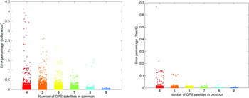
Figure 11. Positioning error distribution with difference (Left) and direct algorithms (Right).
Table 3. Comparison of the average error percentages.

3.4. Swap Day Results
On December 10, 2005, GRACE satellites switched positions: GRACE B took the leader position while GRACE A was repositioned as the “follower”. During the manoeuvre, the distance between the two satellites went down to an all-time low of about 400 m (see Figure 12). As the distance between GRACE A and GRACE B decreased, the number of GPS satellites that both of them had in view increased. As illustrated in Figure 13, 41·8% of the time, a minimum of eight common satellites were in sight (that proportion was as low as 12·7% for the three-day period previously considered).

Figure 12. Inter-satellite separation on swap day.

Figure 13. Distribution of the number of GPS satellites in common.
As the K-Band ranging system was deactivated on swap day, GNV data (ECEF positions of the GRACE satellites as provided by the Jet Propulsion Laboratory) were used as a ‘true’ reference. For the error calculations, the computed relative positioning data had to be sampled (1:6), since GNV data are given once every minute only. A cumulative distribution analysis (see Figure 14) confirmed the performance of the ‘direct’ algorithm. For example, 91·32% of the errors were smaller than a metre when using the ‘direct’ algorithm as opposed to 22·92% when using the ‘difference’ algorithm (see Table 4).

Figure 14. Cumulative error distributions.
Table 4. Cumulative errors comparison.

Figure 15 presents the error percentage on the relative distance between the GRACE satellites over time. The ‘direct’ algorithm allowed for the reduction of the average error percentage by two orders of magnitude: μdirect=1·53⋅10−2; μdifference=1·55.

Figure 15. Relative positioning error percentages with difference (Left) and direct (Right) algorithms.
4. CONCLUSION
An innovative method allowing for the calculation of the distance between two satellites was developed and validated. It is based on single-frequency pseudorange measurements only. Unlike other single-frequency algorithms, it does not feature differential operators and its foundation lies on pure vectorial geometry. The average relative positioning error could be reduced by up to two orders of magnitude. The concept of Relative Geometric Dilution of Precision (RGDOP), which takes into account the configuration of the GPS satellites in common, was introduced. The impact of the number of common satellites on the relative positioning errors and the RGDOP was also quantified. Although the accuracy level is not as good as that reached through carrier-phase methods, the technique exhibited in this article still provides a commendable precision and offers an ease of implementation and a substantial cost-reduction in relation to other methods.
ACKNOWLEDGEMENTS
The authors would like to thank Shan Mohiuddin (Cornell University), Gerard Kruizinga (NASA Jet Propulsion Laboratory) and Roni Waler (Asher Space Research Institute) for their unwavering help and express their gratitude to the Israeli Ministry of Scientific Integration and the European GNSS Supervisory Authority, without the funding of which this research would not have been made possible.
APPENDIX GPS Satellite Position Determination
The equations described in this section allow for the calculation of the GPS satellites' coordinates in the WGS-84 ECEF (Earth-Centred Earth-Fixed) reference frame. They do so without using any of the reciprocal trigonometric functions exhibited in Table 2.15 of Reference [6], which is a warranty for unambiguous computational results.
Let e denote the broadcast eccentricity, E k the calculated eccentric anomaly and νk the true anomaly. The true and eccentric anomalies are related as follows:
The argument of latitude Φk is defined as Φk=v k+ω, where ω represents the broadcast argument of perigee. The second harmonic perturbations (corrections to the argument of latitude, radius and inclination) can be written as linear functions of sin 2Φk and cos 2Φk:

where l s, l c, r s, r c, i s and i c respectively represent the broadcast latitude, radius and inclination correction coefficients.
νk and Φk do not need to be explicitly calculated to compute δl k, δr k and δi k. The terms sin 2Φk and cos 2Φk can be directly expressed as functions of sin νk and cos νk:
Similarly, the corrected argument of latitude l k=Φk+δl k does not have to be numerically computed. The terms cos l k and sin l k, needed to calculate the perifocal coordinates of each of the GPS satellites (i.e., the two-dimensional position in their respective orbital plane), can be expressed as:


