1. INTRODUCTION
Due to the special processing technology and design principles of a Micro-Electromechanical Systems (MEMS) gyroscope, the factors influencing the precision of its angular rate output are different from those of the traditional laser and fibre optic gyroscope (Lv et al., Reference Lv, Lai, Liu and Qin2014a). In the angular rate output of a MEMS gyroscope, there is a measurement error produced by the acceleration named g-sensitivity error (Weinberg, Reference Weinberg2011; Borenstein et al., Reference Borenstein, Ojeda and Kwanmuang2009). In applications for consumer and business use, the bias instability of a MEMS gyroscope is poor (Weinberg, Reference Weinberg2011; Borenstein et al., Reference Borenstein, Ojeda and Kwanmuang2009; El-Rabbany and El-Diasty, Reference El-Rabbany and El-Diasty2004), generally up to hundreds of degrees per hour, and the vast majority of applications are used in the low-dynamic environment with relatively small acceleration (less than 2 g), thus the gyroscope output error caused by the g-sensitivity error is smaller than other errors (such as the bias instability), so its influence on the navigation system is often overlooked. Therefore, there are few references about research on the calibration and compensation of g-sensitivity error in MEMS gyroscopes. In recent years, with the continuous improvement of the performance of MEMS gyroscopes, the bias instability of MEMS gyroscope output has been reduced (the bias instability of some products are a few degrees per hour, or even below one degree per hour), and these high-precision MEMS gyroscopes have reached the tactical standard (Perlmutter and Robin, Reference Perlmutter and Robin2012; Trusov, Reference Trusov2011; Xing et al., Reference Xing, Hang, Xiong, Liu and Wan2016). However, although the bias instability indices in some high-precision MEMS gyroscopes are very good, their g-sensitivity error coefficient indices differ by a factor of several tens (Wu et al., Reference Wu, Yao and Ma2013; Sensonor, 2015; MuRata, 2015). Therefore, past methods of evaluating the gyroscope performance with bias instability in laser and optical fibre gyroscopes are not accurate enough in the performance evaluation of MEMS gyroscopes (Lv et al., Reference Lv, Lai, Liu and Nie2014b; Peng et al., Reference Peng, Xiong, Wang, Liu and Zhang2014), especially in some high-dynamic application environments.
Due to the existence of g-sensitivity error in MEMS gyroscopes, this index and the vehicle acceleration will directly affect the actual performance of a high-precision MEMS gyroscope. Therefore, the g-sensitivity error coefficient of a MEMS gyroscope is also one of the important indicators affecting its actual performance. The angular rate output error in these high-precision MEMS gyroscopes caused by g-sensitivity error cannot be easily ignored, and needs calibration and compensation. In a previous study on MEMS gyroscope performance enhancement techniques, Park et al. (Reference Park, Han and Lee2015) studied the mechanism of production of g-sensitivity error, and improved the structure design of a MEMS gyroscope, so as to obtain a smaller g-sensitivity error coefficient, thus reducing the g-sensitivity error, but their method is not suitable for reducing the g-sensitivity error in a mature MEMS gyroscope or MEMS Inertial Measurement Unit (IMU).
Research on reducing the g-sensitivity error in existing MEMS gyroscopes includes building the g-sensitivity error model in the IMU (Yang et al., Reference Yang, El-Sheimy, Goodall and Niu2007). Based on the g-sensitivity error model the g-sensitivity error coefficients are expanded to the integrated filtering state and a high-dimension Kalman filter is built. Then the g-sensitivity error in the MEMS gyroscope is stimulated through a special movement mode, to realise the online estimation of g-sensitivity error coefficients and compensation of g-sensitivity error (Bancroft and Lachapelle, Reference Bancroft and Lachapelle2012; Fan et al., Reference Fan, Hu, He, Luo and Tang2013; Reference Fan, Hu, He, Tang and Luo2014). It has been verified in the literature that such an online calibration method for finding g-sensitivity error coefficients can improve the dynamic performance of a MEMS gyroscope, thus increasing the precision of integrated navigation. When estimating such a small g-sensitivity error coefficient in a high-dimension filter, the system complexity will be increased as the system needs to add another three or nine dimensions. On the other hand, a specific movement incentive needs to be designed to effectively stimulate the error; however it is difficult to guarantee that g-sensitivity error coefficients can be accurately estimated each time. In addition to the research on online calibration methods of g-sensitivity error coefficients, there is also some documented research on online calibration methods, there is also some research on a turntable experiment for high-precision MEMS gyroscopes, which realises the offline calibration of g-sensitivity error coefficients, so as to improve the MEMS gyroscope's measurement accuracy of rotational angular velocity of the Earth through the compensation of g-sensitivity error (Iozan et al., Reference Iozan, Collin, Pekkalin, Hautamäki, Takala and Rusu2010). Although the turntable calibration scheme of g-sensitivity error coefficients is given in Iozan et al. (Reference Iozan, Collin, Pekkalin, Hautamäki, Takala and Rusu2010), the specific calibration process and results are not discussed and validated in detail.
The MEMS gyroscope is a mechanical gyroscope, and the traditional calibration experiments of g-sensitivity error in mechanical gyroscopes are generally carried out on a high-precision centrifuge (Wang, Reference Wang2014). The calibration process is complex and the calibration conditions are harsh.
Therefore, there are three difficulties in the offline calibration of g-sensitivity error of a MEMS gyroscope. Firstly, the traditional calibration method of g-sensitivity error needs high-cost and high-precision calibration equipment. Thus, in the relatively low cost MEMS gyroscope application, the testing cost is relatively high and the calibration process is relatively complicated. Secondly, triaxial Earth rotation rate components measured by the MEMS gyroscope are difficult to obtain accurately, so they are difficult to separate from the g-sensitivity error, thus affecting the calibration of g-sensitivity error coefficients. Finally, the larger random noise and bias existing in MEMS gyroscopes (Cao et al., Reference Cao, Li and Kou2016), will also affect the calibration of g-sensitivity error coefficients. Considering the three aspects of the problem of the g-sensitivity error calibration in MEMS gyroscopes, we need to use low-cost calibration equipment and simple calibration processes as far as possible. Also, we need to investigate how to compensate the bias and random noise of the MEMS gyroscope, and how to eliminate the influence of the Earth rotation rate components, to accurately calibrate g-sensitivity error coefficients and improve the output precision of the MEMS gyroscope.
Based on the above analysis, this paper proposes a new and fast offline calibration method of g-sensitivity error coefficients for the existing high-precision MEMS gyroscope, to improve the precision and actual performance of high-performance MEMS gyroscopes. Through the analysis of a MEMS gyroscope output model containing the g-sensitivity error, we build a calibration model of g-sensitivity error coefficients, which effectively eliminates the influence of the Earth rotation rate components, and designs a special calibration experiment scheme at (8 + N) positions. By smoothing the MEMS IMU data collected at each position, the influence of random noise is eliminated. At the first eight symmetrical positions, the gyroscope bias is calibrated and thus can be compensated in the MEMS gyroscope output. On the basis of the calibration model and processed MEMS IMU data, the Newton iteration and least squares methods are adopted to fit g-sensitivity error coefficients. Finally, this work also designs many groups of calibration experiments for g-sensitivity error coefficients on the high-precision MEMS IMU system STIM300, to verify the effectiveness of the proposed calibration method of g-sensitivity error coefficients, and the stability and repeatability of the g-sensitivity error coefficients thus calibrated.
2. CALIBRATION METHODOLOGY
This section analyses the mechanism of g-sensitivity error in MEMS gyroscopes and derives the calibration models of g-sensitivity error coefficients based on the static error model of a MEMS gyroscope. Next, an (8 + N)-position calibration experiment scheme is designed, to counteract the influence of MEMS gyroscope bias and random noise on g-sensitivity error coefficients calibration. With respect to the non-linear characteristics of calibration model equations and the multi-parameter calibration requirement, the Newton iteration method is used for linearizing non-linear equations of calibration models, and then the least squares method is used for fitting g-sensitivity error coefficients.
2.1. Mechanism of g-sensitivity error and MEMS gyroscope error model analysis
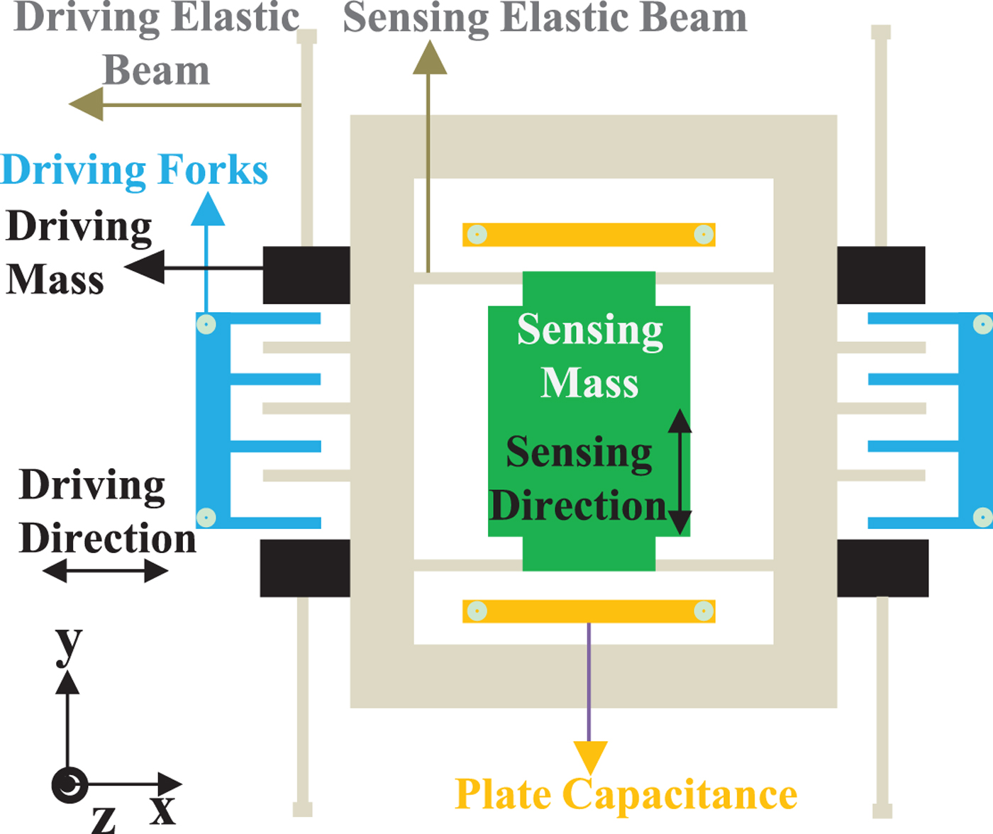
The working principles of MEMS gyroscopes are varied, but are mainly based on the physical principle of the vibration object sensing the angular velocity, namely using the vibration-induced mass blocks in MEMS gyroscopes to detect the Coriolis force and then converting the force to an angular rate output via the corresponding sensing signal processing unit. Silicon MEMS gyroscopes are the most common MEMS gyroscope products, and a simplified internal structure is shown in Figure 1. Its kinetic model can be equivalently simplified as an elastic damping system that drives mass blocks. Sensing mass blocks are suspended on the base of an elastic structure as shown in Figure 2.

Figure 1. Silicon MEMS gyroscope internal simple structure.
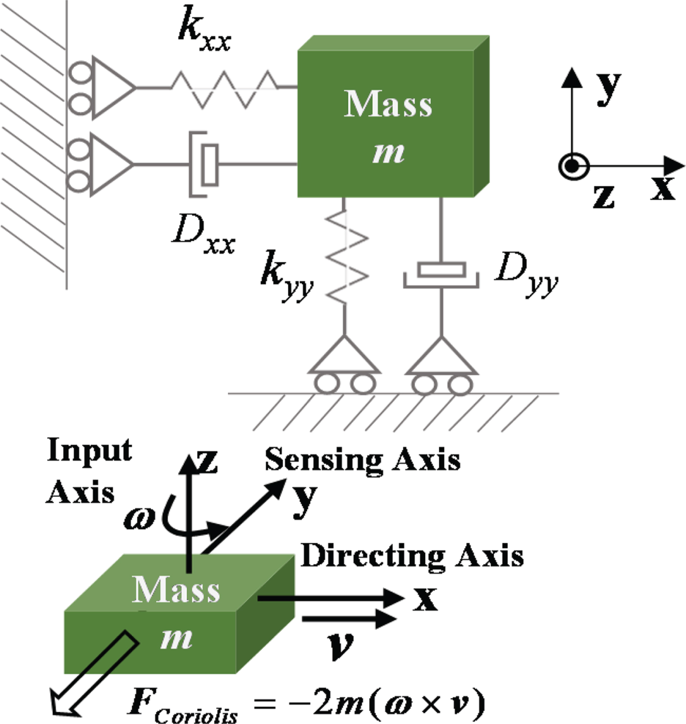
Figure 2. Silicon MEMS gyroscope equivalently simplified kinetic model
Assuming that the x-axis has a vibration velocity v and that the z-axis has an input angular rate ω , a Coriolis acceleration is generated on the y-axis and then a Coriolis F Coriolis force is generated on the mass. The Coriolis force expression is given in Equation (1).
 $${\bi F}_{Coriolis} = -2m \lpar {\bf \omega} \times {\bi v}\rpar $$
Seen from Equation (1), the core working principle of a MEMS gyroscope is that orthogonal vibration and rotation produce the Coriolis force, which is converted to corresponding capacitance or voltage changes, and then these corresponding capacitance or voltage changes are converted to the desired angular rate information by means of a control and rebalancing circuit to realise the measurement of the input angular rate. However, if the additional inertial force acted on mass blocks, the original Coriolis force
F
Coriolis
would be changed, which would cause an additional increase in the angular rate output and thus produce the MEMS gyroscope measurement error. The acceleration which produces the inertial external force is the ideal measurement output
f
b
of the accelerometer (Groves, Reference Groves2013) and thus the MEMS gyroscope measurement error is called g-sensitivity error due to
f
b
= −
g
b
under static conditions. The g-sensitivity error of the MEMS gyroscope output is given in Equation (2), where
 ${\bf G} = \left[\matrix{G_{xx} & G_{xy} & G_{xz} & G_{yx} & G_{yy} & G_{yz} & G_{zx} & G_{zy} & G_{zz}} \right]$
are the g-sensitivity error coefficients.
${\bf G} = \left[\matrix{G_{xx} & G_{xy} & G_{xz} & G_{yx} & G_{yy} & G_{yz} & G_{zx} & G_{zy} & G_{zz}} \right]$
are the g-sensitivity error coefficients.
 $${\bi G}_{\omega}^b = \left[\matrix{G_{xx} & G_{xy} & G_{xz} \cr G_{yx} & G_{yy} & G_{yz} \cr G_{zx} & G_{zy} & G_{zz}}\right]$$
According to the influence of different error sources on the MEMS gyroscope, its angular rate output error mainly includes bias ε b , g-sensitivity error G ω b , scale factor error, installation error A b and random noise η b (Liu., Reference Liu2004). The MEMS gyro error model Δ ω b containing these errors is shown in Equation (3).
 $$\Delta {\bf \omega}^b = {\bf \varepsilon}^b + {\bi G}_{\omega}^b + {\bi A}^b + {\bf \eta}^b $$
From Equation (3), to improve the output accuracy of a MEMS gyroscope, not only ε b and A b (Aggarwal et al., Reference Aggarwal, Syed, Niu and El-Sheimy2008) should be calibrated, but also the g-sensitivity error G ω b should be calibrated, especially for a few high-precision MEMS gyroscope products. This is due to improvements of high-precision MEMS gyroscope design and manufacturing technology. Bias stability has gradually been improved and thus the proportion of g-sensitivity error is more and more obvious in the angular rate measurement error.
2.2. Calibration models of g-sensitivity error coefficients
It can be seen from Equation (3) that these errors are mutually coupled and scale factor error and installation error
A
b
can be almost negligible under the static condition. Equation (4) shows a MEMS gyroscope triaxial output model including g-sensitivity error under the static condition. Since the research object is the high-precision MEMS gyroscope, its bias instability is a few degrees or even below one degree per hour, thus its measurement output can obviously reflect rotational angular velocity of the Earth under the static condition, compared with the low-precision MEMS gyroscope. As a result, Equation (4) contains the triaxial component of rotational angular velocity of the Earth on the sensor coordinate b expressed as ω
iex
b
, ω
iey
b
and ω
iez
b
, g-sensitivity error
G
ω
b
, gyroscope bias
 ${\bf \varepsilon}^{b} = \left[\matrix{\varepsilon_{x}^{b} & \varepsilon_{y}^{b} & \varepsilon_{z}^{b}}\right]$
and random noise
${\bf \varepsilon}^{b} = \left[\matrix{\varepsilon_{x}^{b} & \varepsilon_{y}^{b} & \varepsilon_{z}^{b}}\right]$
and random noise
 ${\bf \eta}^{b} = \left[\matrix{\eta_{x}^{b} & \eta_{y}^{b} & \eta_{z}^{b}}\right]$
. In Equation (4),
${\bf \eta}^{b} = \left[\matrix{\eta_{x}^{b} & \eta_{y}^{b} & \eta_{z}^{b}}\right]$
. In Equation (4),
 ${\bf f}^{b} = \left[\matrix{f_{x}^{b} &f_{y}^{b} &f_{z}^{b}} \right]$
is the MEMS acceleration output and
${\bf f}^{b} = \left[\matrix{f_{x}^{b} &f_{y}^{b} &f_{z}^{b}} \right]$
is the MEMS acceleration output and
 ${\bf \omega}^{b} = \left[\matrix{ \omega_{x}^{b} & \omega_{y}^{b} & \omega_{z}^{b}}\right]$
is the MEMS gyroscope output.
${\bf \omega}^{b} = \left[\matrix{ \omega_{x}^{b} & \omega_{y}^{b} & \omega_{z}^{b}}\right]$
is the MEMS gyroscope output.
 $$\left\{\matrix{\omega_x^b = \omega_{iex}^b + G_{xx} f_x^b + G_{xy} f_y^b + G_{xz} f_z^b + \varepsilon_x^b + \eta_x^b \cr \omega_y^b = \omega_{iey}^b + G_{yx} f_x^b + G_{yy} f_y^b + G_{yz} f_z^b + \varepsilon_y^b + \eta_y^b \cr \omega_z^b = \omega_{iez}^b + G_{zx} f_x^b + G_{zy} f_y^b + G_{zz} f_z^b + \varepsilon_z^b + \eta_z^b \cr}\right. $$
By transforming Equation (4) and marking
 $G_{xx} f_{x}^{b} + G_{xy} f_{y}^{b} + G_{xz} f_{z}^{b}$
,
$G_{xx} f_{x}^{b} + G_{xy} f_{y}^{b} + G_{xz} f_{z}^{b}$
,
 $G_{yx} f_{x}^{b} + G_{yy} f_{y}^{b} + G_{yz} f_{z}^{b}$
and
$G_{yx} f_{x}^{b} + G_{yy} f_{y}^{b} + G_{yz} f_{z}^{b}$
and
 $G_{zx} f_{x}^{b} + G_{zy} f_{y}^{b} + G_{zz} f_{z}^{b}$
simply as C
1, C
2 and C
3, Equation (5) is derived as:
$G_{zx} f_{x}^{b} + G_{zy} f_{y}^{b} + G_{zz} f_{z}^{b}$
simply as C
1, C
2 and C
3, Equation (5) is derived as:
 $$\left\{\matrix{\omega_{iex}^b = \omega_x^b - C_{1} - \varepsilon_x^b - \eta_x^b \cr \omega_{iey}^b = \omega_y^b - C_{2} - \varepsilon_y^b - \eta_y^b \cr \omega_{iez}^b = \omega_z^b - C_{3} - \varepsilon_z^b - \eta_z^b }\right. $$
When both sides of the three equations are squared and then summed, the left of the equation derived is
 $\lpar \omega_{iex}^{b}\rpar ^{2} + \lpar \omega_{iey}^{b}\rpar ^{2} + \lpar \omega_{iez}^{b}\rpar ^{2}$
and then the square root of the equation derived is calculated. Thus, the left of the latest equation derived is
$\lpar \omega_{iex}^{b}\rpar ^{2} + \lpar \omega_{iey}^{b}\rpar ^{2} + \lpar \omega_{iez}^{b}\rpar ^{2}$
and then the square root of the equation derived is calculated. Thus, the left of the latest equation derived is
 $\sqrt{\lpar \omega_{iex}^{b}\rpar ^{2} + \lpar \omega_{iey}^{b}\rpar ^{2} + \lpar \omega_{iez}^{b}\rpar ^{2}}$
, equalling the modular value of rotational angular velocity of the Earth ω
ie
. The latest equation derived is shown as Equation (6), where C
1, C
2, C
3 contain nine g-sensitivity error coefficients.
$\sqrt{\lpar \omega_{iex}^{b}\rpar ^{2} + \lpar \omega_{iey}^{b}\rpar ^{2} + \lpar \omega_{iez}^{b}\rpar ^{2}}$
, equalling the modular value of rotational angular velocity of the Earth ω
ie
. The latest equation derived is shown as Equation (6), where C
1, C
2, C
3 contain nine g-sensitivity error coefficients.
 $$\omega_{ie} = \sqrt{\lpar \omega_x^b - C_{1} - \varepsilon_x^b - \eta_x^b \rpar ^2 + \lpar \omega_y^b - C_{2} - \varepsilon_y^b - \eta_y^b \rpar ^2 + \lpar \omega_z^b - C_{3} - \varepsilon_z^b - \eta_z^b \rpar ^2} $$
If the MEMS gyroscope was started, more than nine output groups would be acquired, which would and then constitute a set of nonlinear equations composed of more than nine equations in the form of Equation (6). By solving the nonlinear equations, the nine coefficients can be calculated. Meanwhile, the least squares method is used to solve the nine coefficients from the overdetermined and linearized equations, the number of which is equal to or greater than nine. Therefore, in Section 2.4, the theoretical derivation for fitting the nine g-sensitivity error coefficients is given with the application of the Newton iteration and least squares methods.
In Equation (6), the triaxial bias of a MEMS gyroscope
 ${\bf \varepsilon}^{b} = \left[\matrix{\varepsilon_{x}^{b} & \varepsilon_{y}^{b} & \varepsilon_{z}^{b}}\right]$
and random noise
${\bf \varepsilon}^{b} = \left[\matrix{\varepsilon_{x}^{b} & \varepsilon_{y}^{b} & \varepsilon_{z}^{b}}\right]$
and random noise
 ${\bf \eta}^{b} = \left[\matrix{ \eta_{x}^{b} & \eta_{y}^{b} & \eta_{z}^{b}}\right]$
is unknown, so the bias and random noise should be compensated from the output of the MEMS gyroscope, to offset their effects on calibrating g-sensitivity error coefficients. Moreover, as seen from Equation (4), g-sensitivity error is related to MEMS accelerometer output, thus if the raw output of the MEMS accelerometer is directly used in the g-sensitivity error coefficients calibration process, its random noise would also affect the calibrated values. Accordingly, MEMS accelerometer random noise should also be compensated. Based on the above analysis, a multi-position calibration experiment scheme should be designed, and then the output data of a MEMS IMU should be collected and processed in the calibration experiment. The purpose of such a scheme design is to calibrate the nine g-sensitivity error coefficients from more than nine calibration equations, offsetting random noise of the MEMS gyroscope and accelerometer and compensating gyroscope bias error. Thus, Section 2.3 designs a special (8 + N)-position calibration experiment scheme.
${\bf \eta}^{b} = \left[\matrix{ \eta_{x}^{b} & \eta_{y}^{b} & \eta_{z}^{b}}\right]$
is unknown, so the bias and random noise should be compensated from the output of the MEMS gyroscope, to offset their effects on calibrating g-sensitivity error coefficients. Moreover, as seen from Equation (4), g-sensitivity error is related to MEMS accelerometer output, thus if the raw output of the MEMS accelerometer is directly used in the g-sensitivity error coefficients calibration process, its random noise would also affect the calibrated values. Accordingly, MEMS accelerometer random noise should also be compensated. Based on the above analysis, a multi-position calibration experiment scheme should be designed, and then the output data of a MEMS IMU should be collected and processed in the calibration experiment. The purpose of such a scheme design is to calibrate the nine g-sensitivity error coefficients from more than nine calibration equations, offsetting random noise of the MEMS gyroscope and accelerometer and compensating gyroscope bias error. Thus, Section 2.3 designs a special (8 + N)-position calibration experiment scheme.
2.3. (8 + N)-position calibration experiment scheme
Based on the detailed calibration model analysis of g-sensitivity error coefficients in Section 2.2, it can be concluded that, before calibrating the nine g-sensitivity error coefficients, multi-position experiments need to be designed to compensate the bias ε b and random noise of the gyroscope and accelerometer. η b and random noise of the MEMS accelerometer in Equations (4)–(6) mainly contain quantisation noise and white noise, which can be counteracted by smoothing the static MEMS IMU output collected for a period at each position. As for calibrating the gyroscope bias ε b , we usually rotate the three axes of the gyroscope to a plurality of symmetrical positions using a 180° rotation, to offset the impact of rotational angular velocity of the Earth; thus the bias is calibrated. In the process of calibration of the gyroscope bias shown in Equation (4), not only the impact of rotational angular velocity of the Earth but also the influence of g-sensitivity error should be considered. Hence, traditional multi-position calibration experiments should be improved and optimised, to simultaneously offset the impact of rotational angular velocity of the Earth and g-sensitivity error. Thus, the (8 + N(N ≥ 1))-position calibration experiment scheme is designed as shown in Figure 3.

Figure 3. (8 + N(N ≥ 1))-position calibration experiment scheme.
Among the (8 + N(N ≥ 1)) positions designed in Figure 4, the first eight positions designed are mainly used for calibrating the gyroscope bias. At each position, the static output data of the MEMS IMU are collected for a period and then smoothed to reduce the influence of random noise on the calibration results.

Figure 4. (8 + N(N ≥ 1)) calibration positions diagram.
The reason for designing the eight calibration positions can be explained by the x-axis gyroscope bias calibration process. Equation (7) gives the relationship of the rotational angular velocity component of the Earth at each position and Equation (8) shows the relationship of the three-axis output of the MEMS accelerometer at each position.
 $$\eqalign{\omega_{iex}^{b\lpar 1\rpar } & = -\omega_{iex}^{b\lpar 3\rpar } = -\omega_{iex}^{b\lpar 5\rpar } = \omega_{iex}^{b\lpar 7\rpar } \cr \omega_{iey}^{b\lpar 1\rpar } &= -\omega_{iex}^{b\lpar 2\rpar } = \omega_{iex}^{b\lpar 4\rpar } = -\omega_{iex}^{b\lpar 6\rpar } = \omega_{iex}^{b\lpar 8\rpar } \cr f_x^{b\lpar 1\rpar } & = f_y^{b\lpar 2\rpar } = - f_x^{b\lpar 3\rpar } = -f_y^{b\lpar 4\rpar } = -f_x^{b\lpar 5\rpar } \cr & = -f_y^{b\lpar 6\rpar } = f_x^{b\lpar 7\rpar } = f_y^{b\lpar 8\rpar }} $$
 $$\eqalign{f_y^{b\lpar 1\rpar } &= -f_x^{b\lpar 2\rpar } = -f_y^{b\lpar 3\rpar } = f_x^{b\lpar 4\rpar } = f_y^{b\lpar 5\rpar } \cr & = -f_x^{b\lpar 6\rpar } = -f_y^{b\lpar 7\rpar } = f_x^{b\lpar 8\rpar } \cr f_z^{b\lpar 1\rpar } & = f_z^{b\lpar i\rpar }\comma \; \lpar i = 2\comma \; 3\comma \; 4\rpar \cr &= -f_z^{b\lpar j\rpar } \lpar j = 5\comma \; 6\comma \; 7\comma \; 8\rpar }$$
We plug Equation (7) and Equation (8) into Equation (4) respectively and re-express the x-axis gyroscope output as
 $\tilde{\omega}_{x}^{b}$
, which is without random noise.
$\tilde{\omega}_{x}^{b}$
, which is without random noise.
 $\tilde{\omega}_{x}^{b}$
of the eight positions can be expressed as Equation (9) and Equation (10):
$\tilde{\omega}_{x}^{b}$
of the eight positions can be expressed as Equation (9) and Equation (10):
 $$\eqalign{\tilde{\omega}_x^{b\lpar 1\rpar } &= {\omega}_{iex}^{b\lpar 1\rpar } + G_{xx} f_x^{b\lpar 1\rpar } + G_{xy} f_y^{b\lpar 1\rpar } + G_{xz} f_z^{b\lpar 1\rpar } + \varepsilon_x^b \cr \tilde{\omega}_x^{b\lpar 2\rpar } &= -{\omega}_{iey}^{b\lpar 1\rpar } + G_{xx} \lpar -f_y^{b\lpar 1\rpar } \rpar + G_{xy} f_y^{b\lpar 1\rpar } + G_{xz} f_z^{b\lpar 1\rpar } + \varepsilon_x^b \cr \tilde{\omega}_x^{b\lpar 3\rpar } & = -{\omega}_{iex}^{b\lpar 1\rpar } + G_{xx} \lpar -f_x^{b\lpar 1\rpar } \rpar + G_{xy} \lpar -f_y^{b\lpar 1\rpar } \rpar + G_{xz} f_z^{b\lpar 1\rpar } + \varepsilon_x^b \cr \tilde{\omega}_x^{b\lpar 4\rpar } & = {\omega}_{iey}^{b\lpar 1\rpar } + G_{xx} f_y^{b\lpar 1\rpar } + G_{xy} \lpar -f_x^{b\lpar 1\rpar } \rpar + G_{xz} f_z^{b\lpar 1\rpar } + \varepsilon_x^b} $$
 $$\eqalign{\tilde{\omega}_x^{b\lpar 5\rpar } &= -{\omega}_{iex}^{b\lpar 1\rpar } + G_{xx} \lpar -f_x^{b\lpar 1\rpar } \rpar + G_{xy} f_y^{b\lpar 1\rpar } + G_{xz} \lpar -f_z^{b\lpar 1\rpar } \rpar + \varepsilon_x^b \cr \tilde{\omega}_x^{b\lpar 6\rpar } &= -{\omega}_{iey}^{b\lpar 1\rpar } + G_{xx} \lpar -f_y^{b\lpar 1\rpar } \rpar + G_{xy} \lpar -f_x^{b\lpar 1\rpar } \rpar + G_{xz} \lpar -f_z^{b\lpar 1\rpar } \rpar + \varepsilon_x^b \cr \tilde{\omega}_x^{b\lpar 7\rpar } & = {\omega}_{iex}^{b\lpar 1\rpar } + G_{xx} f_x^{b\lpar 1\rpar } + G_{xy} \lpar -f_y^{b\lpar 1\rpar } \rpar + G_{xz} \lpar -f_z^{b\lpar 1\rpar } \rpar + \varepsilon_x^b \cr \tilde{\omega}_x^{b\lpar 8\rpar } & = {\omega}_{iey}^{b\lpar 1\rpar } + G_{xx} f_y^{b\lpar 1\rpar } + G_{xy} f_x^{b\lpar 1\rpar } + G_{xz} \lpar -f_z^{b\lpar 1\rpar } \rpar + \varepsilon_x^b} $$
Equations (11) and (12) are derived by summing each equation in Equations (9) and (10) respectively, and then both sides of Equations (11) and (12) are summed. Thus, the gyroscope x-axis bias is calculated as shown in Equation (13). Similarly, the y-axis and z-axis gyroscope bias can be also calibrated. From the process of calibration and calibration value of ε x b , it can be seen that designing the first eight symmetrical positions can effectively offset the influence of the angular velocity of the Earth and g-sensitivity error in calibrating the gyro bias error. Thus, the gyro bias error can be calibrated and compensated accurately. Although the eight-position design is not unique, with such a design, the impact of the rotational angular velocity of the Earth and g-sensitivity error in calibrating the bias can be simply and intuitively derived and offset.
 $$\tilde{\omega}_x^{b\lpar 1\rpar } + \tilde{\omega}_x^{b\lpar 2\rpar } + \tilde{\omega}_x^{b\lpar 3\rpar } + \tilde{\omega}_x^{b\lpar 4\rpar } = 4G_{xz} f_z^{b\lpar 1\rpar } + 4\varepsilon_x^b $$
 $$\tilde{\omega}_x^{b\lpar 5\rpar } + \tilde{\omega}_x^{b\lpar 6\rpar } + \tilde{\omega}_x^{b\lpar 7\rpar } + \tilde{\omega}_x^{b\lpar 8\rpar } = 4G_{xz} \lpar -f_z^{b\lpar 1\rpar } \rpar + 4\varepsilon_x^b $$
 $$\varepsilon_x^b = \left(\sum_{i=1}^{8} \tilde{\omega}_x^{b\lpar i\rpar } \right)\bigg{/}8 $$
From Equation (4), it can be seen that the number of g-sensitivity error coefficients is nine. As a result, in addition to designing the first eight positions, it is necessary to design at least one additional position to calibrate the nine parameters, and the other positions should not be coincident with the first eight positions. Figure 2 shows the ninth position design when N = 1. The MEMS gyroscope output of the i − th (i = 1,2…(8 + N)) position is re-expressed as
 ${\mathop{\omega}\limits^{\frown}}^{b\lpar i\rpar }$
after compensating random noise and the bias, and substituted into Equation (6). Thus, we obtain Equation (14) with (8 + N) equations in the form of Equation (6).
${\mathop{\omega}\limits^{\frown}}^{b\lpar i\rpar }$
after compensating random noise and the bias, and substituted into Equation (6). Thus, we obtain Equation (14) with (8 + N) equations in the form of Equation (6).
 $$\left\{\matrix{\omega_{ie} = \sqrt{\lpar {\mathop{\omega}\limits^{\frown}}_x^{b\lpar 1\rpar } - C_1 \rpar^2 + \lpar {\mathop{\omega}\limits^{\frown}}_y^{b\lpar 1\rpar } - C_2 \rpar^2 + \lpar {\mathop{\omega}\limits^{\frown}}_z^{b\lpar 1\rpar } - C_3 \rpar^2} \cr \qquad \qquad \qquad \qquad \qquad \qquad \vdots \cr \omega_{ie} = \sqrt{\lpar {\mathop{\omega}\limits^{\frown}}_x^{b\lpar i\rpar } - C_1 \rpar^2 + \lpar {\mathop{\omega}\limits^{\frown}}_y^{b\lpar i\rpar } - C_2 \rpar^2 + \lpar {\mathop{\omega}\limits^{\frown}}_z^{b\lpar i\rpar } - C_3 \rpar^2} \cr \qquad \qquad \qquad \qquad \qquad \qquad \vdots \cr \omega_{ie} = \sqrt{\lpar {\mathop{\omega}\limits^{\frown}}_x^{b\lpar 8 + N\rpar } - C_1 \rpar^2 + \lpar {\mathop{\omega}\limits^{\frown}}_y^{b\lpar 8 + N\rpar } - C_2 \rpar^2 + \lpar {\mathop{\omega}\limits^{\frown}}_z^{b\lpar 8 + N\rpar } - C_3 \rpar^2}}\right. $$
To calculate the nine g-sensitivity error coefficients from the nonlinear equations of Equation (14), we adopt the Newton iteration and least squares methods.
2.4. Fitting process of g-sensitivity error coefficients
Firstly, we use the Newton iteration method to convert Equation (14) into linear equations to calculate the coefficients. In the k-th Newton iteration of the data collected at the i-th position, the first order Taylor expansion of the i-th equation in Equation (14) is shown as Equation (15), where
 $f_{k}^{\lpar i\rpar } = \sqrt{\lpar {\mathop{\omega}\limits^{\frown}}_{x}^{b\lpar i\rpar } - C_{1\comma k}^{\lpar i\rpar } \rpar ^{2} + \lpar {\mathop{\omega}\limits^{\frown}}_{y}^{b\lpar i\rpar } - C_{2\comma k}^{\lpar i\rpar } \rpar ^{2} + \lpar {\mathop{\omega}\limits^{\frown}}_{z}^{b\lpar i\rpar } - C_{3\comma k}^{\lpar i\rpar } \rpar ^{2}}$
and
$f_{k}^{\lpar i\rpar } = \sqrt{\lpar {\mathop{\omega}\limits^{\frown}}_{x}^{b\lpar i\rpar } - C_{1\comma k}^{\lpar i\rpar } \rpar ^{2} + \lpar {\mathop{\omega}\limits^{\frown}}_{y}^{b\lpar i\rpar } - C_{2\comma k}^{\lpar i\rpar } \rpar ^{2} + \lpar {\mathop{\omega}\limits^{\frown}}_{z}^{b\lpar i\rpar } - C_{3\comma k}^{\lpar i\rpar } \rpar ^{2}}$
and
 $G_{j\comma k}^{\lpar i\rpar }\ \lpar j = 1\comma \; 2 \ldots 9\rpar $
is given in Equation (16) respectively.
$G_{j\comma k}^{\lpar i\rpar }\ \lpar j = 1\comma \; 2 \ldots 9\rpar $
is given in Equation (16) respectively.
 $$\eqalign{\omega_{ie} & = f_k^{\lpar i\rpar } + G_{1\comma k}^{\lpar i\rpar } \lpar G_{xx} - G_{xx\comma k} \rpar + G_{2\comma k}^{\lpar i\rpar } \lpar G_{xy} - G_{xy\comma k} \rpar + G_{3\comma k}^{\lpar i\rpar } \lpar G_{xz} - G_{xz\comma k} \rpar \cr & \quad + G_{4\comma k}^{\lpar i\rpar } \lpar G_{yx} - G_{yx\comma k} \rpar + G_{5\comma k}^{\lpar i\rpar } \lpar G_{yy} - G_{yy\comma k} \rpar + G_{6\comma k}^{\lpar i\rpar } \lpar G_{yz} - G_{yz\comma k} \rpar \cr & \quad + G_{7\comma k}^{\lpar i\rpar } \lpar G_{zx} - G_{zx\comma k} \rpar + G_{8\comma k}^{\lpar i\rpar } \lpar G_{zy} - G_{zy\comma k} \rpar + G_{9\comma k}^{\lpar i\rpar } \lpar G_{zz} - G_{zz\comma k} \rpar } $$
 $$\eqalign{G_{j\comma k}^{\lpar i\rpar } & = \displaystyle{{\partial f_k^{\lpar i\rpar }}\over{\partial G_{xm}}} = -\displaystyle{{f_m^{b\lpar i\rpar }\lpar {\mathop{\omega}\limits^{\frown}}_x^{b\lpar i\rpar } - C_{1\comma k}^{\lpar i\rpar } \rpar }\over{f_k^{\lpar i\rpar }}}\comma \; \lpar \lsqb j\comma \; m \rsqb = \lpar \lsqb 1\comma \; x \rsqb \comma \; \lsqb 2\comma \; y \rsqb \comma \; \lsqb 3\comma \; z \rsqb \rpar \rpar \cr G_{j\comma k}^{\lpar i\rpar } & = \displaystyle{{\partial f_k^{\lpar i\rpar }}\over{\partial G_{ym}}} = - \displaystyle{{f_m^{b\lpar i\rpar } \lpar {\mathop{\omega}\limits^{\frown}}_y^{b\lpar i\rpar } - C_{2\comma k}^{\lpar i\rpar } \rpar }\over{f_k^{\lpar i\rpar }}}\comma \; \lpar \lsqb j\comma \; m \rsqb = \lpar \lsqb 4\comma \; x \rsqb \comma \; \lsqb 5\comma \; y \rsqb \comma \; \lsqb 6\comma \; z \rsqb \rpar \rpar \cr G_{j\comma k}^{\lpar i\rpar } & = \displaystyle{{\partial f_k^{\lpar i\rpar }}\over{\partial G_{zm}}} = -\displaystyle{{f_m^{b\lpar i\rpar }\lpar {\mathop{\omega}\limits^{\frown}}_z^{b\lpar i\rpar } - C_{3\comma k}^{\lpar i\rpar } \rpar } \over{f_x^{\lpar i\rpar }}}\comma \; \lpar \lsqb j\comma \; m \rsqb = \lpar \lsqb 7\comma \; x \rsqb \comma \; \lsqb 8\comma \; y \rsqb \comma \; \lsqb 9\comma \; z \rsqb \rpar \rpar }$$
With the above conversion process, all the nonlinear equations in Equation (14) are converted into linear equations. The converted linear equations at the k-th Newton iteration are as shown in Equation (17), where the expression of G , Δ X and B are given in Equation (18), Equation (19) and Equation (20) respectively.
 $${\bi G} \Delta {\bi X} = {\bi B} $$
 $${\bi G} = \left[\matrix{ G_{1\comma k}^{\lpar 1\rpar } & G_{2\comma k}^{\lpar 1\rpar } &\ldots & G_{9\comma k}^{\lpar 1\rpar } \cr G_{1\comma k}^{\lpar 2\rpar } & G_{2\comma k}^{\lpar 2\rpar } &\ldots & G_{9\comma k}^{\lpar 2\rpar } \cr \ldots &\ldots &\ldots &\ldots \cr G_{1\comma k}^{\lpar 8 + N\rpar } & G_{2\comma k}^{\lpar 8 + N\rpar } &\ldots & G_{9\comma k}^{\lpar 8 + N\rpar }} \right]_{\lpar 8 + N\rpar \times 9} $$
 $$\eqalign{\Delta {\bi X} & = \lsqb G_{xx} - G_{xx\comma k}\comma \; G_{xy} - G_{xy\comma k}\comma \; G_{xz} - G_{xz\comma k}\comma \; \ldots \cr & \quad G_{yx} - G_{yx\comma k}\comma \; G_{yy} - G_{yy\comma k}\comma \; G_{yz} - G_{yz\comma k}\comma \; \ldots \cr & \quad G_{zx} - G_{zx\comma k}\comma \; G_{zy} - G_{zy\comma k}\comma \; G_{zz} - G_{zz\comma k} \rsqb _{1 \times 9}^{T}} $$
 $${\bi B} = \left[\matrix{\omega_{ie} - f_k^{\lpar 1\rpar } \cr \omega_{ie} - f_k^{\lpar 2\rpar } \cr \vdots \cr \omega_{ie} - f_k^{\lpar 8 + N\rpar }} \right]_{\lpar 8 + N\rpar \times 1} $$
In accordance with the least squares method solving rule, the solution of Equation (17) is expressed as Δ
X
= (
G
T
G
)
G
T
B
, by which Δ
X
can be solved in every iteration and then the module value ‖Δ
X
‖ can be solved. When ‖Δ
X
‖ satisfies the condition of ‖Δ
X
‖ ≤ ‖Δ
X
‖
threshold
in the n-th iteration, the iteration process is over. ‖Δ
X
‖
threshold
is the setting threshold value and now
 ${\bi G} = \left[\matrix{ G_{xx} &G_{xy} &G_{xz} &G_{yx} &G_{yy} &G_{yz} &G_{zx} &G_{zy} &G_{zz}}\right]$
in Δ
X
are the nine calibrated g-sensitivity error coefficients.
${\bi G} = \left[\matrix{ G_{xx} &G_{xy} &G_{xz} &G_{yx} &G_{yy} &G_{yz} &G_{zx} &G_{zy} &G_{zz}}\right]$
in Δ
X
are the nine calibrated g-sensitivity error coefficients.
2.5. Compensation of g-sensitivity error
With the fitting solutions
 ${\bi G} = \left[\matrix{ G_{xx} &G_{xy} G_{xz} &G_{yx} &G_{yy} &G_{yz} &G_{zx} &G_{zy} & G_{zz}}\right]$
of g-sensitivity error coefficients in Section 2.4, the g-sensitivity error of each axis of the MEMS gyroscope output collected at each position can be compensated by using Equation (21), where Δω
x
b
, Δω
y
b
and Δω
z
b
are the three-axis gyroscope remaining outputs after deducting the g-sensitivity error from
${\bi G} = \left[\matrix{ G_{xx} &G_{xy} G_{xz} &G_{yx} &G_{yy} &G_{yz} &G_{zx} &G_{zy} & G_{zz}}\right]$
of g-sensitivity error coefficients in Section 2.4, the g-sensitivity error of each axis of the MEMS gyroscope output collected at each position can be compensated by using Equation (21), where Δω
x
b
, Δω
y
b
and Δω
z
b
are the three-axis gyroscope remaining outputs after deducting the g-sensitivity error from
 ${\mathop{\bf \omega}\limits^{\frown}}^{b}$
.
${\mathop{\bf \omega}\limits^{\frown}}^{b}$
.
 $$\left\{\matrix{\Delta {\omega}_x^{b\lpar i\rpar } = {\mathop{\omega}\limits^{\frown}}_x^{b\lpar i\rpar } - G_{xx} f_x^{b\lpar 1\rpar } - G_{xy} f_y^{b\lpar i\rpar } - G_{xz} f_z^{b\lpar i\rpar } \cr \Delta {\omega}_y^{b\lpar i\rpar } = {\mathop{\omega}\limits^{\frown}}_y^{b\lpar i\rpar } - G_{yx} f_x^{b\lpar 1\rpar } - G_{yy} f_y^{b\lpar i\rpar } - G_{yz} f_z^{b\lpar i\rpar } \cr \Delta {\omega}_z^{b\lpar i\rpar } = {\mathop{\omega}\limits^{\frown}}_z^{b\lpar i\rpar } - G_{zx} f_x^{b\lpar 1\rpar } - G_{zy} f_y^{b\lpar i\rpar } - G_{zz} f_z^{b\lpar i\rpar }}\right. $$
If the g-sensitivity error was compensated accurately, the three-axis gyroscope remaining outputs Δω x b , Δω y b and Δω z b would be equal to the rotational angular velocity component of the Earth respectively, namely, the modular value of the three-axis gyroscope remaining output at each position would be equal to ω ie , which is the modular value of the rotational angular velocity of the Earth. The calculation of ‖Δ ω b(i)‖ is as shown in Equation (22).
 $$\Vert \Delta {{\bf \omega}}^{b\lpar i\rpar } \Vert = \sqrt{\lpar \Delta {\omega}_x^{b\lpar i\rpar } \rpar ^2 + \lpar \Delta {\omega}_y^{b\lpar i\rpar } \rpar ^2 \lpar \Delta {\omega}_z^{b\lpar i\rpar } \rpar ^2}\comma \; i = 1\comma \; 2 \ldots \lpar 8 + N\rpar $$
The error between ‖Δ ω b(i)‖ and ω ie is recorded as Δω ie_after (i), and compared with the error before the g-sensitivity error compensation, to verify and evaluate the g-sensitivity error compensation effect. The calculation of Δω ie_after (i) and Δω ie_before (i) is given in Equations (23) and (24), respectively. If Δω ie_after (i) < Δω ie_before (i), this would verify that the compensation of the g-sensitivity error is effective. Moreover, the smaller Δω ie_after (i) was compared with Δω ie_before (i), the better the compensation effect would be.
 $$\Delta {\omega}_{ie\_after}^{\lpar i\rpar } = \vert \Vert \Delta {{\bf \omega}}^{b\lpar i\rpar } \Vert - \omega_{ie} \vert \comma \; i = 1 \cdots \lpar 8 + N\rpar $$
 $$\Delta {\omega}_{ie\_before}^{\lpar i\rpar } = \left\vert \sqrt{\lpar {\mathop{\omega}\limits^{\frown}}_x^{b\lpar i\rpar } \rpar^2 + \lpar {\mathop{\omega}\limits^{\frown}}_y^{b\lpar i\rpar } \rpar^2 + \lpar {\mathop{\omega}\limits^{\frown}}_z^{b\lpar i\rpar } \rpar^2} -\omega_{ie}\right\vert $$
3. EXPERIMENT DESIGN AND RESULTS
To verify the g-sensitivity error calibration method proposed, the high-precision MEMS IMU system STIM300 is adopted to conduct the (8 + N) position calibration experiment. In STIM300, the bias instability of MEMS gyroscope is about 1°/h. When the gyroscope bias in STIM300 is calibrated and compensated under the static condition, the g-sensitivity error would still cause a fixed deviation of the gyroscope output. Thus, it is necessary to calibrate the g-sensitivity error coefficients of the gyroscope in STIM300, and compensate for the gyroscope output error caused by it, to improve the output accuracy of the MEMS gyroscope in STIM300, thus validating the effectiveness of the calibration method proposed.
The designed (8 + N)-position turntable experiment can verify not only the effectiveness of the proposed method but also the stability of the g-sensitivity error coefficients calibrated. Moreover, to analyse the effectiveness of this g-sensitivity error coefficients calibration method under arbitrary MEMS IMU attitudes, we designed multi-group contrast verification experiments of this g-sensitivity error compensation at arbitrary positions. Repeatability verification experiments of g-sensitivity coefficients were also designed.
3.1. STIM300 Data acquisition and processing of 16-position turntable experiment
In the stability verification experiments for calibrations of g-sensitivity coefficients, N = 8 in (8 + N) turntable positions; in other words, 16 positions are designed to calibrate the g-sensitivity coefficients of the MEMS gyroscope in STIM300. In addition to the nine positions given in Figure 4, the other seven positions are as shown in Figure 5.

Figure 5. The other seven positions of the STIM300 turntable experiment.
The turntable experiments used a biaxial turntable and the output data acquisition equipment for STIM300 is shown in Figure 6.

Figure 6. The MEMS IMU product STIM300 and its data acquisition equipment.
In the 16-position turntable experiments, static output data were collected for about 20 minutes in each position shown in Figures 4 and 5, and the raw output of the MEMS gyroscope and accelerometer collected at the 16 positions are as shown in Figures 7 and 8. In Figure 7, several points where the gyro output in the y-axis and z-axis are larger represent that during the turntable rotations from one position to another position, the rotation angle rate is measured by the gyro during the process of rotation. The changes in gyroscope and accelerometer output data in each axis in Figures 7 and 8 clearly show that a total of 16 turntable positions are adopted in the experimental process.

Figure 7. MEMS gyroscope raw output of STIM300 at 16 positions.

Figure 8. MEMS accelerometer raw output of STIM300 at 16 positions.
The gyroscope and accelerometer output in each axis is divided into 16 segments according to 16 positions. In the process of turntable rotation, some axes will have a corresponding angular rate and acceleration output. As a result, to conduct the smoothing treatment for gyroscope and accelerometer data in each position, and thus eliminate the influence of random noise on the g-sensitivity error coefficients calibration, it is required to remove the data in each segmentation in the first few hundred seconds and the last dozens of seconds, and then conduct the smoothing for each segment of data. The data from the first eight positions after processing are used to calculate the three-axis gyroscope bias error according to Equation (11), and the gyroscope bias calibrated is ε x b = 58·041°/h, ε y b = 30·549°/h, ε z b = −51·399°/h. When smoothing is conducted on the raw output data of the MEMS gyroscope and accelerometer, and the gyroscope bias error is also compensated, we can use the Newton iteration method and the least squares method to fit the g-sensitivity error coefficients.
3.2. Calibration and compensation of g-sensitivity error in STIM300
3.2.1. Calibration Results Analysis
By using the Newton iteration and least squares methods derived in Section 2.4, the fitting results of nine g-sensitivity error coefficients are shown in Table 1.
Table 1. Calibration values of g-sensitivity error coefficients in MEMS gyroscope of STIM300.

With the nine g-sensitivity error coefficients calibrated, the gyro three-axis remaining outputs Δω x b(i), Δω y b(i) and Δω z b(i) are calculated using Equation (21). Then Δω ie_after (i) and Δω ie_before (i) are calculated using Equations (23) and (24), respectively. Figure 9 shows the comparison results between Δω ie_before and Δω ie_after at each turntable position.

Figure 9. Comparison results between Δω ie_before and Δω ie_after at each turntable position.
The mean and standard deviation of Δω ie_before and Δω ie_after in Figure 9 are calculated and compared as shown in Table 2.
Table 2. Mean and standard deviation comparison of Δω ie_before and Δω ie_after

It can be seen from the statistical results in Table 2 and Figure 7 that, after compensating g-sensitivity error by using the coefficients calibrated, the measurement accuracy of rotational angular velocity of the Earth by the gyroscope at each position under the static condition is improved. The mean value and the standard deviation of Δω ie (the measurement error of the rotational angular velocity of the Earth) are smaller than those before the compensation. Finally, although the gyro output data at the 16 positions were collected at different time periods, by using the data collected, the coefficients calibrated can still effectively compensate g-sensitivity error for each period (namely each position) and improve the measuring accuracy of the rotational angular velocity of the Earth. The above three aspects have proved that by using the (8 + N)-position calibration experiment scheme, Newton iteration and least squares methods, the calibration of g-sensitivity coefficients of the MEMS gyroscope in the STIM300 can effectively compensate the g-sensitivity error and improve the output precision of the MEMS gyroscope. At the same time, the g-sensitivity error coefficients calibrated have the merits of stability.
3.2.2. Effectiveness analysis of g-sensitivity error coefficients calibration under arbitrary MEMS IMU attitudes
To further verify the effectiveness of the g-sensitivity error coefficients calibrated, based on the 16 positions shown in Figures 4 and 5, the output of MEMS gyroscope and accelerometer under various arbitrary MEMS IMU attitudes was also collected, among which four positions were selected to analyse the calibration effectiveness. The MEMS acceleration output of the four arbitrary positions are shown in Figure 10. The four arbitrary positions are such that the inner frame turned to the two arbitrary positions when the outer frame turns 45° and 60° from the horizontal plane. The output data of the MEMS gyroscope collected in these four positions were compensated by g-sensitivity error coefficients calibrated in Table 1 and the comparison results between Δω ie_after and Δω ie_before are shown in Table 3.

Figure 10. MEMS accelerometer raw output at four arbitrary positions.
Table 3. Comparison Results of Δω ie_before and Δω ie_after at four arbitrary positions.

As can be seen from the comparison results of Δω ie_before and Δω ie_after in Table 3, even if the MEMS IMU was at an arbitrary attitude, by using the calibrated g-sensitivity error coefficients to compensate the g-sensitivity error of the MEMS gyroscope, the measurement accuracy of ω ie could also be improved and thus the output precision of the MEMS gyroscope could be increased.
3.2.3. Repeatability analysis of g-sensitivity error coefficients calibrated
To validate the effectiveness of the proposed calibration method, in addition to analysing the stability of g-sensitivity error coefficients, we also need to conduct repeatability analysis for the g-sensitivity error coefficients. Therefore, the MEMS gyroscope and MEMS accelerometer output data of STIM300 should be collected by repeatedly starting STIM300 and the g-sensitivity error coefficients compensation effect after many start-ups is used to evaluate the repeatability of the g-sensitivity error coefficients, thus validating the effectiveness of the proposed method.
In the analysis experiment of repeatability of g-sensitivity error coefficients, we collected multi-group output data from the MEMS gyroscope and accelerometer in the STIM300 at different start-up times. Each set of experiments used the (8 + N) position calibration method proposed in this paper to calibrate the g-sensitivity error coefficients of the MEMS gyroscope and then five groups of experiments were selected and analysed. The calibration results of g-sensitivity error coefficients of these five groups are given in Table 4.
Table 4. The g-sensitivity error coefficients calibrated results comparison in five group experiments.

In each experiment, the gyro bias was calibrated by eight symmetrical positions and the calibration results as shown in Table 5 are within the range of STIM300 bias run-run (±250°/h). It can be seen from the g-sensitivity coefficients calibration results in Table 4 that the calibration coefficients fluctuate slightly, but still have a certain repeatability.
Table 5. The MEMS gyroscope bias calibrated results comparison in five group experiments.

By conducting the g-sensitivity error compensation for MEMS gyro output in STIM300 according to Equation (21) and the coefficients in Table 4, the evaluated error of rotational angular velocity of the Earth Δω ie_after is obtained. We then compared Δω ie_after with Δω ie_before as shown in Figure 11.
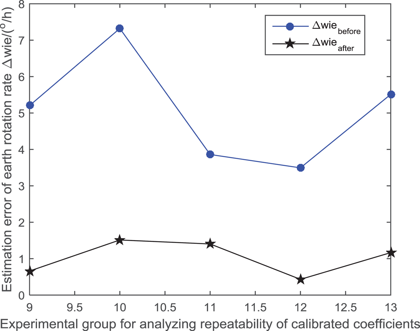
Figure 11. Comparison between Δω ie_before and Δω ie_after in five group experiments for analysing the repeatability of the coefficients calibrated.
It can be seen from the comparison results in Figure 11 that after the g-sensitivity error in the MEMS gyro output data is compensated at different start-up times using the g-sensitivity coefficients calibrated in Table 4, the output precision of the MEMS gyroscope can be improved effectively. The result indicates that the g-sensitivity error coefficients calibrated have the merit of repeatability, and thus fully verified the effectiveness of the proposed calibration method of g-sensitivity coefficients of a MEMS gyroscope.
4. CONCLUSIONS
To improve the accuracy and actual performance of high-precision MEMS gyroscopes and solve the problems in the offline calibration and compensation of g-sensitivity error, this paper proposes a new method for offline calibration and compensation for g-sensitivity coefficients. The innovation of the proposed method is manifested in the following aspects: (1) Based on the calibration model of g-sensitivity coefficients in a MEMS gyroscope, the Newton iteration and least squares methods are used for the fitting of g-sensitivity error coefficients. (2) On the basis of this theoretical analysis, the (8 + N)-position calibration scheme is designed, the MEMS gyroscope and accelerometer data collected are smoothed, and the influence of random noise on g-sensitivity coefficients calibration is eliminated. At the same time, the experimental data in the first eight symmetrical positions can effectively calibrate and compensate the triaxial bias of the MEMS gyroscope, thus offsetting its influence on the g-sensitivity coefficients calibration. (3) The proposed calibration method does not require a high-precision turntable or centrifuge and only uses a cube model, on which the MEMS gyroscope can be installed, to calibrate the g-sensitivity error at multiple positions. The calibration cost is low and the calibration process is fast and simple.
The method proposed in this paper has been verified effectively in many groups of experimental data in the high-performance STIM300 MEMS IMU system. The experimental results show that the proposed method can conduct effective offline calibration for g-sensitivity error coefficients, and the calibrated coefficients have some stability and repeatability. After the compensation of g-sensitivity error coefficients, the output precision of a high-performance MEMS gyroscope can be effectively improved.
With the continuous improvement and upgrade of manufacturing process of MEMS gyroscopes, both the stability and repeatability of g-sensitivity error coefficients are constantly improved, although the g-sensitivity error problem still exists in MEMS gyroscopes due to the principles of the MEMS gyroscopes. As a result, from the perspective of improving both precision and performance of a MEMS gyroscope, g-sensitivity error offline calibration and compensation of MEMS gyroscopes has become increasingly important.
5. FINANCIAL SUPPORT
This work was partially supported by the National Natural Science Foundation of China (Grant No. 61673208, 61533008, 61533009, 61374115), advanced research project of the Ministry of army equipment development in 13th Five-Year (30102080101), the “333 project” in Jiangsu Province (Grant No. BRA2016405), the Scientific Research Foundation for the Selected Returned Overseas Chinese Scholars(Grant No. 2016), the peak of six personnel in Jiangsu Province (Grant No. 2013-JY-013), the Aeronautic Science Foundation of China (Grant No. 20165552043, 20165852052), the Fundamental Research Funds for the Central Universities (Grant No. NZ2017001, NZ2016104, NS2017016, NP2017209), Foundation of Jiangsu Key Laboratory “Internet of Things and Control Technologies” & the Priority Academic Program Development of Jiangsu Higher Education Institutions and Jiangsu Innovation Program for Graduate Education (Grant No. CXLX13_156).