


1. INTRODUCTION
During the successfully conducted Mars exploration missions, reliance has been placed on Earth-based radiometric measurements to determine the orbit of the spacecraft (Schratz et al., Reference Schratz, Soriano, Ilott, Shidner, Chen and Bruvold2014). To fulfil pinpoint landing, the top priority is to deliver the spacecraft to the calculated atmosphere entry interface (Martinmur et al., Reference Martinmur, Kruizinga, Burkhart, Abilleira, Wong and Kangas2014). Hitherto, dependence has been on intensively conducted measurements, such as Doppler, Direct-to-Earth X-band link and Delta Differential One-way Range (ΔDOR) to predict the trajectory of the spacecraft a couple of weeks before entry (Schratz et al., Reference Schratz, Soriano, Ilott, Shidner, Chen and Bruvold2014; Quadrelli et al., Reference Quadrelli, Wood, Riedel, McHenry, Aung, Cangahuala, Volpe, Beauchamp and Cutts2015). However, accurate knowledge of the real-time state cannot be obtained because of the time delay. As a result, real-time control of the spacecraft cannot be realised (Dutta and Braun, Reference Dutta and Braun2014). Hence, autonomous orbit determination is necessary for precise control and guidance in Mars exploration.
As the abilities of small satellites have become increasingly versatile (Alfriend et al., Reference Alfriend, Vadali, Gurfil, How and Breger2009), formation flying spacecraft have been used to fulfil autonomous navigation. The advantages of using formation flying spacecraft include reducing the size of the spacecraft; reducing costs, increasing flexibility and offering a more robust navigation solution (Ning et al., Reference Ning, Avendano and Mortari2011). Markley (Reference Markley1984) initially proposed the method to determine the orbits of the two spacecraft formation flying in low Earth orbits. Psiaki (Reference Psiaki2011) applied this method to estimate the gravitational constant and J2 term of the moon. Yang presented an autonomous navigation method for a spacecraft formation flying in the proximity of an asteroid, on board optical devices and a LIDAR (Light Detection And Ranging) were used to estimate the relative position and velocity of the formation with respect to the asteroid (Yang et al., Reference Yang, Vetrisano, Vasile and Zhang2016). Maessen and Gill (Reference Maessen and Gill2012) proposed a method to estimate the relative state of the formation flying spacecraft using relative range measurements.
Observability analysis is inevitable in designing a system using formation flying spacecraft, because we cannot achieve satisfactory state estimation when the system is unobservable. Almost all systems are nonlinear in dynamics and nonlinear measurements are also widely exploited to realise autonomous navigation (Wang et al., Reference Wang and Zheng2016; Wang and Zheng, Reference Wang, Zheng, An, Sun and Li2014; Liu et al., Reference Liu, Wei and Jin2017). Considering the observability analysis methods, two approaches have been used to attack the observability of nonlinear systems (Wu et al., Reference Wu, Zhang, Wu, Hu and Hu2012). The first one uses differential geometrical theory to obtain the observability matrix. The system is said to be locally weakly observable if the full-rank condition is satisfied (Anguelova, Reference Anguelova2007; Hermann and Krener, Reference Hermann and Krener1977). However, Lie derivatives should be calculated, which ask for heavy computation for high dimensional systems. The second method turns to the Piecewise Constant (PWCS) assumption and calculating the observability matrix for the linearized system (Goshen-Meskin and Bar-Itzhack, Reference Goshen-Meskin and Bar-Itzhack1992a; Reference Goshen-Meskin and Bar-Itzhack1992b; Bemporad et al., Reference Bemporad, Ferrari-Trecate and Morari2000). Other approximate methods were also developed by researchers (Yim et al., Reference Yim, Crassidis and Junkins2004; Hill and Born, Reference Hill and Born2007). Yu et al. (Reference Yu, Cui and Zhu2015) proposed a method based on the quadratic approximation of Lie derivatives, and the condition number of the observability matrix was chosen as the performance index. Nevertheless, the approximation may induce uncertainty to the observability analysis.
The purpose of this paper is to fulfil Mars autonomous navigation using formation flying spacecraft. The top priority is to find the optimal configuration design parameters to enhance the system's observability. The methods mentioned above can only provide an index to evaluate the configuration rather than directly giving the optimal parameters. In view of this shortcoming, an analytical approach is proposed to directly find the optimal configuration. The parameters are optimally found by solving the constrained optimisation problem. When the second deputy is added into the formation, the parameters are also optimally solved. We also provide a novel explanation for the system design result from the perspective of the Fisher information theory. In simulation, the extended Kalman filter is applied to estimate the state. When there is one deputy, the position determination accuracy can be within 10 m and the velocity accuracy can be within 0·01 m/s. Furthermore, when another deputy is added, the accuracies are significantly enhanced.
The rest of the paper is organised as follows. Section 2 gives the method to design the spacecraft formation. In Section 3, we investigate the observability when there is one deputy in the formation. When another deputy is added, the observability is optimised in Section 4. In Section 5, the navigation simulation is conducted using the Extended Kalman Filter (EKF). Section 6 concludes this paper.
2. FORMATION CONFIGURATION DESIGN
2.1. Coordinate systems
Two coordinate systems are involved in this paper. The Mars J2000·0 frame is used to describe the absolute motion of formation flying spacecraft when orbiting around Mars. The origin of this frame lies in the centre of Mars, the X I axis points to the vernal equinox, the Z I axis points to the north pole of the Mars, and the Y I axis completes this right-handed system. The relative motion is described in the Local-Vertical Local-Horizontal (LVLH) frame placed at the mass centre of the chief, in which the x directs radially outwards from the chief, z is normal to the orbit plane and y completes the frame. The two types of frame are depicted in Figure 1. We assume that the measurement frame coincides with the body frame and the body frame is aligned to the LVLH frame.
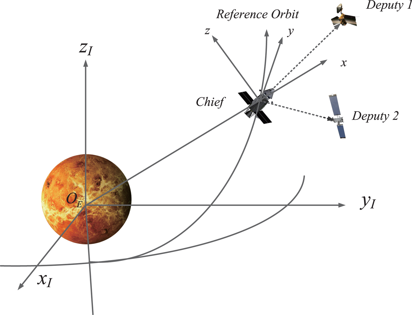
Figure 1. Coordinates and formation flying spacecraft.
2.2. Formation configuration design
The formation configuration is designed using the relative orbit elements. The Keplerian elements are defined as the semi-major axis a, eccentricity e, inclination i, right ascension of ascending node Ω, argument of perigee ω, and mean argument of latitude u. In Equation (1), five description parameters
 $\{p, s, \alpha, \theta, l\}$
are used to determine the relative motion in the LVLH frame (Zeng et al., Reference Zeng, Hu and Yao2012; Hu et al., Reference Hu, Zeng and Song2013; Ou et al., Reference Ou, Zhang and Xing2016). Based on the orbit elements of the chief, the relative orbit elements are obtained with these parameters.
$\{p, s, \alpha, \theta, l\}$
are used to determine the relative motion in the LVLH frame (Zeng et al., Reference Zeng, Hu and Yao2012; Hu et al., Reference Hu, Zeng and Song2013; Ou et al., Reference Ou, Zhang and Xing2016). Based on the orbit elements of the chief, the relative orbit elements are obtained with these parameters.
 $$\left\{ \matrix{ x = -p \,\cos (u - \theta) \hfill \cr y = 2 p \,\sin (u - \theta) + l \cr z = s \,\sin (u - \varphi) \hfill } \right.$$
p = aδe determines the semi-minor axis of the in-plane ellipse, s = aδi represents the cross-track magnitude in the relative frame, θ is the initial phase angle of the in-plane motion and ϕ is the initial phase angle of the cross-track motion. l represents the along-track offset which is set to be zero in this paper, u=nt describes the mean motion and n is the orbit angular velocity. Note that the phase angle difference
 $\alpha = \theta - \phi$
determines the spatial orientation of the relative motion in LVLH. These parameters are depicted in Figure 2.
$\alpha = \theta - \phi$
determines the spatial orientation of the relative motion in LVLH. These parameters are depicted in Figure 2.
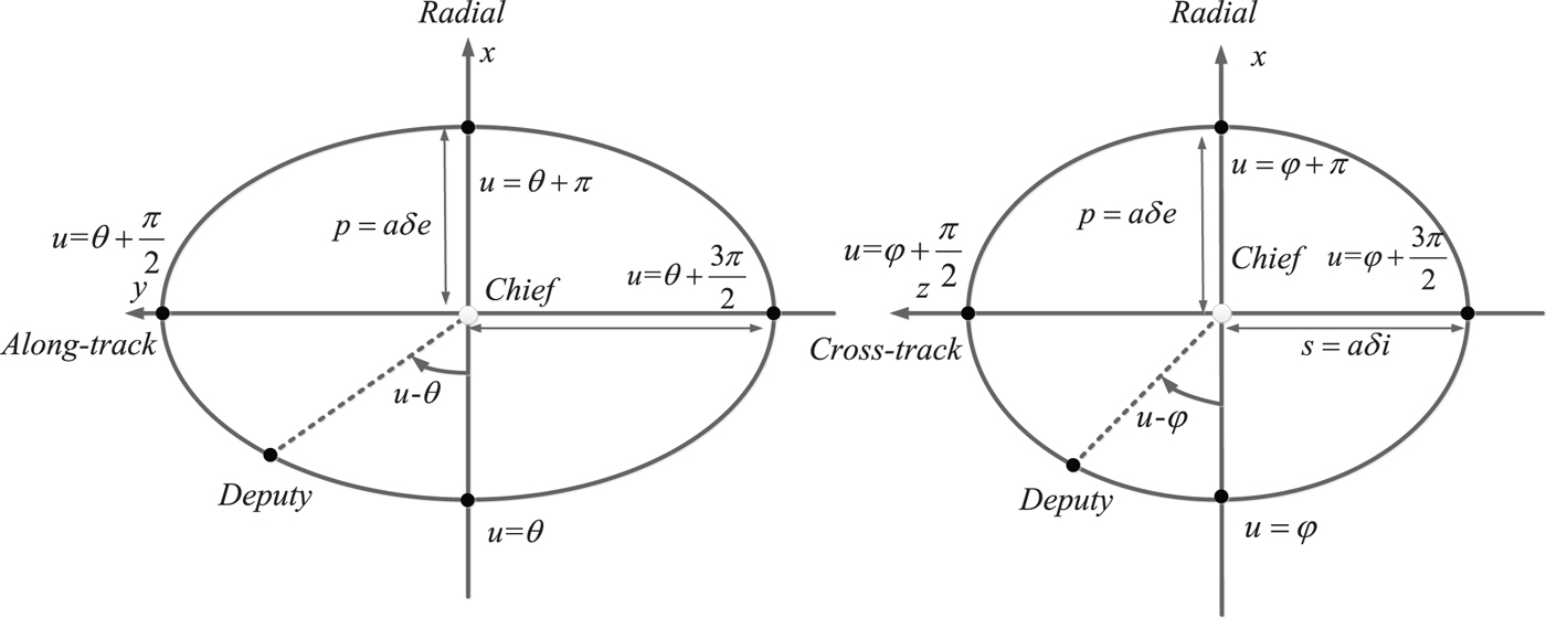
Figure 2. Parameters in relative motion frame.
3. ONE-DEPUTY FORMATION NAVIGATION SCENARIO
3.1. Nonlinear observability analysis with Lie algebra
Considering the observability analysis for nonlinear systems, differential geometrical theory and Lie algebra have received considerable attention. However, researchers are impeded by the burdensome computation of Lie derivatives when dealing with high dimensional nonlinear systems. In this section, we consider the nonlinear dynamical systems in the form
 $$\Sigma\,{:} \left\{ \matrix{ {\bi x} = {\bi f}\!({\bi x}) \cr {\bi y} = {\bi h}({\bi x}) } \right.$$
The dynamical system is corrected by adding the dot on x
 $$\Sigma\,{:} \left\{ \matrix{ \dot{{\bi x}} = {\bi f}\!({\bi x} ) \cr {\bi y} = {\bi h} ({\bi x} ) } \right.$$
Where
 ${\bi x} \in {\open R}^{n}$
denotes the n-dimensional state vector, and
${\bi x} \in {\open R}^{n}$
denotes the n-dimensional state vector, and
 ${\bi y} \in {\open R}^{m}$
denotes the m-dimensional measurement vector.
f
(
x
) refers to the dynamical function and
h
(
x
) is the measurement function.
${\bi y} \in {\open R}^{m}$
denotes the m-dimensional measurement vector.
f
(
x
) refers to the dynamical function and
h
(
x
) is the measurement function.
In order to acquire the observability matrix, theoretically, (n − 1)th-order Lie derivatives should be computed for a n-dimensional dynamical system. The (k + 1)th-order Lie derivative can be recursively computed from the kth-order Lie derivative with respect to the state equation f ( x ) as below
 $$L_f^{k + 1} {\bi h} ({\bi x}) = {\partial\lpar L_f^k {\bi h}({\bi x}) \rpar \over \partial {\bi x}} {\bi f}({\bi x})$$
Particularly, the 0th-order Lie derivative is
 $$L_f^0 {\bi h} ({\bi x}) = {\bi h} ({\bi x})$$
Then, the nonlinear observability matrix is expressed as
 $${\bi O} ({\bi x}) = \lsqb \left( d{\bi h}({\bi x}) \right)^T \left( dL_f^1 {\bi h}({\bi x}) \right)^T \cdots \lpar dL_f^{n-1} {\bi h}({\bi x}) \rpar^T \rsqb ^T$$
where the differential of
 $L_{f}^{k} {\bi h} ({\bi x})$
with respect to the state is defined as
$L_{f}^{k} {\bi h} ({\bi x})$
with respect to the state is defined as
 $$dL_f^k {\bi h} ({\bi x}) = {\partial L_f^k {\bi h} ({\bi x}) \over \partial {\bi x}}$$
If the observability matrix satisfies the full-rank condition, the system is said to be locally weakly observable (Kassas and Humphreys, Reference Kassas and Humphreys2014).
In contrast with the nonlinear observability analysis, the linearized approach is based on the piecewise constant assumption. Considering the same dynamical system, the linearized observability matrix is computed as (Chen and Xu, Reference Chen and Xu2010).
 $${\bi O}_n ({\bi x}) = \left[ \matrix{ {\bi H}\lpar {\bi x}_k \rpar \cr {\bi H}\lpar {\bi x}_{k+1} \rpar {\bi \Phi} \lpar {\bi x}_k \rpar \cr {\bi H}\lpar {\bi x}_{k+2} \rpar {\bi \Phi} \lpar {\bi x}_{k+1} \rpar {\bi \Phi} \lpar {\bi x}_k \rpar \cr \vdots \cr {\bi H}\lpar {\bi x}_{k+(n-1)} \rpar {\bi \Phi} \lpar {\bi x}_{k+(n-2)} \rpar \cdots {\bi \Phi} \lpar {\bi x}_k \rpar } \right]$$
where the measurement matrix H and state transition matrix Φ are defined as
 $${\bi H} = {\partial {\bi h} ({\bi x}) \over \partial {\bi x}}$$
 $${\bi \Phi} = {\bi I} + {\partial {\bi f} ({\bi x}) \over \partial {\bi x}}{\cdot}T$$
where T is the update step.
3.2. One-deputy observability optimisation
As is shown in Figure 3, the relative line-of-sight vectors can be measured using LIDAR and other optical devices. Based on the attitude sensors, the inertial line-of-sight vector measurements can be obtained by transforming the relative line-of-sight measurements to the inertial frame. The orbit dynamical equation and measurement equation are

Figure 3. Relative measurement model.
 $$\left[\matrix{ \dot{\bi r} \cr \dot{\bi v} } \right] = \left[ \matrix{ {\bi v} \cr -\mu {\bi r}_i /\Vert r_i \Vert^3 } \right]$$
 $$\eqalign{ {\bi y} &= {\bi r}_2 - {\bi r}_1 \cr &= {\bi C}_b^I \left[ \matrix{ \rho \cos \beta \cos \gamma \cr \rho \cos \beta \sin \gamma \cr \rho \sin \beta \hfill} \right] }$$
where
 ${\bi C}_{b}^{I}$
is the attitude matrix transforming the relative measurements to the inertial frame, ρ is the relative range, β is the elevation angle and γ is the azimuth angle.
${\bi C}_{b}^{I}$
is the attitude matrix transforming the relative measurements to the inertial frame, ρ is the relative range, β is the elevation angle and γ is the azimuth angle.
Theoretically, n − 1 order Lie derivatives should be calculated and concatenated to obtain the observability matrix (Anguelova, Reference Anguelova2007). Based on the analysis from Psiaki (Reference Psiaki2011), in order to find the conditions that make the system unobservable, we only need to calculate the matrix to be square since the null space of O k ( x ) x = 0 is necessarily contained in the null space of O j ( x ) x = 0 for all j < k. Inspired by this conclusion, the square-form nonlinear observability matrix for the one-deputy system is computed as below
 $${\bi O} ({\bi x}) = d \left[\matrix{ {\bi h}({\bi x}) \cr {\bi v}_{1} - {\bi v}_{2} \cr {\bi g}_{1} - {\bi g}_{2} \cr {\bi G}_{1} {\bi v}_{1} - {\bi G}_{2} {\bi v}_{2} } \right]= \left[\matrix{ {\bi I} & {\bi 0} &-{\bi I} &{\bi 0}\cr {\bi 0} & {\bi I} &{\bi 0} &-{\bi I}\cr {\bi G}_1 & {\bi 0} &-{\bi G}_2 &{\bi 0}\cr \dot{{\bi G}}_1 & {\bi G}_1 &\dot{{\bi G}}_2 &-{\bi G}_2 } \right]$$
where the gravity gradient tensor G i and its differentials with respect to the states Ġ i are
 $${\bi G}_i = {\mu \over \Vert r_i \Vert ^3} \lpar 3{\bi r}_i {\bi r}_i^T - {\bi I} \rpar $$
 $$\dot{\bi G}_i = {\mu \over \Vert r_i \Vert ^4} \lsqb {\bi v}_i {\bi r}_i^T + {\bi r}_i {\bi v}_i^T - \lpar {\bi r}_i^T {\bi v}_i \rpar \lpar 5{\bi r}_i {\bi r}_i^T - {\bi I} \rpar \rsqb $$
Generally, we tend to find the most observable configurations directly. Nevertheless, methods available now just outline the unobservable cases which should be avoided. Through close observation of the elements of the observability matrix, we conclude that the observability is determined by the linear correlation between columns or rows. Intuitively, when these columns and rows of the observability matrix are weakly correlated, the matrix is more positive definite. Therefore, the linear correlation between the columns or rows can be exploited to enhance the observability.
In Equation (11), expanding the difference between
G
1 and
G
2 to enhance the matrix's positive definiteness is straightforward. In the physical sense, we are enlarging the disparity of the two spacecraft's gravity gradient tensors. Now, the Frobenius norm of matrix difference is
 $\Vert {\bi G}_{1} - {\bi G}_{2} \Vert _{F}$
, defined below, since this norm can reflect the matrix difference to the maximal extent (Böttcher and Wenzel, Reference Böttcher and Wenzel2008).
$\Vert {\bi G}_{1} - {\bi G}_{2} \Vert _{F}$
, defined below, since this norm can reflect the matrix difference to the maximal extent (Böttcher and Wenzel, Reference Böttcher and Wenzel2008).
 $$\Vert A \Vert _F = \left(\sum_{i = 1}^{m} \sum_{j = 1}^{n} \vert a_{ij} \vert^2 \right)^{1 \over 2}$$
The positions of the chief and the deputy can be expressed in the LVLH frame as below
 $${\bi r}_1 = \lsqb r_1, 0, 0 \rsqb ^T$$
 $${\bi r}_2 = \lsqb r_2 + x, y, z \rsqb ^T$$
r 1 is the distance from the chief to the centre of Mars, and [x, y, z] T is the relative position vector in the LVLH frame. The difference of gravity gradient tensor is calculated as
 $$\eqalign{ {\bi G}_1 - {\bi G}_2 &= {\mu \over \Vert {\bi r}_1 \Vert ^3} \lpar 3 {\bi r}_1 {\bi r}_1^T - {\bi I} \rpar - {\mu \over \Vert {\bi r}_2 \Vert ^3} \lpar 3 {\bi r}_2 {\bi r}_2^T - {\bi I} \rpar \cr &= {3\mu \over \Vert {\bi r}_1 \Vert ^3} {\bi r}_1 {\bi r}_1^T - {3\mu \over \Vert {\bi r}_2 \Vert ^3} {\bi r}_2 {\bi r}_2^T + \left({\mu \over \Vert {\bi r}_1 \Vert^3} - {\mu \over \Vert {\bi r}_2 \Vert^3} \right) {\bi I} \cr &={3\mu \over \Vert {\bi r}_1 \Vert ^3} \left({\bi r}_1 {\bi r}_1^T - {\Vert {\bi r}_1 \Vert^3 \over \lpar \lpar r_1 + x \rpar^2 + y^2 +z^2 \rpar^{3 \over 2}} - {\bi r}_2 {\bi r}_2^T\right) + \left({\mu \over \Vert {\bi r}_1 \Vert^3} - {\mu \over \Vert {\bi r}_2 \Vert^3} \right) {\bi I} \cr &\approx {3\mu \over \Vert {\bi r}_1 \Vert ^3} \left({\bi r}_1 {\bi r}_1^T - \left(1 - {3x \over r_1} \right) {\bi r}_2 {\bi r}_2^T \right) + \left({\mu \over \Vert {\bi r}_1 \Vert^3} - {\mu \over \Vert {\bi r}_2 \Vert^3} \right) {\bi I} \cr &\approx {3\mu \over \Vert {\bi r}_1 \Vert ^3} \lpar {\bi r}_1 {\bi r}_1^T - {\bi r}_2 {\bi r}_2^T \rpar }$$
where the minutiae are omitted, then we turn to the new object
 $${\bi r}_2 {\bi r}_2^T - {\bi r}_1 {\bi r}_1^T =\left(\matrix{ 2r_1 x + x^2 &\lpar r_1 + x \rpar y &\lpar r_1 + x \rpar z \cr \lpar r_1 + x \rpar y & y^2 & yz \cr \lpar r_1 + x \rpar z & yz & z^2 } \right)$$
The Frobenius norm of this matrix is computed as
 $$\eqalign{ &\Vert {\bi r}_2 {\bi r}_2^T - {\bi r}_1 {\bi r}_1^T \Vert _F \cr &= \sqrt{\lpar x^2 + 2r_1 x \rpar ^2 + 2\lpar y \lpar x + r_1 \rpar \rpar ^2 + 2\lpar z \lpar x + r_1 \rpar \rpar ^2 + 2y^2 z^2 + y^4 + z^4} }$$
Then the final performance index is chosen as
 $$J = \lpar 2r_1 x + x^2 \rpar ^2 + 2y^2 \lpar r_1 + x \rpar ^2 + 2z^2 \lpar r_1 + x \rpar ^2 + y^4 + 2y^2 z^2 + z^4$$
For a formation system with only one deputy, the description parameters should be optimised to elevate the system's observability. Among the five parameters, the impact of
r
1 has been investigated thoroughly by other researchers and θ does not influence the spatial configuration, l is set to zero in this paper. Three parameters
 $\{p, s, \alpha\}$
are left to be optimised.
$\{p, s, \alpha\}$
are left to be optimised.
According to Equations (14) and (15) and Equation (1), we assume that the initial in-plane phase angle is 0 when t=0; the position vectors can be rewritten as
 $$\left\{ \matrix{ {\bi r}_1 = \lsqb r_1, 0, 0 \rsqb^{T} \hfill \cr {\bi r}_2 = \lsqb r_1 - p, 0, -s \sin \alpha \rsqb^T } \right.$$
The performance index is computed as
 $$J = \lpar -2r_1 p + p^2 \rpar ^2 + 2s^2 \lpar r_1 - p \rpar ^2 \sin^2 \alpha + s^4 \sin^4 \alpha$$
With the restriction, the constrained optimisation problem can be stated as
 $$\eqalign{ & min - J (\alpha, p, s) \cr & S.t: \left\{ \matrix{ 0 < \alpha \le 2\pi \cr 0 < p \le q_1 \cr 0 < s \le q_2 } \right. }$$
To handle the preceding problem, the Lagrange function is defined as
 $$L \lpar \alpha, p, s, \gamma_1, \gamma_2, \gamma_3 \rpar = -J - \gamma_1 (2\pi - \alpha) - \gamma_2 \lpar q_1 - p \rpar - \gamma_3 \lpar q_2 - s \rpar $$
Where q
1, q
2 determine the size of the relative motion trajectory, and γ1, γ2, γ3 are the Lagrange multipliers. The solution of this problem is
 $\alpha = \pi /2, 3\pi /2, p = q_{1}, s = q_{2}$
.
$\alpha = \pi /2, 3\pi /2, p = q_{1}, s = q_{2}$
.
4. TWO-DEPUTY FORMATION NAVIGATION SCENARIO
When another deputy is added to the original navigation scheme, more parameters are involved in designing the configuration. When there are two deputies orbiting around the chief, the Lie derivatives are calculated as
 $$\eqalign{ L_f^0 {\bi h} ({\bi x}) &= {\bi h}({\bi x})=\left[ \matrix{ {\bi r}_1 - {\bi r}_2 \cr {\bi r}_1 - {\bi r}_3 } \right] \cr L_f^1 {\bi h} ({\bi x}) &= {\partial {\bi h} \lpar {\bi x}\rpar \over \partial {\bi x}} {\bi f}\!({\bi x}) \left[\matrix{ {\bi v}_1 - {\bi v}_2\cr {\bi v}_1 - {\bi v}_3 } \right] \cr L_f^2 {\bi h} ({\bi x}) &= {\partial L_f^1 {\bi h} \lpar {\bi x}\rpar \over \partial {\bi x}} {\bi f}\!({\bi x}) = \left[\matrix{ {\bi g}_1 - {\bi g}_2 \cr {\bi g}_1 - {\bi g}_3 } \right] }$$
The nonlinear observability matrix for the three-spacecraft formation is computed as
 $${\bi O} ({\bi x}) = d \left[\matrix{ {\bi h}({\bi x}) \cr {\bi v}_{1} - {\bi v}_{2} \cr {\bi v}_{1} - {\bi v}_{3} \cr {\bi g}_{1} - {\bi g}_{2} \cr {\bi g}_{1} - {\bi g}_{3} } \right]= \left[\matrix{ {\bi I} & {\bi 0} &-{\bi I} &{\bi 0} &{\bi 0} &{\bi 0}\cr {\bi I} & {\bi 0} &{\bi 0} &{\bi 0} &-{\bi I} &{\bi 0}\cr {\bi 0} & {\bi I} &{\bi 0} &-{\bi I} &{\bi 0} &{\bi 0}\cr {\bi 0} & {\bi I} &{\bi 0} &{\bi 0} &{\bi 0} &-{\bi I}\cr {\bi G}_1 & {\bi 0} &-{\bi G}_2 &{\bi 0} &{\bi 0} &{\bi 0}\cr {\bi G}_1 &{\bi 0} &{\bi 0} &{\bi 0} &-{\bi G}_3 &{\bi 0} } \right]$$
The navigation scheme is depicted in Figure 4. We also assume that the initial phase angles of the first deputy are θ1 = 0, α1 = π / 2, and the initial phase angles of the second deputy are θ2 = θ, α2 = α which will be optimised in this section. Following the previous method, the position vectors can be rewritten as

Figure 4. Two-deputy navigation scheme.
 $$\left\{ \matrix{ {\bi r}_2 = \lsqb r_1 - p, 0, -s \rsqb^T \hfill \cr {\bi r}_3 = \lsqb r_1 - p \cos \theta, 2p \sin \theta, s \sin \lpar \theta - \alpha \rpar \rsqb^T } \right.$$
Using Equation (17), the performance index is calculated as
 $$\eqalign{ J &= 16 p^4 \sin^4 \theta + \lpar \lpar r_1 - p \cos \theta \rpar^2 - \lpar r_1 - p\rpar^2 \rpar ^2 + 8\lpar p \sin \theta \lpar r_1 - p \cos \theta \rpar \rpar ^2 \cr &\quad + 2 \lpar s \sin \lpar \theta - \alpha \rpar \lpar r_1 - p \cos \theta \rpar + s \lpar r_1 - p \rpar \rpar ^2 + 8\lpar ps \sin \theta \sin \lpar \theta - \alpha \rpar \rpar ^2 \cr &\quad + \lpar s^2 - s^2 \sin^2 \lpar \theta - \alpha \rpar \rpar ^2 }$$
The constrained optimisation problem can be stated as
 $$\eqalign{ &min - J (\alpha, \theta) \cr &S.t: \left\{ \matrix{ 0 < \theta \le 2\pi \cr 0 < \alpha < 2\pi } \right. }$$
Solving this constrained optimisation problem, four solutions are obtained as follows and the details are given in the Appendix.
 $$1. \left\{ \matrix{ \alpha = {\pi \over 2} \cr \theta = \pi } \right., \quad 2. \left\{ \matrix{ \alpha = {3\pi \over 2} \cr \theta = \pi } \right.$$
 $$\eqalign{ &3. \left\{ \matrix{ \theta = \arccos t \hfill\cr t = -{-13 p^2 -3s^2 + 2 pr_1 - 2r_1^2 + \sqrt{\lpar 13 p^2 +3s^2 - 2pr_1 + 2r_1^2 \rpar^2 + 36pr_1 \lpar s^2 + 3pr_1 + 2r_1^2 \rpar } \over 18 pr_1} \cr \alpha = \theta + \pi / 2 \hfill} \right. \cr &4. \left\{ \matrix{ \theta = \Vert \arccos t \Vert \hfill\cr t = {1 \over 18 p^2 r_1} \lpar -13 p^3 - 3ps^2 + 2p^2 r_1 - 2pr_1^2 \rpar \hfill\cr \qquad - {1 \over 18 p^2 r_1} \sqrt{\lpar 13 p^3 + 3ps^2 - 2p^2 r_1 + 2p r_1^2 \rpar^2 + 36p^2 r_1 \lpar -ps^2 + 3p^2 r_1 + 2s^2 r_1 + 2pr_1^2 \rpar } \cr \alpha = \theta - \pi / 2 \hfill} \right. }$$
To find out which is the global optimal solution, we use numerical methods. In this work, the Particle Swarm Optimisation (PSO) algorithm is applied to obtain the global optimum. As is shown in Figure 5, the optimal values for θ and α reside in the neighbourhood of π and π/2. The deviations between solutions 1–2 and the results of PSO are depicted in Figure 6, in which the difference between solution 1 and the global optimum varies within 0·02%. Solutions 3–4 are compared in Figure 7 and solution 4 is approximately the same as solution 1. According to these results, the global optimal solution is
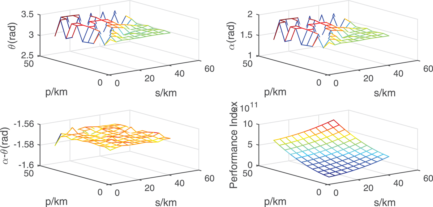
Figure 5. The results of optimal parameters using PSO.

Figure 6. The results of solution 1–2 and their deviations with PSO.

Figure 7. The results of solutions 3–4.
 $$\left\{ \matrix{ \theta = \pi \cr \alpha = {\pi \over 2} } \right.$$
Although we have obtained the optimal design parameters for the two-deputy formation system, the Fisher information theory can also give us an insightful explanation of this result. In the estimation theory, the covariance matrix of any unbiased estimator satisfies
 $${\bi C}_{\hat{\theta}} \ge {\bi I}^{-1} \lpar {\bf \theta} \rpar $$
where I ( θ ) is referred to as the Fisher information, and
 $$\lsqb {\bi I} \lpar {\bf \theta} \rpar \rsqb _{ij} = -E \left[ {\partial^2 \ln p\!\lpar {\bi x}; {\bf \theta} \rpar \over \partial {\bf \theta}_i \partial {\bf \theta}_j} \right]$$
where E denotes the expectation.
When there are N IID (Independent Identically Distributed) observations with identical probability density function p( x [n]; θ ), the overall Fisher information becomes
 $$-E \left[{\partial^2 \ln p\!\lpar {\bi x}; {\bf \theta} \rpar \over \partial {\bf \theta} \partial {\bf \theta}^T} \right] = -\sum_{n=0}^{N-1} E \left[{\partial^2 \ln p\!\lpar {\bi x} \lsqb n \rsqb ; {\bf \theta} \rpar \over \partial {\bf \theta} \partial {\bf \theta}^T}\right]$$
which is N times the single observation. Therefore, only when the observations between the chief and the two deputies are independent and identically distributed, can the navigation accuracy be doubled. Consider the problem confronted in this paper, the observations with respect to the two deputies are shown as below
 $$\eqalign{ {\bi h}_1 (k) &= {\bi C}_b^I \left[ \matrix{ \rho_1 \cos \beta_1 cos \gamma_1 \cr \rho_1 \cos \beta_1 \sin \gamma_1 \cr \rho_1 \sin \beta_1 \hfill}\right] \lpar k \rpar + {\bi v} \lpar k \rpar \cr {\bi h}_2 (k) &= {\bi C}_b^I \left[ \matrix{ \rho_2 \cos \beta_2 cos \gamma_2 \cr \rho_2 \cos \beta_2 \sin \gamma_2 \cr \rho_2 \sin \beta_2 \hfill} \right] \lpar k \rpar + {\bi v} \lpar k \rpar }$$
In view of the requirement, two observations should have the same mean in each period and thus they will have the same covariance under identical measurement noises.
 $$E\lsqb {\bi h}_1 \lpar k \rpar \rsqb = E\lsqb {\bi h}_2 \lpar k \rpar \rsqb $$
This means two measurements should have the same time history. Since the measurement information with respect to each deputy is repeated every half of the period, the measurements in each half cycle are statistically equivalent. Based on this, we obtain the following constraint that should be followed
 $$\left\{ \matrix{ \rho_1 \lpar k \rpar = \rho_2 \lpar k \rpar \hfill\cr \beta_1 \lpar k \rpar = \pm \beta_2 \lpar k \rpar \hfill\cr \gamma_1 \lpar k \rpar = \pm \gamma_2 \lpar k \rpar , \gamma_2 \lpar k \rpar + \pi } \right.$$
Obviously, the result in Equation (34) satisfies this constraint and requires that two deputies should be situated on the same trajectory and one always lags the other for half of a period.
5. NAVIGATION SIMULATION
Numerical analysis is conducted in this section to validate the above conclusions. The observability matrix is computed numerically with a Piecewise Constant (PWCS) assumption to verify the result of the theoretical analysis. For a discrete-time system as below, an EKF is designed to estimate the position and velocity of formation flying spacecraft.
 $$\left\{ \matrix{ {\bi x}_k = \phi_{k-1} \lpar {\bi x}_{k-1} \rpar + {\bi w}_{k-1} \cr {\bi y}_k = {\bi h}_{k} \lpar {\bi x}_{k} \rpar + {\bi v}_{k} \hfill} \right.$$
 ${\bi w}_{k} \sim N \lpar 0, {\bi Q}_{k} \rpar $
is the process noise and
${\bi w}_{k} \sim N \lpar 0, {\bi Q}_{k} \rpar $
is the process noise and
 ${\bi v}_{k} \sim N \lpar 0, {\bi R}_{k} \rpar $
is the measurement noise. The discrete extended Kalman filter equations are given as follows (Brown and Hwang, Reference Brown and Hwang1997)
${\bi v}_{k} \sim N \lpar 0, {\bi R}_{k} \rpar $
is the measurement noise. The discrete extended Kalman filter equations are given as follows (Brown and Hwang, Reference Brown and Hwang1997)
 $$\eqalign{ &{\bi x}_{k\vert k-1} = \phi_{k\vert k-1} \lpar {\bi x}_{k-1} \rpar \cr &{\bi y}_{k} = {\bi h}_{k} \lpar {\bi x}_{k \vert k-1} \rpar \cr &{\bi P}_{k\vert k-1} = {\bi \Phi}_{k-1} {\bi P}_{k-1} {\bi \Phi}_{k-1}^T + {\bi Q}_{k-1} \cr &{\bi K}_{k} = {\bi P}_{k \vert k-1} {\bi H}_{k}^T \lsqb {\bi H}_{k} {\bi P}_{k \vert k-1} {\bi H}_{k}^T + {\bi R}_{k} \rsqb ^{-1} \cr &{\bi x}_{k} = {\bi x}_{k \vert k-1} + {\bi K}_{k} \lpar {\bi y}_{k} - {\bi y}_{k} \rpar \cr &{\bi P}_{k} = \lpar {\bi I} - {\bi K}_{k} {\bi H}_k \rpar {\bi P}_{k\vert k-1} }$$
5.1. One-deputy formation navigation performance
When there is one deputy around the chief, at first, we investigate the relationship between the relative position and the observability. The description parameters are randomly set as {p = 10 km, s = 20 km,
 $\alpha = \pi /2$
, θ=0}, and the initial orbit elements of the chief and the deputy are given in Table 1.
$\alpha = \pi /2$
, θ=0}, and the initial orbit elements of the chief and the deputy are given in Table 1.
Table 1. Initial orbital elements of two spacecraft.

According to the orbit elements, a numerical method is used to compute the observability matrix using Equation (7), in which the measurement matrix and the state transition matrix are
 $${\bi H} = \left[\matrix{ -{\bi I} &{\bi 0} &{\bi I} &{\bi 0} } \right]$$
 $${\bi \Phi} = {\bi I}+{\bi A} \cdot T$$
where A is the Jacobian matrix
 $${\bi A} = \left[\matrix{ {\bi 0} & {\bi I} &{\bi 0} &{\bi 0}\cr {\bi G}_1 & {\bi 0} &{\bi 0} &{\bi 0}\cr {\bi 0} & {\bi 0} &{\bi 0} &{\bi I}\cr \dot{{\bi 0}} & {\bi 0} &{{\bi G}}_2 &{\bi 0} } \right]$$
The condition number is shown in Figure 8, and Figure 9 illustrates the performance index in Equation (19). According to Figures 8 and 9, the performance index synchronously changes with the condition number, and the performance index reaches its nadir when the condition number reaches the apogee. This result also reveals that the system's observability is time-variant. Particularly, the most observable place lies at the point when the deputy's out-of-plane magnitude reaches the maximum. At this time, the deputy is far away from the reference orbit plane and the gravity gradient tensor difference becomes the most considerable.

Figure 8. The variation of condition number with time.

Figure 9. The variation of performance index with the time.
Now we examine the influence of p, s when α = π/2; orbit elements for the deputy are re-calculated with various p and s. Also, we observe the effect of α with p and s settled in Equation (21). The results are depicted in Figure 10, which reveals that the effects of p and s are more dominant than α. The variation of the performance index invoked by α is nearly one magnitude less than that caused by the variation of p and s. Moreover, when α = π/2; and 3π/2 the observability becomes the best.
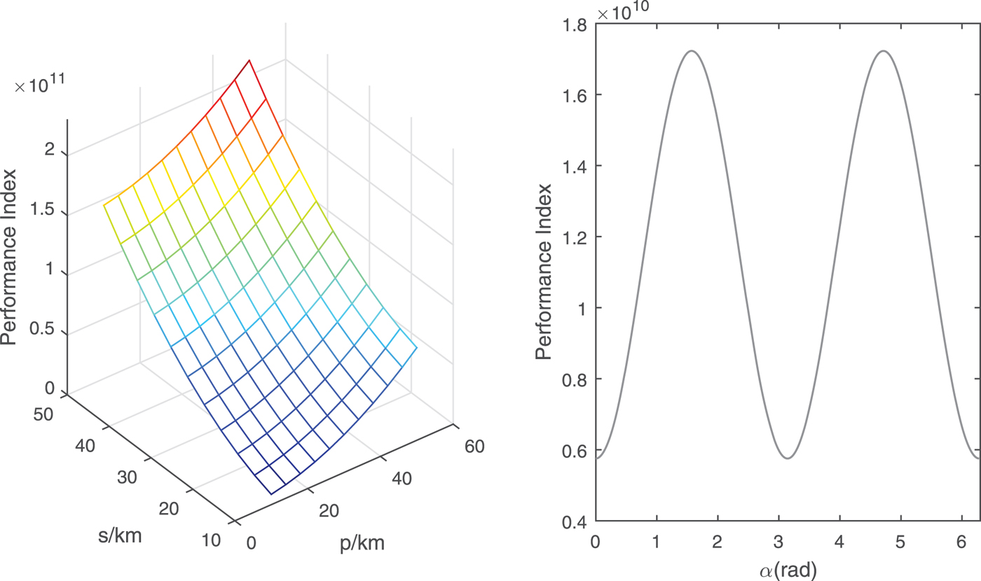
Figure 10. The variation of the performance index with p, s,α.
The analysis above has demonstrated the validity of the analytical solutions. In practice, the improvement in navigational accuracy is the most straightforward way to evaluate the performance of any proposed navigation system. Therefore, an extended Kalman filter is applied here and the navigation accuracies are compared. The parameters in the filter are presented in Table 2.
Table 2. Filter parameters setting (Unit:km2).

The dynamical model with J 2 perturbation is considered in the filter, and the filtering period is ten seconds. Figure 11 shows that the effects of p and s are considerable in improving the navigation accuracy, while the effect of α is limited. This result coincides with the conclusion from Figure 10.
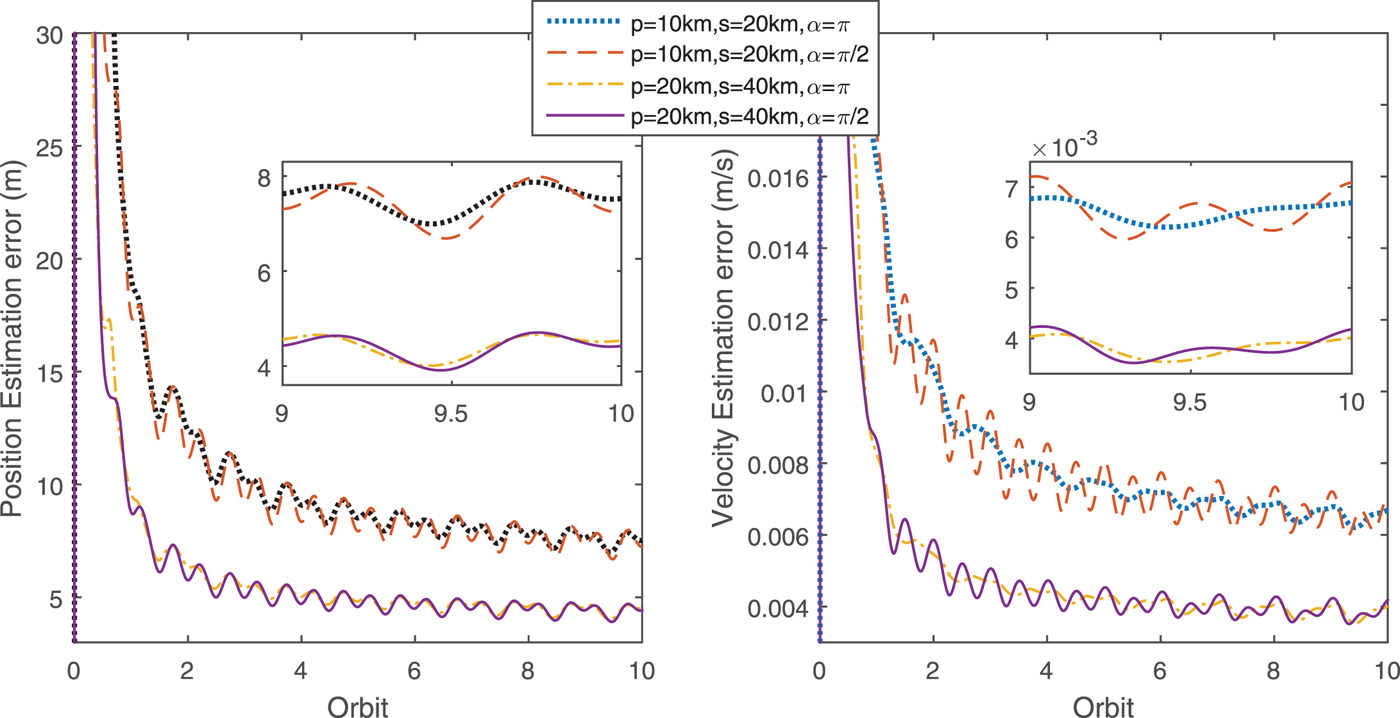
Figure 11. The influence of p, s,α on position estimation accuracy (1σ).
5.2. Two-deputy formation navigation performance
In this section, the parameters used in the extended Kalman filter are identical to those in Table 2. We assume that the initial phase angles for the first deputy are α1 = π/2, θ1=0 and α2 = α and θ2 = θ for the second deputy. Four cases are compared in Figure 12, the result confirms that the influence of α is quite limited.
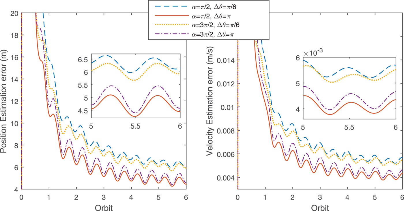
Figure 12. The position estimation accuracy with different α, Δ θ (1σ).
The design parameters for the second deputy are set as α2 = π/2, θ2 = π and orbit elements of this formation are listed in Table 3. The position and velocity estimation results are displayed in Figures 13 and 14, in which the position determination accuracy is within 10 m and the velocity accuracy is less than 0·01 m/s. Note that the parameters obtained through optimisation are the global optimum over the whole time interval. The reason is that we have optimised the relative in-plane phase angle difference Δ θ between the two deputies. The angle α of the second deputy is invariant when flying around the chief. Finally, the navigation performance of two navigation scenarios are compared. As illustrated in Figure 15, the navigation errors using two deputies are half those using only one deputy. This result encourages us to add another auxiliary micro-spacecraft to expedite convergence and enhance the navigation accuracy. Additionally, more auxiliary deputies can make the system robust and allow for the malfunction of one deputy.

Figure 13. The position estimation error with α=π/2, Δ θ=π.
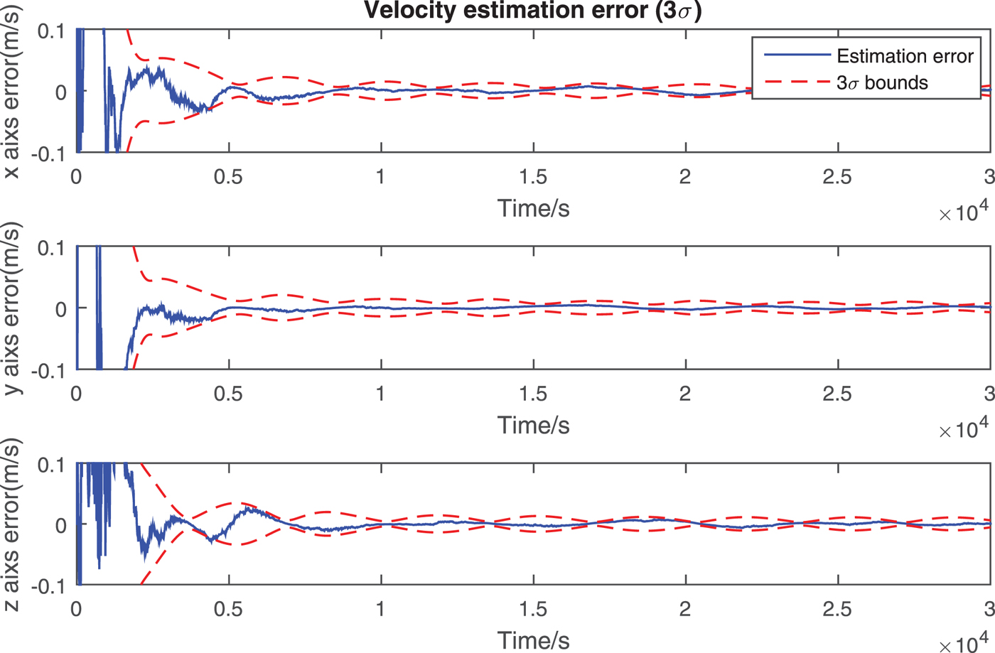
Figure 14. The velocity estimation error with α=π/2, Δ θ=π.
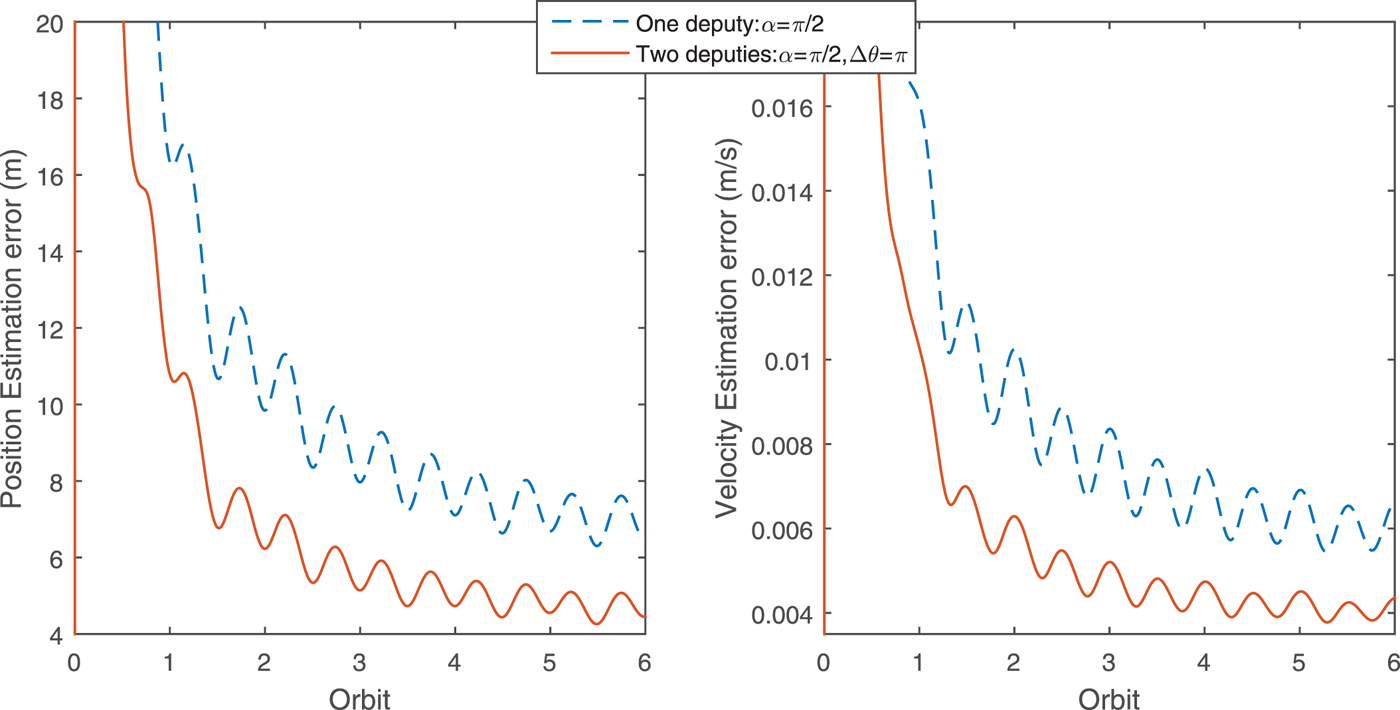
Figure 15. The position estimation accuracy comparison (1σ).
Table 3. Orbit elements of three spacecraft.

6. CONCLUSION
In this paper, an observability-based approach was proposed to improve a Mars navigation system using formation flying spacecraft. Inspired by the positive definiteness of the observability matrix that was calculated with a differential geometrical approach, the gravity gradient tensor difference was finally selected as the performance index to optimise the observability. The solutions were obtained by analytically solving the constrained optimisation problem. Moreover, the numerical observability analysis based on piecewise constant assumption was conducted to examine the validity of these analytical solutions. Finally, the feasibility and correctness of these results were demonstrated by the navigation simulations. These results reveal that the system's observability is severely influenced by the magnitude of motion in the in-track and cross-track directions. When there is only one deputy surrounding the chief, observability is mainly determined by the magnitude of the relative distance. The observability varies with time and is the best when the deputy lies far away from the chief's orbit plane. When the second deputy is added, the observability will be enhanced and the best situation happens when the two deputies are situated in the same relative orbit and one deputy always lags the other for half a period. Future work may include combining the performance index with the orbit elements, which seems to be more appropriate in describing the relative motion.
ACKNOWLEDGEMENTS
This work is supported by the Major Program of National Natural Science Foundation of China under Grant Numbers 61690210 and 61690213.
APPENDIX
When p and s are in the same magnitude, α is trivial in affecting the observability and the navigation performance. As a result, we only constrain the domain of θ in this work for simplicity. This problem can be expressed as Kuhn-Tucker conditions as follows
 $$\left\{ \matrix{ -{\partial J \lpar \alpha, p, s \rpar \over \partial \theta} + \gamma_1 = 0 \hfill\cr {\partial J \lpar \alpha, p, s \rpar \over \partial \alpha} = 0 \hfill\cr \gamma_1 \lpar 2\pi - \theta \rpar = 0 \hfill\cr \gamma_1 \ge 0 \hfill} \right.$$
Two cases should be discussed to simplify the solution.
-
1. When γ1=0, the constraints are reduced to
 $$\left\{ \matrix{ {\partial J \lpar \alpha, p, s \rpar \over \partial \theta} = 0 \cr {\partial J \lpar \alpha, p, s \rpar \over \partial \alpha} = 0 } \right.$$
which is an unconstrained optimisation problem, now we are going to solve this equation
 $$\left\{ \eqalign{ &16 p^4 \sin^3 \theta \cos \theta + 4 p^3 \sin^3 \theta\!\lpar r_1 - p \cos \theta \rpar + 4p^2 \sin \theta \cos \theta\!\lpar r_1 - p \cos \theta \rpar^2 \cr &+\,p^2 \sin \theta\!\lpar \cos \theta - 1 \rpar \lpar r_1 - p \cos \theta \rpar \lpar p \cos \theta + p -2r_1\rpar -2p^2 s^2 \sin^2 \theta \sin^2 \theta \sin 2\!\lpar \alpha - \theta \rpar \cr &+\,s \lpar \sin (\alpha- \theta) \lpar p \cos \theta - r_1 \rpar -p+r_1\rpar \lpar r_1 s \cos \lpar \alpha-\theta \rpar ps \cos\!\lpar \alpha - 2\theta \rpar \rpar \cr &+\,2p^2 s^2 \sin 2\theta \sin \theta \sin^2\!\lpar \alpha - \theta \rpar + s^4 \sin\!\lpar \alpha - \theta \rpar \cos^3\!\lpar \alpha - \theta \rpar = 0 \cr &4s \cos \lpar \alpha - \theta \rpar \left(\matrix{ 4 p^2 s \sin^2 \theta \sin \lpar \alpha - \theta \rpar - s^3 \sin\!\lpar \alpha - \theta \rpar \cos^2\!\lpar \alpha - \theta \rpar \cr -s\!\lpar r_1 - p \cos \theta \rpar \lpar \sin\!\lpar \alpha - \theta \rpar \lpar p \cos \theta - r_1 \rpar - p + r_1 \rpar } \right) = 0 } \right.$$
At first, we begin to discuss which part of the second equation is equal to zero.
(a) If
 $\cos \lpar \alpha - \theta \rpar = 0, \alpha - \theta = \pi/2, -\pi/2, 3\pi/2, -3\pi/2$
. In this case, we also need to discuss this two situations as follows
$\cos \lpar \alpha - \theta \rpar = 0, \alpha - \theta = \pi/2, -\pi/2, 3\pi/2, -3\pi/2$
. In this case, we also need to discuss this two situations as follows
 $$\left\{ \matrix{ \sin\!\lpar \alpha - \theta \rpar = 1 \hfill\cr \sin\!\lpar \alpha - \theta \rpar = -1 } \right.$$
i. When in the case of
 $\sin (\alpha - \theta) = 1, \alpha - \theta = \pi/2, -3\pi/2$
. Substitute
$\sin (\alpha - \theta) = 1, \alpha - \theta = \pi/2, -3\pi/2$
. Substitute
 $\cos(\alpha - \theta) = 0$
and
$\cos(\alpha - \theta) = 0$
and
 $\sin (\alpha - \theta ) = 1$
into
$\sin (\alpha - \theta ) = 1$
into
 ${\partial J (\alpha,\, p,\, s) \over \partial \alpha} = 0$
.
${\partial J (\alpha,\, p,\, s) \over \partial \alpha} = 0$
.
 $$p^2 \sin \theta\!\left( \eqalign{ &-9 p^2 \cos 3\theta + \cos \theta\!\lpar 25 p^2 + 12s^2 \rpar - 2pr_1\!\lpar 4\cos \theta + 9\cos 2\theta + 3 \rpar \cr &+\,8r_1^2 \lpar \cos \theta + 1 \rpar + 4s^2 } \right) = 0$$
Since
 $0 < \alpha < \pi$
,
$0 < \alpha < \pi$
,
 $0< \theta < 2 \pi$
, we obtain the solution.
$0< \theta < 2 \pi$
, we obtain the solution.
 $$\left\{ \matrix{ \alpha = {3\pi \over 2} \cr \theta = \pi \hfill} \right.$$
Another solution is solved by letting the polynomial in the bracket equal to zero. It worth noting that minutiae are omitted since r 1≫p, r 1≫s.
 $$\left\{ \matrix{ \theta = \arccos t \hfill\cr t = -{-13 p^2 -3s^2 + 2 pr_1 - 2r_1^2 + \sqrt{\lpar 13 p^2 +3s^2 + 2pr_1 - 2r_1^2 \rpar^2 + 36pr_1 \lpar s^2 + 3pr_1 + 2r_1^2 \rpar } \over 18 pr_1} \cr \alpha = \theta + \pi / 2 \hfill} \right.$$
ii. When in the case of
 $\sin (\alpha - \theta) = -1, \alpha - \theta = -\pi/2, 3\pi/2$
. Substitute
$\sin (\alpha - \theta) = -1, \alpha - \theta = -\pi/2, 3\pi/2$
. Substitute
 $\cos(\alpha - \theta) = 0$
and
$\cos(\alpha - \theta) = 0$
and
 $\sin(\alpha-\theta)=-1$
into
$\sin(\alpha-\theta)=-1$
into
 ${\partial J \lpar \alpha, p, s \rpar \over \partial \alpha} = 0$
 $$p \sin \theta\!\left( \eqalign{ &p \!\lpar -9p^2 \cos 3\theta + \cos \theta\!\lpar 25 p^2 + 12s^2 \rpar -4s^2 \rpar + 8pr_1^2 \lpar \cos \theta + 1 \rpar \cr &- 2r_1 \lpar 4 p^2 \cos \theta + 9p^2 \cos 2\theta + 3p^2 - 4s^2 \rpar } \right) = 0$$
Another particular solution is obtained
 $$\left\{ \matrix{ \alpha = {\pi \over 2} \cr \theta = \pi } \right.$$
Solution 4 is solved by letting the polynomial in the bracket equal zero. The minutiae are omitted as well. Because this is just the approximate solution, the norm of
 $\arccos \theta$
is applied to include the cases when t is larger than one because of the error induced by approximation.
$\arccos \theta$
is applied to include the cases when t is larger than one because of the error induced by approximation.
 $$\left\{ \matrix{ \theta = \Vert \arccos t \Vert \hfill\cr t = {1 \over 18 p^2 r_1} \lpar -13 p^3 - 3ps^2 + 2p^2 r_1 - 2pr_1^2 \rpar \hfill\cr \quad - {1 \over 18 p^2 r_1} \sqrt{\lpar 13 p^3 + 3ps^2 - 2p^2 r_1 + 2p r_1^2 \rpar^2 + 36p^2 r_1 \lpar -ps^2 + 3p^2 r_1 + 2s^2 r_1 + 2pr_1^2 \rpar } \cr \alpha = \theta - \pi / 2 \hfill} \right.$$
(b) Then, we discuss another situation when
 $$\eqalign{ &4p^2 s \sin^2 \theta \sin (\alpha - \theta) - s^3 \sin\!\lpar \alpha - \theta \rpar \cos^2\!\lpar \alpha - \theta \rpar \cr &-s \lpar r_1 - p \cos \theta \rpar \lpar \sin\!\lpar \alpha - \theta \rpar \lpar p \cos \theta - r_1 \rpar - p + r_1 \rpar = 0 }$$
This equation can be reduced to
 $$\eqalign{ \sin \lpar \alpha - \theta \rpar &= {s \lpar r_1 - p \cos \theta \rpar \lpar r_1 - p \rpar \over 4 p^2 s \sin^2 \theta - s^2 \cos^2 \lpar \alpha - \theta \rpar + s \lpar r_1 - p \cos \theta \rpar ^2} \cr &\approx {\lpar r_1 - p \cos \theta \rpar \lpar r_1 - p \rpar \over \lpar r_1 - p \cos \theta \rpar ^2} \cr &\approx 1 }$$
which has been discussed above.
-
2. The second case is when γ1 > 0, the constraints are reduced to
 $$\eqalign{ & \qquad \qquad \left\{ \matrix{ -{\partial J \lpar \alpha, p, s \rpar \over \partial \theta} + \gamma_1 = 0 \hfill\cr {\partial J \lpar \alpha, p, s \rpar \over \partial \alpha} = 0 \hfill\cr \theta = 2n \hfill\cr \gamma_1 \ge 0 \hfill} \right. \cr &\hbox{Corrected as } \gamma_{1}>0 \left\{ \matrix{ -{\partial J \lpar \alpha, p, s \rpar \over \partial \theta} + \gamma_1 = 0 \hfill\cr {\partial J \lpar \alpha, p, s \rpar \over \partial \alpha} = 0 \hfill\cr \theta = 2\pi \hfill\cr \gamma_1 \ge 0 \hfill} \right. }$$
The equations are reduced to
 $$\left\{ \matrix{ s^2 \cos \alpha\!\lpar \lpar \sin \alpha \lpar p - r_1 \rpar - p + r_1 \rpar \lpar r_1 - p \rpar + s^2 \sin \alpha \cos^2 \alpha \rpar + \gamma_1 = 0 \cr 4s^2 \cos \alpha\!\lpar \lpar r_1 - p \rpar \lpar \sin \alpha \lpar p - r_1 \rpar - p + r_1 \rpar + s^2 \sin \alpha \cos^2 \alpha \rpar = 0 \hfill} \right.$$
If α = 0, then γ1 = 0, which contradicts with the initial condition. If
 $\alpha \neq 0, \gamma_{1}$
is also equal to zero and should be abandoned as well.
$\alpha \neq 0, \gamma_{1}$
is also equal to zero and should be abandoned as well.


