3.1. Status prediction

Based on the error transmission, the system equation of the error ${{\boldsymbol e}_n}$ can be derived and the state error can be defined as

(3.1)\begin{equation}{{\boldsymbol e}_n} = ({\boldsymbol {\hat X}}_n^{}{\boldsymbol X}_n^{ - 1},{\boldsymbol {\hat b}}_n^{} - {\boldsymbol b}_n^{}) \equiv ({{\boldsymbol \eta }_n},{{\boldsymbol \varsigma }_n}) \end{equation}

where the symbol $\wedge$ = the observed value of the state ${\boldsymbol X}_n^{}$; and the symbol $\equiv$ indicates that the error ${{\boldsymbol e}_n}$ can be defined as the form of ${{\boldsymbol \eta }_n}$ and ${{\boldsymbol \varsigma }_n}$, as

\[{{\boldsymbol \varsigma }_n} = \left[ {\begin{array}{* {20}{c}} {{{{\boldsymbol {\hat w}}}_{n,b}} - {{\boldsymbol w}_{n,b}}}\\ {{{{\boldsymbol {\hat a}}}_{n,b}} - {{\boldsymbol a}_{n,b}}} \end{array}} \right] \equiv \left[ {\begin{array}{* {20}{c}} {{\boldsymbol \varsigma }_n^{\rm w}}\\ {{\boldsymbol \varsigma }_n^{\rm a}} \end{array}} \right],\]

\[{{\boldsymbol \eta }_n} = \left[ {\begin{array}{* {20}{c}} {{{{\boldsymbol {\hat R}}}_n}{\boldsymbol R}_n^{\rm T}}&{{{{\boldsymbol {\hat v}}}_n} - {{{\boldsymbol {\hat R}}}_n}{\boldsymbol R}_n^{\rm T}{{\boldsymbol v}_n}}&{{{{\boldsymbol {\hat p}}}_n} - {{{\hat{\boldsymbol{R}}}}_n}{\boldsymbol R}_n^{\rm T}{{\boldsymbol p}_n}}&{{{{\boldsymbol {\hat l}}}_i} - {{{\boldsymbol {\hat R}}}_n}{\boldsymbol R}_n^{\rm T}{{\boldsymbol l}_i}}\\ {{\textit{0}_{2 + p,3}}}&{}&{{{\boldsymbol I}_{2 + m,2 + m}}}&{} \end{array}} \right] = \left[ {\begin{array}{* {20}{c}} {{{\boldsymbol \eta }_{{R_n}}}}&{{{\boldsymbol \xi }_{{v_n}}}}&{{{\boldsymbol \xi }_{{p_n}}}}&{{{\boldsymbol \xi }_{{l_n}}}}\\ {{\textit{0}_{2 + m,3}}}&{}&{{{\boldsymbol I}_{2 + m,2 + m}}}&{} \end{array}} \right]\]

Let ${{\boldsymbol \eta }_{{R_n}}} = {{\boldsymbol {\hat R}}_n}{\boldsymbol R}_n^{\rm T}$, and the lie algebra of ${{\boldsymbol \eta }_{{R_n}}}={{\boldsymbol \xi }_{{R_n}}}$, then ${{\boldsymbol \eta }_{{R_n}}} = \exp ({{\boldsymbol \xi }_{{R_n}}})$; Let $\boldsymbol{\xi}_{v_n}=\hat{\boldsymbol{v}}_n-\hat{\boldsymbol{R}}_n\boldsymbol{R}_n^{\rm T}\boldsymbol{v}_n$, $\boldsymbol{\xi}_{p_n}=\hat{\boldsymbol{p}}_n-\hat{\boldsymbol{R}}_n\boldsymbol{R}_n^{\rm T}\boldsymbol{p}_n$, ${{\boldsymbol \xi }_{{l_n}}} = {{\boldsymbol {\hat l}}_i} - {{\boldsymbol {\hat R}}_n}{\boldsymbol R}_n^{\rm T}{{\boldsymbol l}_i}$. Since $\boldsymbol{\eta}_{R_n}$ is a small quantity, the exponential function can be approximated to ${{\boldsymbol \eta }_{{R_n}}} = \exp ({{\boldsymbol \xi }_{{R_n}}}) \approx 1 + {({{{\boldsymbol \xi }_{{R_n}}}} )_ \times }$ by first-order Taylor approximation, then

(3.2)\begin{equation}{\dot{\boldsymbol \eta }_n} = \left[\begin{matrix} {{{({{{\dot{\boldsymbol \xi }}_{{R_n}}}} )}_ \times }}&{{{\dot{\boldsymbol \xi }}_{{v_n}}}}&{{{\dot{\boldsymbol \xi }}_{{p_n}}}}&{{{\dot{\boldsymbol \xi }}_{{l_n}}}}\\ {}&{{{\boldsymbol 0}_{2 + m,5 + m}}}&{}&{} \end{matrix} \right] \end{equation}

where ${( \cdot )_ \times }$ is expressed as a skew symmetric matrix.

(3.3)\begin{equation}\left\{\begin{array}{@{}rcl} {({{{\dot{\boldsymbol \xi }}_{{R_n}}}} )_ \times } &=& {({{{\boldsymbol {\hat R}}}_n}({\boldsymbol n}_n^{\rm w} - {\boldsymbol \varsigma }_n^{\rm w}))_ \times }\\ {\dot{\boldsymbol \xi }_{{v_n}}} &=& {(g)_ \times }{\boldsymbol \xi }_{{R_n}}^{\rm T} + {{{\boldsymbol {\hat R}}}_n}({\boldsymbol n}_n^{\rm w} - {\boldsymbol \varsigma }_n^{\rm a}) + {({{{\boldsymbol {\hat v}}}_n})_ \times }{{{\boldsymbol {\hat R}}}_n}({\boldsymbol n}_n^{\rm w} - {\boldsymbol \varsigma }_n^{\rm w})\\ {\dot{\boldsymbol \xi }_{{p_n}}} &=& {{\boldsymbol \xi }_{{v_n}}} + {({{{{\boldsymbol {\hat p}}}_n}} )_ \times }{{{\boldsymbol {\hat R}}}_n}({{\boldsymbol n}_n^{\rm w} - {\boldsymbol \varsigma }_n^{\rm w}} )\\ {\dot{\boldsymbol \xi }_{{l_n}}} &=& {({{{{\boldsymbol {\hat l}}}_i}} )_ \times }{{{\boldsymbol {\hat R}}}_n}({{\boldsymbol n}_n^{\rm w} - {\boldsymbol \varsigma }_n^{\rm w}} )\\ {\dot{\boldsymbol \varsigma }_n^{\rm w}} &=& - {\boldsymbol n}_n^{{\rm bw}}\\ {\dot{\boldsymbol \varsigma }_n^{\rm a}} &=& - {\boldsymbol n}_n^{{\rm ba}} \end{array}\right.\end{equation}

where ${\boldsymbol n}_n^{\rm w}$ = noise measured by the gyroscope, and ${\boldsymbol n}_n^{\rm a}$ = noise measured by the accelerometer. Let ${{\boldsymbol \xi }_n} = {[{\boldsymbol \xi }_{{R_n}}^{\rm T},{\boldsymbol \xi }_{{v_n}}^{\rm T},{\boldsymbol \xi }_{{p_n}}^{\rm T},{\boldsymbol \xi }_{{l_n}}^{\rm T}]^{\rm T}}$, ${{\boldsymbol n}_n} = {[{\boldsymbol n}_n^{\rm w},{\boldsymbol n}_n^{\rm a},{\boldsymbol n}_n^{{\rm bw}},{\boldsymbol n}_n^{{\rm ba}}]^{\rm T}}$, then the error state transfer equation is given as

(3.4)\begin{equation}\frac{d}{{dn}}\left( {\left[ {\begin{array}{* {20}{l}} {{{\boldsymbol \xi }_n}}\\ {{{\boldsymbol \varsigma }_n}} \end{array}} \right]} \right) = {{\boldsymbol F}_n}\left[ {\begin{array}{* {20}{l}} {{{\boldsymbol \xi }_n}}\\ {{{\boldsymbol \varsigma }_n}} \end{array}} \right] + {{\boldsymbol G}_n}{{\boldsymbol n}_n}\end{equation}

Derive the state transition matrix Fn and calculate the covariance matrix Pn, that is

(3.5)\begin{align}{{\boldsymbol \varPhi }_n} &= \exp ({{\boldsymbol F}_n}{\rm d}t)\end{align}

(3.6)\begin{align}{{\boldsymbol P}_n} &= {{\boldsymbol \varPhi }_n}{{\boldsymbol P}_{n{- 1}}}{\boldsymbol \varPhi }_n^{\rm T} + {{\boldsymbol G}_n}{{\boldsymbol Q}_n}{\boldsymbol G}_n^{\rm T} \end{align}

3.2. Measurement update

According to the observation Equation (2.6), there is

(3.7)\begin{equation}\begin{cases} {\boldsymbol y}_n^1 = {\boldsymbol R}_n^{\rm T}({{\boldsymbol l}_1} - {{\boldsymbol p}_n})) + {\boldsymbol n}_{\rm y}^1\\ {\boldsymbol y}_n^2 = {\boldsymbol R}_n^{\rm T}({{\boldsymbol l}_2} - {{\boldsymbol p}_n})) + {\boldsymbol n}_{\rm y}^2\\ \ldots \ldots \\ {\boldsymbol y}_n^k = {\boldsymbol R}_n^{\rm T}({{\boldsymbol l}_k} - {{\boldsymbol p}_n})) + {\boldsymbol n}_{\rm y}^k \end{cases}\end{equation}

where ${\boldsymbol y}_n^i$ = distance of the landmark i relative to the sensor itself. And one line of the Equation (3.7) can be rewrite as

(3.8)\begin{equation}{\boldsymbol Y}_n^i = {\boldsymbol X}_n^{ - 1}{\boldsymbol L}_{}^i + {\boldsymbol S}_n^i \end{equation}

where ${\boldsymbol Y}_n^i={({{\boldsymbol y}_n^i,0,1,0} )^{\rm T}}$, ${\boldsymbol L}_{}^i={({{\boldsymbol l}_n^i, 0,1,0} )^{\rm T}}$, ${\boldsymbol S}_n^i={({{\boldsymbol n}_{\rm y}^i, 0,0,0} )^{\rm T}}$.

Then the observation error $\tilde{{\boldsymbol Z}}_{n}$ is defined as

(3.9)\begin{equation}\begin{aligned} {\boldsymbol Z}_n^i & = {{{\boldsymbol {\hat X}}}_n}{\boldsymbol Y}_n^i - {{\boldsymbol L}^i}\\ & = {{\boldsymbol \eta }_n}{{\boldsymbol L}^i} - {{\boldsymbol L}^i} + {{{\boldsymbol {\hat X}}}_n}{\boldsymbol S}_n^i \end{aligned} \end{equation}

Stack up all the observation errors and eliminate all zero rows, there is

(3.10)\begin{align} {\tilde{\boldsymbol Z}}_{n} & = \left( {\begin{matrix} {{{\left( {{{\boldsymbol \xi }_{{R_n}}}} \right)}_ \times }{\boldsymbol l}_n^1 + {{\boldsymbol \xi }_{{p_n}}} + {{{\boldsymbol {\hat R}}}_n}{\boldsymbol n}_{\rm y}^1}\\ {......}\\ {{{\left( {{{\boldsymbol \xi }_{{R_n}}}} \right)}_ \times }{\boldsymbol l}_n^k + {{\boldsymbol \xi }_{{p_n}}} + {{{\boldsymbol {\hat R}}}_n}{\boldsymbol n}_{\rm y}^k} \end{matrix}} \right)\notag\\ & \approx \left( {\begin{matrix} { - {{\left( {{\boldsymbol l}_n^1} \right)}_ \times }{{\boldsymbol L}^1} + {{{\boldsymbol {\hat X}}}_n}{\boldsymbol S}_n^1}\\ {......}\\ { - {{\left( {{\boldsymbol l}_n^k} \right)}_ \times }{{\boldsymbol L}^k} + {{{\boldsymbol {\hat X}}}_n}{\boldsymbol S}_n^k} \end{matrix}} \right)\left( {\begin{matrix} {{{\boldsymbol \xi }_{{R_n}}}}\\ {{{\boldsymbol \xi }_{{v_n}}}}\\ {{{\boldsymbol \xi }_{{p_n}}}}\\ {{{\boldsymbol \xi }_{{l_n}}}} \end{matrix}} \right) + \left( {\begin{matrix} {{{{\boldsymbol {\hat R}}}_n}{\boldsymbol n}_{\rm y}^1}\\ {......}\\ {{{{\boldsymbol {\hat R}}}_n}{\boldsymbol n}_{\rm y}^k} \end{matrix}} \right)\notag\\ & = {{\boldsymbol H}_n}{{\boldsymbol \xi }_n} + {\boldsymbol n}_{\rm y} \end{align}

and the error after update is

(3.11)\begin{equation}{{\boldsymbol \eta }_{n+1}} = {{\boldsymbol {\hat X}}_{n+1}}{\boldsymbol X}_n^{ - 1} = {{\boldsymbol {\hat X}}_{n+1}}{\boldsymbol {\hat X}}_n^{ - 1}{{\boldsymbol \eta }_n} \end{equation}

Then the error state update equation can be established as

(3.12)\begin{equation}{{\boldsymbol \eta }_{n\textrm{ + 1}}} = {\rm exp} ({{\boldsymbol K}^\xi }\,{\tilde{\boldsymbol Z}_n}){{\boldsymbol \eta }_n} \end{equation}

${{\boldsymbol \eta }_n} = \exp ({{\boldsymbol \xi }_n}) \approx 1 + {({{{\boldsymbol \xi }_n}} )_ \times }$, ignore the high-order small quantity, there is

(3.13)\begin{equation}{\boldsymbol \xi }_{n+1}^{} = {{\boldsymbol \xi }_n} + {\boldsymbol K}_{}^\xi {\tilde{\boldsymbol Z}_n} \end{equation}

Therefore, the state error is updated as

(3.14)\begin{equation}\left[ {\begin{matrix} {{\boldsymbol \xi }_{n + 1}^{}}\\ {{\boldsymbol \varsigma }_{n + 1}^{}} \end{matrix}} \right] = \left[ {\begin{matrix} {{{\boldsymbol \xi }_n}}\\ {{{\boldsymbol \varsigma }_n}} \end{matrix}} \right] + {\boldsymbol K}\left( {\left[ {\begin{matrix} {{{\boldsymbol H}_{{{\boldsymbol \xi }_n}}}}&{{{\boldsymbol H}_{{{\boldsymbol \varsigma }_n}}}} \end{matrix}} \right]\left[ {\begin{matrix} {{{\boldsymbol \xi }_n}}\\ {{{\boldsymbol \varsigma }_n}} \end{matrix}} \right] + {{\boldsymbol V}_n}} \right) \end{equation}

where ${\boldsymbol K} = {[{{\boldsymbol K}_{}^\xi ,{\boldsymbol K}_{}^\varsigma } ]^{\rm T}}$; ${{\boldsymbol H}_{{{\boldsymbol \xi }_n}}} = {{\boldsymbol H}_n}$; ${{\boldsymbol H}_{{{\boldsymbol \varsigma }_n}}} = \left[ {\begin{array}{* {20}{c}} {{\textit{0}_{{\rm 3}k,3}}}&{{\textit{0}_{{\rm 3}k,3}}} \end{array}} \right]$; ${{\boldsymbol V}_n}$ is the Gaussian noise.

3.3. Filter update

The gain ${\boldsymbol K}$ can be calculated as

(3.15)\begin{equation}{\boldsymbol K} = {{\boldsymbol P}_n}{\boldsymbol H}_n^{\rm T}{({{\boldsymbol H}_n^{}{{\boldsymbol P}_n}{\boldsymbol H}_n^{\rm T} + {{\boldsymbol V}_n}} )^{ - 1}} \end{equation}

and the state deviation increment is calculated through the gain ${\boldsymbol K}$

(3.16)\begin{equation}[{\delta {\boldsymbol X},\delta {\boldsymbol b}} ]= {\boldsymbol K}\tilde{\boldsymbol Z}_n \end{equation}

Then the system states ${\boldsymbol X}_{n+1}^{}$ and covariance ${\boldsymbol P}_{n+1}^{}$ are updated as

(3.17)\begin{equation}\begin{cases} {{{\boldsymbol X}_{n+1}} = \exp(\delta {\boldsymbol X}){{\boldsymbol X}_n}}\\ {{{\boldsymbol b}_{n+1}} = {{\boldsymbol b}_n} + \delta {\boldsymbol b}}\\ {{{\boldsymbol P}_{n+1}} = ({\boldsymbol I} - {\boldsymbol K}{{\boldsymbol H}_n}){{\boldsymbol P}_n}} \end{cases} \end{equation}

4.1. The overall framework

Based on the state Equation (2.4) and observation Equation (2.5), a small segment of the VINS movement process is established with a factor graph, as shown in Figure 1. In this figure, the pose ${{\boldsymbol x}_n}$ of the system and the space coordinates ${{\boldsymbol l}_n}$ of the landmarks are variable nodes, represented by circles; the state constraints ${{\boldsymbol f}_n}$ and observation constraints ${{\boldsymbol z}_n}$ of adjacent variable nodes are factor nodes, represented by squares. Because IMU has a high data rate, it is generally regarded as a reference source in the VINS. When the visual or IMU sensors update the observation data, the variable nodes (for example, x ₁) representing the state variables at the current time and the constrained factor nodes (for example, z ₁) are generated in the factor graph. During the operation of the factor graph optimisation, whenever new observations are obtained, the Bayesian inference can be used to obtain the optimal estimate of the variable at each time.

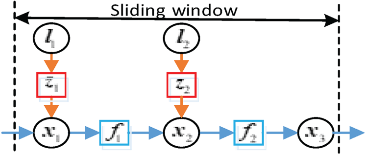
Figure 1. Express the VINS movement process using factor graphs

Therefore, the complete motion process of VINS can be represented by a factor graph as several dots and several edges connecting the dots. Each dot in the graph is the variable node to be optimised, and each edge connected to two variable nodes corresponds to a factor node, which is used to constrain the variable node. Through the construction of dots and edges, the error distribution structure of the visual–inertial system can be established intuitively, and the constraint relationship between variables can be displayed intuitively. For the factor graphs, its maximum posterior probability inference is equivalent to maximising the product of the potential energy of all factors (Dellaert and Kaess, Reference Dellaert and Kaess2017), which is also equivalent to minimising the solution of the nonlinear least squares problem. For the established graph, the numerical iterative method, like Gauss–Newton (GN) or Levenberg–Marquardt (LM), can be used to obtain the optimal solution of each factor node through a series of linear approximations.

Based on the factor graph optimisation, an improved VINS method named DSWFG is proposed. The following elaborates the DSWFG from three parts: the overall framework, the front-end processing method and the back-end processing method. Whenever there is an image frame input, the front-end part extracts the speeded up robust features (SURF) points on the image frame and uses the kanade-lucas-tomasi (KLT) tracking algorithm to track the feature points extracted from the previous image frame and takes the threshold constraint method to obtain the valid feature points of the current frame. At the same time, the front-end part uses the IMU pre-integration method to align the IMU with the image frame, then sends the processed IMU data and vision data to the back end. The back-end part limits the data operation scale with SWF and constructs the graph with the fixed number of states in the window using factor graphs. At the same time, the prior information of the sliding window is set dynamically to maintain the interframe constraint. The overall framework of DSWFG algorithm is shown in Figure 2. The following will be illustrated from the IMU pre-integration method in the front-end part, the construction of prior information of the sliding window in the back-end part and the optimisation of the states in the window.

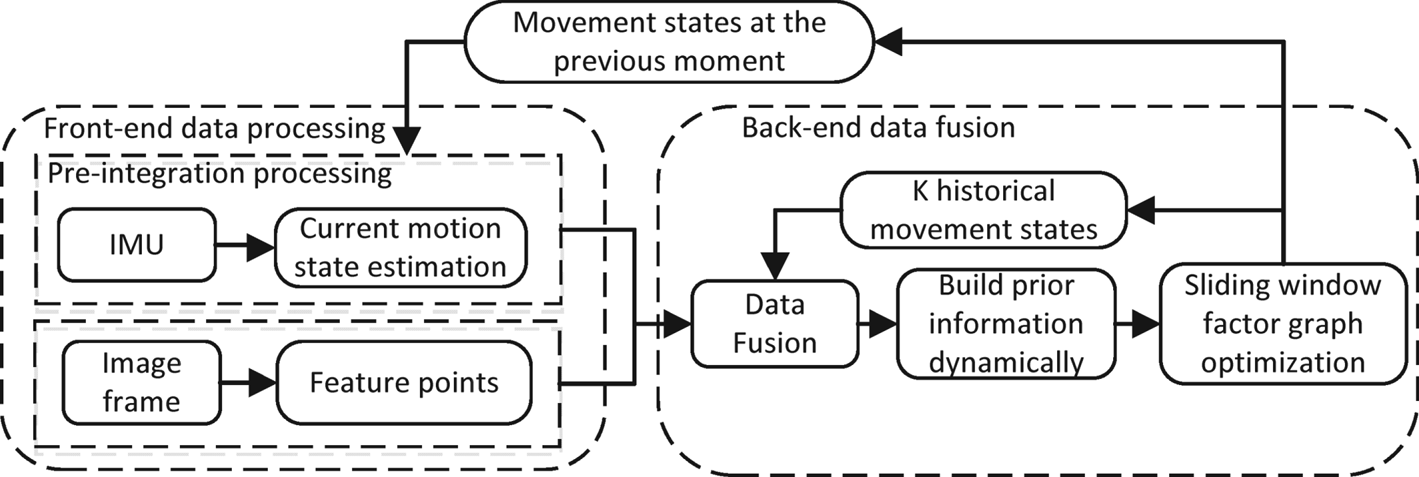
Figure 2. The overall framework of DSWFG algorithm

4.2. The IMU pre-integration method in the front-end part

Due to the high frequency of the IMU, there will be a large number of variable nodes added in the graph. Using the numerical iterative method to approximate the optimal solution of each factor node directly will result in less optimisation benefits for the high computational complexity. Therefore, a set of the IMU measurements between two adjacent image frames are integrated into a single relative motion constraint by the IMU pre-integration, and the processed IMU measurements are aligned with the image frames. Then, in the process of overall batch optimisation, the visual and IMU constraints can be considered at the same time, reducing the calculation burden and improving the optimisation effect. In addition, the IMU pre-integration method introduces the pre-integration term through an incremental expression, which can effectively avoid the recalculation of the IMU measurements during the optimisation process. The IMU pre-integration method in this section is based on the research of Forster (Forster et al., Reference Forster, Carlone, Dellaert and Scaramuzza2017), and the derivation process is as follows.

The motion relationship and the IMU noise model can be established as

(4.1)\begin{equation}\begin{cases} {{\tilde{{\boldsymbol w}}_{\rm B}}(t )= {{\boldsymbol w}_{\rm B}}(t )+ {{\boldsymbol b}_g}(t )+ {{\boldsymbol \eta }_g}(t )}\\ {{\tilde{{\boldsymbol a}}_{\rm B}}(t )= {\boldsymbol R}_{{\rm WB}}^{\rm T}({{{\boldsymbol a}_{\rm W}}(t )- {{\boldsymbol g}_{\rm W}}} )+ {{\boldsymbol b}_a}(t )+ {{\boldsymbol \eta }_a}(t )} \end{cases}\end{equation}

where ${\boldsymbol R}_{{\rm WB}}^{}$ represents rotation matrix from the carrier coordinate system ${\rm B}$ to world coordinate system ${\rm W}$. IMU angular velocity measurements ${{\boldsymbol w}_{\rm B}}$ are added bias ${{\boldsymbol b}_g}$ and noise ${{\boldsymbol \eta }_g}$. The measured values of IMU accelerometer $\tilde{{\boldsymbol a}_{\rm B}}$ are added bias ${{\boldsymbol b}_a}$ and noise ${{\boldsymbol \eta }_a}$. The differential motion model is established as

(4.2)\begin{equation}\begin{cases} {{\dot{\boldsymbol R}_{{\rm WB}}}} ={\boldsymbol R}_{{\rm WB}} {\boldsymbol w}_{\rm B}^\wedge \\ {{\dot{\boldsymbol v}_{\rm W}}} = {{\boldsymbol a}_{\rm W}}\\ {\dot{\boldsymbol p}_{\rm W}} = {{\boldsymbol v}_{\rm W}} \end{cases}\end{equation}

where the symbol $\wedge$ represents the transformation of the vector into an antisymmetric matrix. The discrete form of motion equation is obtained by Euler integral

(4.3)\begin{equation}\left\{ {\begin{array}{* {20}{l}} {{{\boldsymbol R}_{{\rm WB}}}({t + \Delta t} )={{\boldsymbol R}_{{\rm WB}}}(t ){\rm Exp}({{{\boldsymbol w}_{\rm B}}(t )\Delta t} )}\\ {{{\boldsymbol v}_{\rm W}}({t + \Delta t} )= {{\boldsymbol v}_{\rm W}}(t )+ {{\boldsymbol a}_{\rm W}}(t )\Delta t}\\ {{{\boldsymbol p}_{\rm W}}({t + \Delta t} )= {{\boldsymbol p}_{\rm W}}(t )+ {{\boldsymbol v}_{\rm W}}(t )\Delta t + \dfrac{1}{2}{{\boldsymbol a}_{\rm W}}(t )\Delta {t^2}} \end{array}} \right. \end{equation}

where $\Delta t$ = interval time between two adjacent IMU measurements. Combining the IMU noise model with Equation (4.3) gives

(4.4)\begin{equation}\begin{cases} {{{\boldsymbol R}_{{\rm WB}}}({t + \Delta t} )={{\boldsymbol R}_{{\rm WB}}}(t ){\rm Exp}\Big({\Big({{{\tilde{\boldsymbol w}}_{\rm B}}(t )- {{\boldsymbol b}_g}(t )- {{\boldsymbol \eta }_{gd}}(t )} \Big)\Delta t} \Big)}\\ {{{\boldsymbol v}_{\rm W}}({t + \Delta t} )= {{\boldsymbol v}_{\rm W}}(t )+ {{\boldsymbol g}_{\rm W}}\Delta t+{{\boldsymbol R}_{{\rm WB}}}\Big({{{\tilde{\boldsymbol a}}_{\rm B}}(t )- {{\boldsymbol b}_a}(t )- {{\boldsymbol \eta }_{ad}}(t )} \Big)\Delta t}\\ {{{\boldsymbol p}_{\rm W}}({t + \Delta t} )= {{\boldsymbol p}_{\rm W}}(t )+ {{\boldsymbol v}_{\rm W}}(t )\Delta t + \dfrac{1}{2}{{\boldsymbol g}_{\rm W}}\Delta {t^{2}}+\dfrac{1}{2}{{\boldsymbol R}_{{\rm WB}}}\Big({{{\tilde{\boldsymbol a}}_{\rm B}}(t )- {{\boldsymbol b}_a}(t )- {{\boldsymbol \eta }_{ad}}(t )} \Big)\Delta {t^{2}}} \end{cases}\end{equation}

where noise terms ${{\boldsymbol \eta }_{gd}}$ and ${{\boldsymbol \eta }_{ad}}$ are in discrete form, and the relationships between discrete noise and continuous noise are

(4.5)\begin{equation}\begin{cases} {{\rm Cov}({{{\boldsymbol \eta }_{gd}}(t )} ) = \dfrac{1}{{\Delta t}}{\rm Cov}({{{\boldsymbol \eta }_g}(t )} )}\\ {{\rm Cov}({{{\boldsymbol \eta }_{ad}}(t )} ) = \dfrac{1}{{\Delta t}}{\rm Cov}({{{\boldsymbol \eta }_a}(t )} )} \end{cases}\end{equation}

For symbol simplicity, the reference coordinate system in the formula is omitted. Assuming that the IMU measurements are aligned with the image frames, then the pose relationship between the adjacent image frames i and j can be obtained as

(4.6)\begin{equation}\begin{cases} {{{\boldsymbol R}_j}={{\boldsymbol R}_j}\displaystyle\prod_{k = i}^{j - 1} {\rm Exp}\Big({\Big({{{\tilde{\boldsymbol w} }_k}{- }{\boldsymbol b}_k^g{- }{\boldsymbol \eta }_k^{gd}} \Big)\Delta t} \Big)}\\ {{{\boldsymbol v}_j} = {{\boldsymbol v}_i} + {\boldsymbol g}\Delta {t_{ij}}+\displaystyle\sum\limits_{k = i}^{j - 1} {{{\boldsymbol R}_k}\Big({{{\tilde{\boldsymbol a} }_k} - {\boldsymbol b}_k^a - {\boldsymbol \eta }_k^{ad}} \Big)\Delta t} }\\ {{{\boldsymbol p}_j} = {{\boldsymbol p}_i} + \displaystyle\sum\limits_{k = i}^{j - 1} {\left[ {{{\boldsymbol v}_k}\Delta t + \dfrac{1}{2}{\boldsymbol g}\Delta {t^{2}} + +\dfrac{1}{2}{\boldsymbol R}_k^{}\Big({{{\tilde{\boldsymbol a} }_k} - {\boldsymbol b}_k^a - {\boldsymbol \eta }_k^{ad}} \Big)\Delta {t^{2}}} \right]} } \end{cases} \end{equation}

In order to avoid solving ${\boldsymbol R}_i^{}$, ${{\boldsymbol v}_i}$, ${{\boldsymbol p}_i}$ again, introduce the pre-integration term through incremental expression

(4.7)\begin{equation}\begin{cases} {\Delta {{\boldsymbol R}_{ij}}={\boldsymbol R}_i^{\rm T}{{\boldsymbol R}_i} = \displaystyle\prod_{k = i}^{j - 1} {\rm Exp}\Big({\Big({{{\tilde{\boldsymbol w}}_k}{- }{\boldsymbol b}_k^g{- }{\boldsymbol \eta }_k^{gd}} \Big)\Delta t} \Big)}\\ {\Delta {{\boldsymbol v}_{ij}} = {\boldsymbol R}_i^{\rm T}({{{\boldsymbol v}_j} - {{\boldsymbol v}_i} - {\boldsymbol g}\Delta {t_{ij}}} )= \displaystyle\sum_{k = i}^{j - 1} {{{\boldsymbol R}_{ik}}\Big({{{\tilde{\boldsymbol a} }_k}{- }{\boldsymbol b}_k^a{- }{\boldsymbol \eta }_k^{ad}} \Big)\Delta t} }\\ {\Delta {{\boldsymbol p}_{ij}} = {\boldsymbol R}_i^{\rm T}\left( {{{\boldsymbol p}_j} - {{\boldsymbol p}_i} - {{\boldsymbol v}_i}\Delta {t_{ij}} + \dfrac{1}{2}{\boldsymbol g}\Delta t_{ij}^2} \right) = \displaystyle\sum_{k = i}^{j - 1} {\left[ {{{\boldsymbol v}_{ik}}\Delta t+\dfrac{1}{2}{{\boldsymbol R}_{ik}}\Big({{{\tilde{\boldsymbol a}}_k}{- }{\boldsymbol b}_k^a{- }{\boldsymbol \eta }_k^{ad}} \Big)\Delta {t^{2}}} \right]} } \end{cases}\end{equation}

Therefore, the IMU constraints between image frames can be obtained by the IMU measurements between two adjacent image frames.

4.3. The construction of prior information in the back-end part

Based on the front-end IMU pre-integration method, the IMU measurements are aligned with the image frames, and the processed data collected from IMU and visual sensor are sent to the back end. The back-end part limits the amount of data with the sliding window and constructs the graph with the fixed number of states in the window using factor graph optimisation method. At the same time, the prior information of the current sliding window is set dynamically to maintain the interframe constraint. The processing flow of SWF is shown in Figure 3.

Figure 3. The processing flow of SWF

Once the image frame has been acquired, the front-end data processing module outputs observation information and motion state of the current image frame and integrates it into the sliding window as the current frame information. In order to maintain a fixed number of K image frames within a window, the historical image frames in the window must be processed. Then, the oldest image frame in the window is removed. Therefore, once a new image frame has been acquired, the current frame information is added to the rear end of the window, and the oldest image frame at the front of the window is removed at the same time.

If the oldest image frame in the window is directly removed and only the internal states in the window are optimised, then the inter-frame constraint will be lost. That is, there is an IMU constraint between the image frame removed and the adjacent image frame in the window. Only performing optimisation operations on the internal states in the window will easily cause the optimised states not meet the IMU constraint, which affects the overall estimate precision.

Therefore, the oldest image frame cannot be directly removed. The constraint between the oldest and the adjacent image frame in the window needs to be considered. Once new image frame has been acquired, the image frame to be removed is determined and the motion state corresponding to the image frame removed is selected as the priori information. Since the state corresponding to the removed image frame has undergone multiple optimisation estimates, it can be considered that the state corresponding to the removed image frame can be fixed without being optimised again. Select it as the prior information of current sliding window and form the IMU constraint with the state corresponding to the adjacent image frame. In the subsequent optimisation, it can be used to constrain the states to be optimised, remove the error measurement information and fix the problem of states mutation caused by the input of wrong states, so that ensure the accuracy of the estimates.

The triangulation method (Richard and Zisserman, Reference Richard and Zisserman2000) is used to estimate the spatial positions of M landmarks observed by the K image frames in the window to form interframe observation constraints. Combined with the estimations of motion states, interframe motion constraints and observation constraints are established. The corresponding logical relationship is constructed using factor graphs, and the numerical iterative method is used to approximate the optimal solutions of K motion states in the window. Then, the motion state corresponding to the oldest image frame of current window is selected and used as the output of current sliding window.

4.4. The optimisation of the states in the window

Based on the data processing of the current sliding window, K motion states, M spatial positions of landmarks and the prior information of current sliding window are obtained. The graph is constructed with the data obtained. Then the optimisation of graph is equivalent to the least squares problem inside the window. For the established graph, use the LM method to obtain the optimal solution of each factor node through a series of linear approximations. The processing flow of factor graph optimisation is shown in Figure 4.

Figure 4. The processing flow of factor graph optimisation

The state ${\boldsymbol x}$ is constituted with K motion states ${{\boldsymbol x}_n}$ in current sliding window, M landmarks ${{\boldsymbol l}_n}$ observed by the K motion states, as well as the priori information ${{\boldsymbol x}_{{\rm pri}}}$, which can be written as

(4.8)\begin{equation} {\boldsymbol x} = \{{{{\boldsymbol x}_{{\rm pri}}},{{\boldsymbol x}_{\rm 1}},\ldots ,{{\boldsymbol x}_K},{{\boldsymbol l}_1},\ldots ,{{\boldsymbol l}_M}} \} \end{equation}

where the state ${{\boldsymbol x}_n}$ includes the position and rotation of the carrier, ${{\boldsymbol l}_m}=\left[ {\begin{array}{* {20}{c}} {{x_m}}&{{y_m}}&{{z_m}} \end{array}} \right]$ and ${}^{\rm c}{{\boldsymbol l}_m}=\left[ {\begin{array}{* {20}{c}} {{}^{\rm c}{x_m}}&{{}^{\rm c}{y_m}}&{{}^{\rm c}{z_m}} \end{array}} \right]$ refer to the spatial positions of the m ^th landmark in the world coordinate and camera coordinate system, respectively. Showing non-zero blocks only, the sparse matrix ${\boldsymbol H}$ is constructed as

(4.9)\begin{equation}{\boldsymbol H} = \left[ {\begin{array}{* {20}{c}} { - {{\boldsymbol H}_{{\boldsymbol x},1}}}&{\rm 1}&{}&{}&{}\\ {}&{ - {{\boldsymbol G}_{{\boldsymbol x},1}}}&{}&{}&{ - {{\boldsymbol G}_{{\boldsymbol l},1}}}\\ {}&{}&{\ldots }&{\ldots }&{\ldots }\\ {}&{}&{ - {{\boldsymbol H}_{{\boldsymbol x},K}}}&{\rm 1}&{}\\ {}&{}&{}&{ - {{\boldsymbol G}_{{\boldsymbol x},K}}}&{ - {{\boldsymbol G}_{{\boldsymbol l},K}}} \end{array}} \right]\end{equation}

where ${{\boldsymbol H}_{{\boldsymbol x},n}}$ is a ${\rm 6} \times {\rm 6}$ Jacobian matrix

(4.10)\begin{equation}{{\boldsymbol H}_{{\boldsymbol x},n}} = \left[ {\begin{matrix} {\dfrac{{\partial {\boldsymbol e}_{{\rm IMU}}^n}}{{\partial {{\boldsymbol p}_n}}}}&{\dfrac{{\partial {\boldsymbol e}_{{\rm IMU}}^n}}{{\partial {{\boldsymbol R}_n}}}} \end{matrix}} \right] = \left[ {\begin{matrix} {\dfrac{{\partial {}^{\rm P}{\boldsymbol e}_{{\rm IMU}}^n}}{{\partial {{\boldsymbol p}_n}}}}&{\dfrac{{\partial {}^{\rm P}{\boldsymbol e}_{{\rm IMU}}^n}}{{\partial {{\boldsymbol R}_n}}}}\\ {\dfrac{{\partial {}^{\rm R}{\boldsymbol e}_{{\rm IMU}}^n}}{{\partial {{\boldsymbol p}_n}}}}&{\dfrac{{\partial {}^{\rm R}{\boldsymbol e}_{{\rm IMU}}^n}}{{\partial {{\boldsymbol R}_n}}}} \end{matrix}} \right] \end{equation}

where IMU error ${\boldsymbol e}_{{\rm IMU}}^n$ = difference between the pre-integration term and the state solved by the IMU measurements at epoch n, including position error ${}^{\rm P}{\boldsymbol e}_{{\rm IMU}}^n$ and rotation error ${}^{\rm R}{\boldsymbol e}_{{\rm IMU}}^n$; ${{\boldsymbol R}_n}$ = rotation matrix at epoch n; ${{\boldsymbol p}_n}$ = the position at epoch n; and ${{\boldsymbol G}_{{\boldsymbol x},n}}$ = a ${2}m \times {\rm 6}$ matrix, where m is determined by the number of landmarks observed in the current observation frame, that is

(4.11)\begin{equation}{{\boldsymbol G}_{{\boldsymbol x},n}}={[{{\boldsymbol G}_{{\boldsymbol x},n}^{\rm 1},\ldots ,{\boldsymbol G}_{{\boldsymbol x},n}^m} ]^{\rm T}}\end{equation}

where ${\boldsymbol G}_{{\boldsymbol x},n}^m$ is a ${2} \times {\rm 6}$ Jacobian matrix

(4.12)\begin{equation}{\boldsymbol G}_{{\boldsymbol x},n}^m=\left[ {\begin{array}{* {20}{c}} {\dfrac{{\partial {\boldsymbol e}_{{\rm VIS}}^m}}{{\partial {{\boldsymbol p}_n}}}}&{\dfrac{{\partial {\boldsymbol e}_{{\rm VIS}}^m}}{{\partial {{\boldsymbol R}_n}}}} \end{array}} \right]=\left[ {\begin{array}{* {20}{c}} {\dfrac{{\partial {\boldsymbol e}_{{\rm VIS}}^m}}{{\partial {}^{\rm c}{{\boldsymbol l}_m}}}\dfrac{{\partial {}^{\rm c}{{\boldsymbol l}_m}}}{{\partial {{\boldsymbol p}_n}}}}&{\dfrac{{\partial {\boldsymbol e}_{{\rm VIS}}^m}}{{\partial {}^{\rm c}{{\boldsymbol l}_m}}}\dfrac{{\partial {}^{\rm c}{{\boldsymbol l}_m}}}{{\partial {{\boldsymbol R}_n}}}} \end{array}} \right]\end{equation}

where ${\boldsymbol e}_{{\rm VIS}}^m=\left[ {\begin{array}{* {20}{c}} {{}^{\rm u}{\boldsymbol e}_{{\rm VIS}}^m}&{{}^{\rm v}{\boldsymbol e}_{{\rm VIS}}^m} \end{array}} \right]$ = observation error of the m ^th landmark projected in the pixel coordinate system at epoch n.

(4.13)\begin{equation}{\boldsymbol g} = \frac{{\partial {\boldsymbol e}_{{\rm VIS}}^m}}{{\partial {}^{\rm c}{{\boldsymbol l}_m}}}=\left[ {\begin{matrix} {\dfrac{{\partial {}^{\rm u}{\boldsymbol e}_{{\rm VIS}}^m}}{{\partial {}^{\rm c}{x_m}}}}&{\dfrac{{\partial {}^{\rm u}{\boldsymbol e}_{{\rm VIS}}^m}}{{\partial {}^{\rm c}{y_m}}}}&{\dfrac{{\partial {}^{\rm u}{\boldsymbol e}_{{\rm VIS}}^m}}{{\partial {}^{\rm c}{z_m}}}}\\ {\dfrac{{\partial {}^{\rm v}{\boldsymbol e}_{{\rm VIS}}^m}}{{\partial {}^{\rm c}{x_m}}}}&{\dfrac{{\partial {}^{\rm v}{\boldsymbol e}_{{\rm VIS}}^m}}{{\partial {}^{\rm c}{y_m}}}}&{\dfrac{{\partial {}^{\rm v}{\boldsymbol e}_{{\rm VIS}}^m}}{{\partial {}^{\rm c}{z_m}}}} \end{matrix}} \right] \end{equation}

${{\boldsymbol G}_{{\boldsymbol l},n}}$ is a ${2}m \times {\rm 6}m$ matrix, where m is determined by the number of landmarks observed in the current observation frame. ${{\boldsymbol G}_{{\boldsymbol l},n}}$ is expressed as

(4.14)\begin{equation}{{\boldsymbol G}_{{\boldsymbol l},n}}=\left[ {\begin{array}{* {20}{c}} {{\boldsymbol G}_{{\boldsymbol l},n}^{\rm 1}}&{}&{}\\ {}&{{\boldsymbol G}_{{\boldsymbol l},n}^2}&{}\\ {}&{\ldots }&{}\\ {}&{}&{{\boldsymbol G}_{{\boldsymbol l},n}^m} \end{array}} \right] \end{equation}

where ${\boldsymbol G}_{{\boldsymbol l},n}^m$ is a ${2} \times {\rm 3}$ Jacobian matrix

(4.15)\begin{equation}{\boldsymbol G}_{{\boldsymbol l},n}^m=\frac{{\partial {\boldsymbol e}_{{\rm VIS}}^m}}{{\partial {{\boldsymbol l}_m}}}=\left[ {\begin{array}{* {20}{c}} {\dfrac{{\partial {\boldsymbol e}_{{\rm VIS}}^m}}{{\partial {}^{\rm c}{{\boldsymbol l}_m}}}\dfrac{{\partial {}^{\rm c}{{\boldsymbol l}_m}}}{{\partial {{\boldsymbol l}_m}}}}&{\dfrac{{\partial {\boldsymbol e}_{{\rm VIS}}^m}}{{\partial {}^{\rm c}{{\boldsymbol l}_m}}}\dfrac{{\partial {}^{\rm c}{{\boldsymbol l}_m}}}{{\partial {{\boldsymbol l}_m}}}} \end{array}} \right]\end{equation}

The K IMU observation errors ${\boldsymbol e}_{{\rm IMU}}^n$ and M landmarks observation errors ${\boldsymbol e}_{{\rm VIS}}^m$ are stacked to form the internal error vector ${\boldsymbol e}$ in current sliding window. ${\boldsymbol \varSigma }$ = total covariance, the structure is

(4.16)\begin{equation}{\boldsymbol e} = \left[ {\begin{matrix} {{\boldsymbol e}_{{\rm IMU}}^1}\\ {\ldots }\\ {{\boldsymbol e}_{{\rm IMU}}^K}\\ {{\boldsymbol e}_{{\rm VIS}}^1}\\ {\ldots }\\ {{\boldsymbol e}_{{\rm VIS}}^M} \end{matrix}} \right],{{\boldsymbol \varSigma }^{ - 1}}=\left[ {\begin{matrix} {{\boldsymbol \varSigma }_0^{ - 1}}&{}&{}&{}&{}&{}\\ {}&{\ldots }&{}&{}&{}&{}\\ {}&{}&{{\boldsymbol \varSigma }_K^{ - 1}}&{}&{}&{}\\ {}&{}&{}&{{\boldsymbol \varSigma }_{K+1}^{ - 1}}&{}&{}\\ {}&{}&{}&{}&{\ldots }&{}\\ {}&{}&{}&{}&{}&{{\boldsymbol \varSigma }_{K+M}^{ - 1}} \end{matrix}} \right]\end{equation}

Form linear equations corresponding to all states in current sliding window for linear optimisation

(4.17)\begin{equation}({{{\boldsymbol H}^{\rm T}}{{\boldsymbol \varSigma }^{{- }1}}{\boldsymbol H}} )\delta {\boldsymbol x}= - {\boldsymbol H}{{\boldsymbol \varSigma }^{ - 1}}{\boldsymbol e}\end{equation}

According to the construction of factor graphs, motion state estimations in the current sliding window are determined jointly by the motion states, landmark positions and prior information. Since the state related to the prior information is fixed, the algorithm does not need to solve the increment related to the fixed value during optimisation process. Then the dimension of matrix ${\boldsymbol H}$ can be reduced and the influence of prior information can be kept, so that the computational complexity is reduced, and the incremental solution is not affected.

The overall state increment is obtained by solving the linear equation, and the node state is corrected multiple times using the overall state increment. Combined with the prior information of the current sliding window, the optimal estimations of states in the window can be obtained and fed back to the window for the next optimisation operation.

5.1. Experimental environment and design

To validate the new method, the comparative experiments are designed between the optimal filtering methods and factor graph optimisation method. Based on the EKF, InEKF and the proposed DSWFG method, the karlsruhe institute of technology and toyota institute of technology (KITTI) dataset is selected as the experimental environment. The KITTI dataset is a combination of image frames, trajectory data and IMU data collected by the autonomous driving platform driving in different complex scenarios, such as cities, villages and highways (Geiger et al., Reference Geiger, Lenz, Stiller and Urtasun2012). The experiments mainly use the grayscale images provided by the dataset fragments, the IMU measurements provided by the OXTS RT 3003 positioning system, and the real position and attitude data to test the effect of the algorithm. The synchronised IMU output rate and image output rate are both 10Hz.

In this paper, the motion trajectory estimation, pose error statistics, and single-cycle time consuming are analysed to verify the proposed DSWFG algorithms. The setting of the sliding window range and the maximum number of optimisation iterations greatly affect the accuracy and real-time performance of the DSWFG algorithm. In order to ensure that the experiment results in different scenes are not affected by the change of parameters, the parameters of the sliding window range and the maximum number of iterations are fixed. Then, the range is set to 10, and the maximum number is set to 6. And the simulation is processed in the Matlab R2016 on a PC with Intel Core i5-9400 CPU at 2⋅90 GHz, 8-GB RAM equipped with Windows 10. The main noise parameters and variances are shown in Table 1.

Table 1. Experimental parameters

5.2. Multi-scenario comparison experiments

5.2.1. The residential area driving scene

The dataset sequence named 2011_09_26_drive_0036 is used. In order to establish a table for further quantitative analysis, the dataset segment name is abbreviated as 26–36. The dataset contains 803 image frames and a total of 715 meters of residential area driving. This scene contains the driving process of two right-angle turns. Figure 5 intuitively describes the results of the EKF, InEKF and DSWFG algorithms on this dataset segment. The lines in Figure 5(a) represent the real motion trajectory Vs. the estimated trajectory of each algorithm. In Figures 5(b) and 5(c), each algorithm is evaluated by three-directional position errors and attitude angle errors.

Figure 5. Results of residential area scene using the 26–36 dataset. (a) The real trajectory vs. calculated trajectories. (b) The attitude error. (c) The position error

Before the second right-angle bend, it can be seen that the motion trajectories estimated by the three algorithms are basically consistent with the real trajectory, and the main error lies in the turning of the real trajectory. At the second right-angle turn, which is at frame 338, the driving platform encounters and follows a truck. Because the distance between the driving platform and the truck is relatively close, a huge moving object affects the constraints of landmarks. Then, it makes the position drift using the EKF and InEKF. It can also be seen that the InEKF and EKF have a certain degree of divergence in attitude and position estimation error from the frame 338. In comparison, the InEKF is superior to the EKF. And from an overall perspective, the DSWFG algorithm achieves optimal stability and superior estimation accuracy in this scenario.

5.2.2. The city driving scene

The dataset sequence named 2011_09_30_drive_0018 is used, and the dataset segment name is abbreviated as 30–18. The first 1200 image frames and a total of 872 meters of city driving are used for simulation. This scene contains the driving process of four right-angle turns. During this traversal, Figure 6 intuitively describes the results of the EKF, InEKF and DSWFG algorithms on this dataset segment.

Figure 6. Results of city driving scene using the 30–18 dataset. (a) The real trajectory vs. calculated trajectories. (b) The attitude error. (c) The position error

Before the third right-angle bend, it can be seen that the motion trajectories estimated by the three algorithms are basically consistent with the real trajectory. At the 887th frame and the 1134th frame around the fourth right-angle turn, there are moving objects, which last about 30 frames and 20 frames, respectively. The common effect of moving objects and right-angle bending causes the divergence of the trajectory estimated by the InEKF and leads to worse estimation accuracy. Due to the accumulation of errors, the estimation accuracy of EKF is much lower than the DSWFG algorithm. At the same time, it can also be seen from Figures 6(b) and 6(c) that the position estimation error of the InEKF starts to diverge from the 1134th frame, while the EKF algorithm and the DSWFG algorithm can still maintain good stability. The overall comparison shows that the DSWFG algorithm achieves the best stability and superior estimation accuracy in this scenario.

5.2.3. The highway driving scene

The dataset sequence named 2011_10_03_drive_0042 is used, and the dataset segment name is abbreviated as 03–42. The 1170 image frames and a total of 2566 meters of highway driving area are used. This scene records the driving process of getting on and off the highway, which includes a starting curve and a final 360-degree circular curve. In this traversal process, Figure 7 describes the results of the EKF, InEKF and DSWFG algorithms. Given that the number of vehicles on the highway are few and other vehicles are relatively fast in this dataset fragment, the impact of moving objects is relatively small.

Figure 7. Results of highway driving scene using the 03–42 dataset. (a) The real trajectory vs. calculated trajectories. (b) The attitude error. (c) The position error

It can be seen that the movement trajectories solved by three verified algorithms are basically consistent with the real trajectory in Figure 7(a). The motion trajectories solved by the DSWFG algorithm and EKF algorithm almost match the real trajectory, especially in the middle of the real trajectory. Due to the influence of dynamic objects at the beginning, the trajectory obtained by the InEKF is deviated, which in turn affects the accuracy of the subsequent trajectory.

5.2.4. Statistical analysis

In addition to the typical three sets of experimental results above, more experiments were carried out for quantitative analysis. Table 2 shows the error statistical results of seven driving scenes, including rural roads, circular driving, complex loops and highways. The bold part indicates that the result is relatively optimal. Based on the comparison results of the three algorithms, it can be seen that the DSWFG algorithm can still maintain a good solution result in various sports scenarios. In order to compare the results of the three algorithms accurately, the root-mean-square error (RMSE) in three directions and the computing time are taken as the evaluation index. The following conclusions can be drawn from Table 2:

1. (a) From the results of sequences 26–36, 30–18, 30–33, 30–34 and 03–42, it can be seen that the DSWFG algorithm has better accuracy than the InEKF and EKF algorithms in terms of position and attitude errors.

2. (b) From the results of sequences 26–19 and 30–20, it can be seen the EKF are slightly better than the DSWFG algorithm in some ways. However, considering the overall estimation accuracy of the position and attitude, the DSWFG algorithm has better accuracy than do the InEKF and EKF algorithms.

3. (c) Analysing the time consuming of a single cycle, an overall comparison shows that the InEKF algorithm is the fastest, while the DSWFG algorithm is relatively slow.

4. (d) The real-time performance of the InEKF is superior to the other two algorithms, and its accuracy is generally better than the traditional EKF method under the ideal conditions during the background environment is stationary. However, with the influence of moving objects, the stability of the InEKF is poor, and its motion trajectory is easy to diverge. The real-time performance of the DSWFG is relatively poor, but the comparison results in various motion scenes show that it can maintain the superior accuracy and optimal stability.

Table 2. Results of EKF, InEKF and DSWFG