


1. INTRODUCTION
Spherical trigonometry formulae are widely applied to solve the various spherical geometry problems in different fields such as navigation, aviation, geodesy and astronomy. The main spherical trigonometry formulae are the formulae of a right spherical triangle, the formulae of a quadrantal spherical triangle, the law of sines, the law of cosines for the sides, the law of cosines for the angles, the half-angle formulae, the half-side formulae, the four-part formulae, the five-part formulae, Delambre's analogies, Napier's analogies, Cagnoli's formulae, etc. Many textbooks have presented different approaches to derive these formulae, for example: Clough-Smith (Reference Clough-Smith1978), Todhunter (1886) and Smart (Reference Smart1977) provided a geometric method for gnomonic projection to derive the law of cosines for the sides. Green (Reference Green1985) introduced a vector method to derive the law of cosines for the sides. Murray (Reference Murray1908) and Wentworth and Smith (Reference Wentworth and Smith1915) used the formulae of a right spherical triangle to derive the law of cosines for the sides. We can acquire these formulae and related knowledge from many textbooks or on websites such as MathWorld (1999) and Wikipedia (2001).
In fact, these spherical trigonometry formulae are all used to express the relationships between the six variables of a single spherical triangle. The six variables include the three sides (a, b, and c) and three angles (α, β, and γ) as shown in Figure 1. For example, the variable relationships of the law of cosines for the sides are the opposite relations between three sides and one angle. The variable relationships of the four-part formulae are the adjacent relations between two sides and two angles. The advantage of these formulae is that they are convenient to apply. If the given variables match the precondition of a particular formula, the unknown variables can be directly obtained by using that formula. For instance, when two sides and their included angle are given, the third side can be directly obtained by using the law of cosines for the sides.
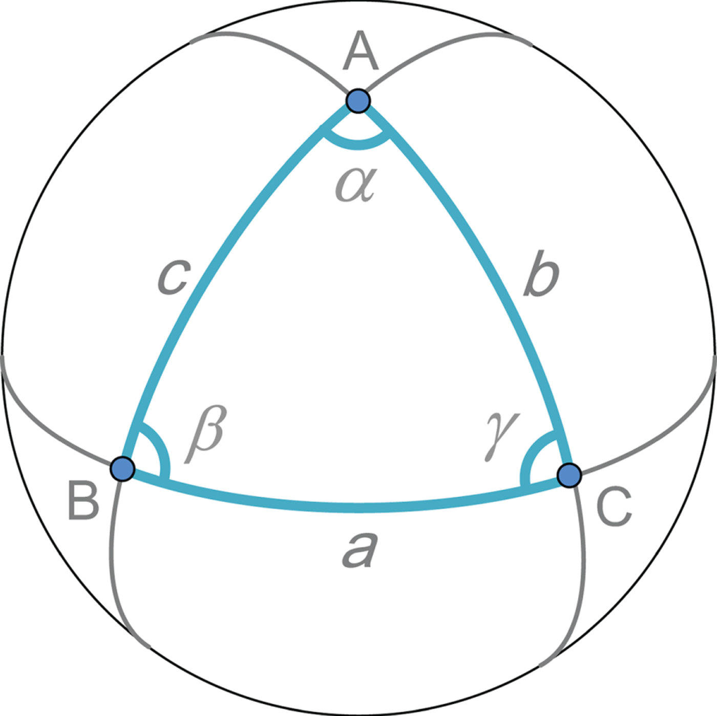
Figure 1. Illustration of the single spherical triangle.
However, the current spherical trigonometry formulae only express the relationships between the sides and angles of a single spherical triangle. Many problems may involve different types of spherical shapes such as spherical quadrilaterals and spherical polygons, which cannot be directly solved by adopting single spherical triangle formulae. Therefore, we propose two types of formulae for combined spherical triangles, which are the formulae of the divided spherical triangle and the formulae of the spherical quadrilateral.
2. FORMULAE OF THE DIVIDED SPHERICAL TRIANGLE
In the case of the divided spherical triangle, the spherical triangle may be divided from one angle or one side as shown in Figure 2. In the given divided angle condition, the spherical triangle ( ${\mathop{\Delta} \limits^{\frown}}\hbox{ABC}$) is divided from the angle α into two spherical triangles (
 ${\mathop{\Delta} \limits^{\frown}}\hbox{ABX}$ and
  ${\mathop{\Delta} \limits^{\frown}}\hbox{AXC}$). When the two sides (c and b) and the divided angles (α, α 1 and α 2) are given, the other angles (β and γ) can be obtained by using the four-part formulae, and the side a can be obtained by using the law of cosines for the sides. However, none of formulae of the single spherical triangle can directly find the side x (which we called the common side). Similarly, in the given divided side condition, the spherical triangle (
 ${\mathop{\Delta} \limits^{\frown}}\hbox{ABC}$) is divided from the side a into two spherical triangles (
 ${\mathop{\Delta} \limits^{\frown}}\hbox{ABX}$ and
  ${\mathop{\Delta} \limits^{\frown}}\hbox{AXC}$). When the two sides (c and b) and the divided sides (a, a 1 and a 2) are given, none of formulae of the single spherical triangle can directly find the common side (x). Therefore, we propose the formulae of the divided spherical triangle as follows.
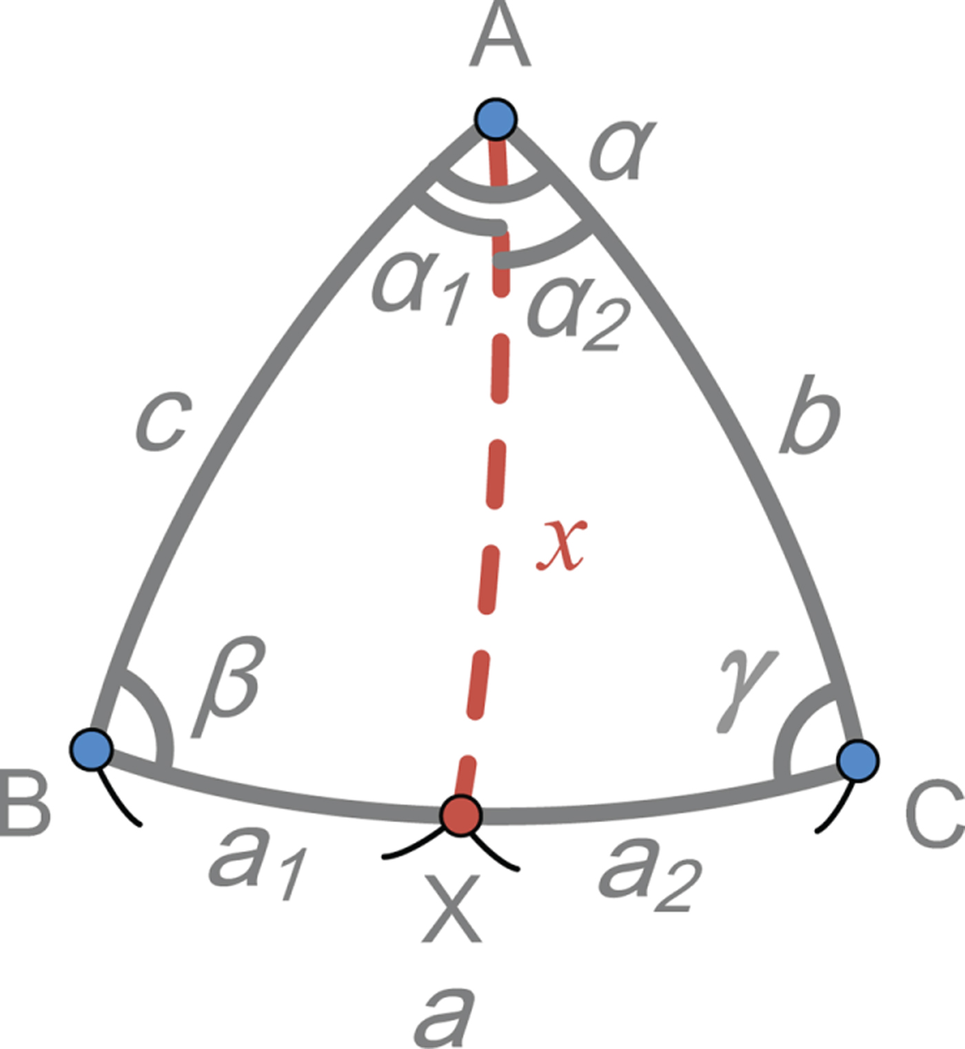
Figure 2. Illustration of the divided spherical triangle.
First, list the four-part formulae of the two spherical triangles ( ${\mathop{\Delta} \limits^{\frown}}\hbox{ABC}$ and
  ${\mathop{\Delta} \limits^{\frown}}\hbox{ABX}$) in Figure 2:
 $$\tan\beta=\displaystyle{{\sin\alpha}\over{\sin c\cot b-\cos c\cos\alpha}} $$
 $$\tan\beta=\displaystyle{{\sin\alpha_{1}}\over{\sin c\cot x-\cos c\cos\alpha_{1}}} $$
Substitute Equation (1) into Equation (2), and rearrange the formula:
 $$\tan x=\displaystyle{{\sin\alpha}\over{\sin\alpha_{1}\cot b+\sin\alpha_{2}\cot c}} $$
 Then, list the law of cosines for the sides of the two spherical triangles ( ${\mathop{\Delta} \limits^{\frown}}\hbox{ABC}$ and
  ${\mathop{\Delta} \limits^{\frown}}\hbox{ABX}$) in Figure 2:
 $$\cos\beta=\displaystyle{{\cos b-\cos c\cos a}\over{\sin c \sin a}} $$
 $$\cos\beta=\displaystyle{{\cos x-\cos c\cos a_{1}}\over{\sin c\sin a_{1}}} $$
Substitute Equation (4) into Equation (5), and rearrange the formula:
 $$\cos x=\displaystyle{{\sin a_{1}\cos b+\sin a_{2}\cos c}\over{\sin a}} $$
As a result, Equation (3) is the formula of the common side (x) in the given divided angle condition, and Equation (6) is the formula of the common side (x) in the given divided side condition.
3. FORMULAE OF THE SPHERICAL QUADRILATERAL
In the case of the spherical quadrilateral, its shape may be concave or convex. For example, in the concave shape condition as shown in Figure 3(a), the two spherical triangles ( ${\mathop{\Delta} \limits^{\frown}}\hbox{ABC}$ and
  ${\mathop{\Delta} \limits^{\frown}}\hbox{ACD}$), which have the common side b (that is, side d), combine to one spherical quadrilateral (
 ${\mathop{\Delta} \limits^{\frown}}\hbox{ABCD}$). When the four sides (c 1, a 1, c 2 and a 2) and the combined angle (α 3) are given, the side a 3 can be obtained by using the law of cosines for the sides. However, none of formulae of the single spherical triangle can directly find the angle γ 3 and the angle β 1. Similarly, in the convex shape condition as shown in Figure 3(b), none of formulae of the single spherical triangle can directly find the angle γ 3 and the angle β 1, either. Thus, we propose the formulae which can directly obtain the auxiliary angle (γ 3) and the outer angles (β 1) as follows.

Figure 3. Illustration of the spherical quadrilateral.
First, list the law of cosines for the sides of the two spherical triangles ( ${\mathop{\Delta} \limits^{\frown}}\hbox{ABD}$ and
  ${\mathop{\Delta} \limits^{\frown}}\hbox{CBD}$) in Figure 3(a):
 $$\cos a_{3}=\cos c_{1}\cos c_{2}+\sin c_{1}\sin c_{2}\cos\alpha_{3} $$
 $$\cos a_{3}=\cos a_{1}\cos a_{2}+\sin a_{1}\sin a_{2}\cos\gamma_{3} $$
Substitute Equation (7) into Equation (8), and rearrange the formula to derive the formula of the auxiliary angle (γ 3):
 $$\cos\gamma_{3}=\displaystyle{{\cos c_{1}\cos c_{2}-\cos a_{1}\cos a_{2}+\sin c_{1}\sin c_{2}\cos\alpha_{3}}\over{\sin a_{1}\sin a_{2}}} $$
 Then, list the four-part formulae of the two spherical triangles ( ${\mathop{\Delta} \limits^{\frown}}\hbox{ABD}$ and
  ${\mathop{\Delta} \limits^{\frown}}\hbox{CBD}$) in Figure 3(a):
 $$\tan\beta_{3}=\displaystyle{{\sin\alpha_{3}}\over{\sin c_{1}\cot c_{2}-\cos c_{1}\cos\alpha_{3}}} $$
 $$\tan\beta_{2}=\displaystyle{{\sin\gamma_{3}}\over{\sin a_{1}\cot a_{2}-\cos a_{1}\cos\gamma_{3}}} $$
Use Equation (10), (11), and the addition formula of trigonometric functions to derive the formula of the outer angle (β 1), where β 1 = β 3 − β 2:
 $$\tan\beta_{1}=\displaystyle{{\sin\alpha_{3}\lpar \sin a_{1}\cot a_{2}-\cos a_{1}\cos\gamma_{3}\rpar -\sin\gamma_{3}\lpar \sin c_{1}\cot c_{2}-\cos c_{1}\cos\alpha_{3}\rpar }\over{\lpar \sin c_{1}\cot c_{2}-\cos c_{1}\cos\alpha_{3}\rpar \lpar \sin a_{1}\cot a_{2}-\cos a_{1}\cos\gamma_{3}\rpar +\sin\alpha_{3}\sin\gamma_{3}}} $$
Note that in the convex shape condition as shown in Figure 3(b), the formula of the auxiliary angle (γ 3) is the same formula as Equation (9), but the formula of the outer angle (β 1), where β 1 = β 3 + β 2, should be substituted as follows:
 $$\tan\beta_{1}=\displaystyle{{\sin\alpha_{3}\lpar \sin a_{1}\cot a_{2}-\cos a_{1}\cos\gamma_{3}\rpar +\sin\gamma_{3}\lpar \sin c_{1}\cot c_{2}-\cos c_{1}\cos\alpha_{3}\rpar }\over{\lpar \sin c_{1}\cot c_{2}-\cos c_{1}\cos\alpha_{3}\rpar \lpar \sin a_{1}\cot a_{2}-\cos a_{1}\cos\gamma_{3}\rpar -\sin\alpha_{3}\sin\gamma_{3}}} $$
Hence, Equations (9) and (12) are the formulae of the auxiliary angle (γ 3) and the outer angle (β 1) in the concave shape condition, and Equations (9) and (13) are the formulae of the auxiliary angle (γ 3) and the outer angle (β 1) in the convex shape condition.
Since the spherical quadrilateral can also be seen as the divided spherical triangle when the auxiliary angle (γ 3) is 180°, the formulae of the divided spherical triangle can be derived from the formulae of the spherical quadrilateral as follows:
First, substitute 180° into the auxiliary angle (γ 3) in Equation (12) and Equation (13), and rearrange the formula:
 $$\tan\beta_{1}=\displaystyle{{\sin\alpha_3}\over{\lpar \sin c_{1}\cot c_{2}-\cos c_{1}\cos\alpha_{3}\rpar }} $$
 Then, list the four-part formulae of the spherical triangle ( ${\mathop{\Delta} \limits^{\frown}}\hbox{ABC}$) in Figure 3(a) and Figure 3(b):
 $$\tan\beta_{1}=\displaystyle{{\sin \alpha_1}\over{\lpar \sin c_{1}\cot b-\cos c_{1}\cos\alpha_{1}\rpar }} $$
Substitute Equation (14) into Equation (15), and rearrange the formula:
 $$\tan b=\displaystyle{{\sin\alpha_{3}}\over{\sin\alpha_{1}\cot c_{2}+\sin\alpha_{2}\cot c_{1}}} $$
Through derivation, it can be verified that Equation (16) is equal to Equation (3) which we proposed in Section 2.
4. APPLYING THE FORMULAE OF THE COMBINED SPHERICAL TRIANGLES
4.1. Finding the waypoints on the great circle track
When the position of the departure point (F) and the destination point (T) are given, the latitude of the departure point (φ F), the difference of longitude between the departure point and the destination point (Δ λ FT), and the latitude of the destination point (φ T) will be known. Steering along a number of waypoints, which are on the great circle track from the departure point to the destination point, can give a shorter distance. Thus, the main issue of the great circle track is to obtain the positions of the waypoints. There are two kinds of conditions: The first one is given the difference of longitude between the departure point and the waypoint (Δ λ FX), to obtain the latitude of the waypoint (φ X) as shown in Figure 4(a). The second one is given the great circle distance from the departure point to the waypoint (D FX) and the great circle distance from the waypoint to the destination point (D XT), to obtain the latitude of the waypoint (φ X) and the difference of longitude between the departure point and the waypoint (Δ λ FX) as shown in Figure 4(b). These two kinds of problems do not match the preconditions of any formula of the single spherical triangle, but can use the formulae of the divided spherical triangle which we proposed in Section 2 using the following steps:
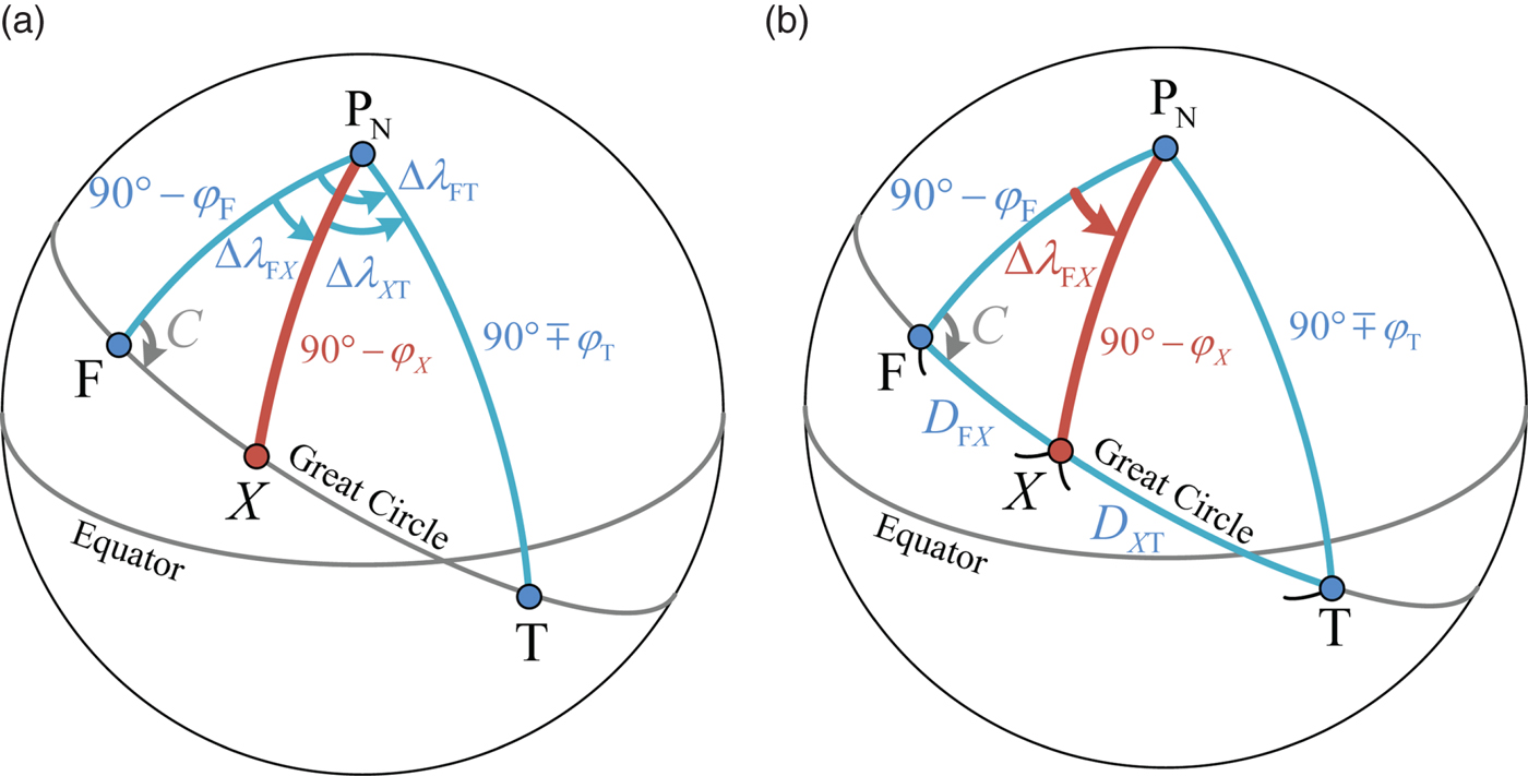
Figure 4. Finding the waypoints on the great circle track.
In the first given condition, by using Equation (3) we can directly obtain the latitude of the waypoint (φ X):
 $$\tan\varphi_{X}=\displaystyle{{\sin\Delta\lambda_{{\rm F}X}\tan\varphi_{\rm T}+\sin\Delta\lambda_{X{\rm T}}\tan\varphi_{\rm F}}\over{\sin\Delta\lambda_{\rm FT}}} $$
In the second given condition, by using Equation (6) we can directly obtain the latitude of the waypoint (φ X):
 $$\sin\varphi_{X}=\displaystyle{{\sin D_{{\rm F}X}\sin\varphi_{\rm T}+\sin D_{X{\rm T}}\sin\varphi_{\rm F}}\over{\sin D_{\rm FT}}} $$
Then, the difference of longitude between the departure point and the waypoint (Δ λ FX) can be obtained by using the law of cosines, and it can be converted into the longitude of the waypoint (λ X).
 $$\cos\Delta\lambda_{{\rm F}X}=\displaystyle{{\cos D_{{\rm F} X}-\sin\varphi_{{\rm F}}\sin\varphi_{X}}\over{\cos\varphi_{{\rm F}}\cos\varphi_{X}}} $$
We now take a practical example to demonstrate how to use the proposed formulae to find the waypoints on the great circle track. A ship is proceeding from Cape Town (33°53·3′S, 18°23·1′E) to New York (40°27·1′N, 73°49·4′W). In the first given condition, the difference of longitude between the departure point and the waypoint (Δ λ FX) is given (the value is 8°23·1′). In the second given condition, the great circle distance from the departure point to destination point (D FT) and the great circle distance from the departure point to the waypoint (D FX) are given (the values are 6,762.7 and 600 nautical miles). As shown in Table 1, using Equations (17), (18) and (19), we can respectively find the positions of the waypoints (X) in two kinds of given conditions.
Table 1. Results of calculating waypoints by using the formulae of the divided spherical triangle.

In fact, a number of recent textbooks adopt the formulae of the right spherical triangle to obtain waypoints on the great circle track (Bowditch, Reference Bowditch2017; Cutler, Reference Cutler2004; Royal Navy, 2008). This method is called the indirect approach because the position of the vertex must be found in advance. Although the follow-up studies claim that some new formulae which they proposed are the direct approach, they still have to calculate the initial great circle course angle (C) first (Chen, Reference Chen2016; Chen et al., Reference Chen, Hsieh and Hsu2015; Reference Chen, Liu and Gong2014; Nastro and Tancredi, Reference Nastro and Tancredi2010). In contrast, using the formulae of the divided spherical triangle can directly yield waypoints without calculating the initial great circle course angle (C). Some great circle track studies have also presented this type of method (Holm, Reference Holm1972; Miller et al., Reference Miller, Moskowitz and Simmen1991; Tseng and Chang, Reference Tseng and Chang2014).
4.2. Finding the astronomical vessel position of two celestial bodies
When the geographical positions and the observed altitudes of two celestial bodies are known, the main issue of the astronomical vessel position is to obtain the observer's position. Since the two circles of equal altitude may have two intersections, the obtained two possible positions of the observer need to be further judged to find the real astronomical vessel position. The judgement can be done through using the dead reckoning position. As shown in Figure 5(a) and Figure 5(b), the declination of two celestial bodies (d A, d B), the difference of hour angle between two celestial bodies (HA), and the observed altitude of two celestial bodies (H A, H B) are given to find the two possible positions of the observer (P1, P2), which include the latitude (L 1, L 2) and the meridian angle (t 1, t 2). Using the formulae of the spherical quadrilateral which was proposed in Section 3, this problem can be dealt with using the following steps.
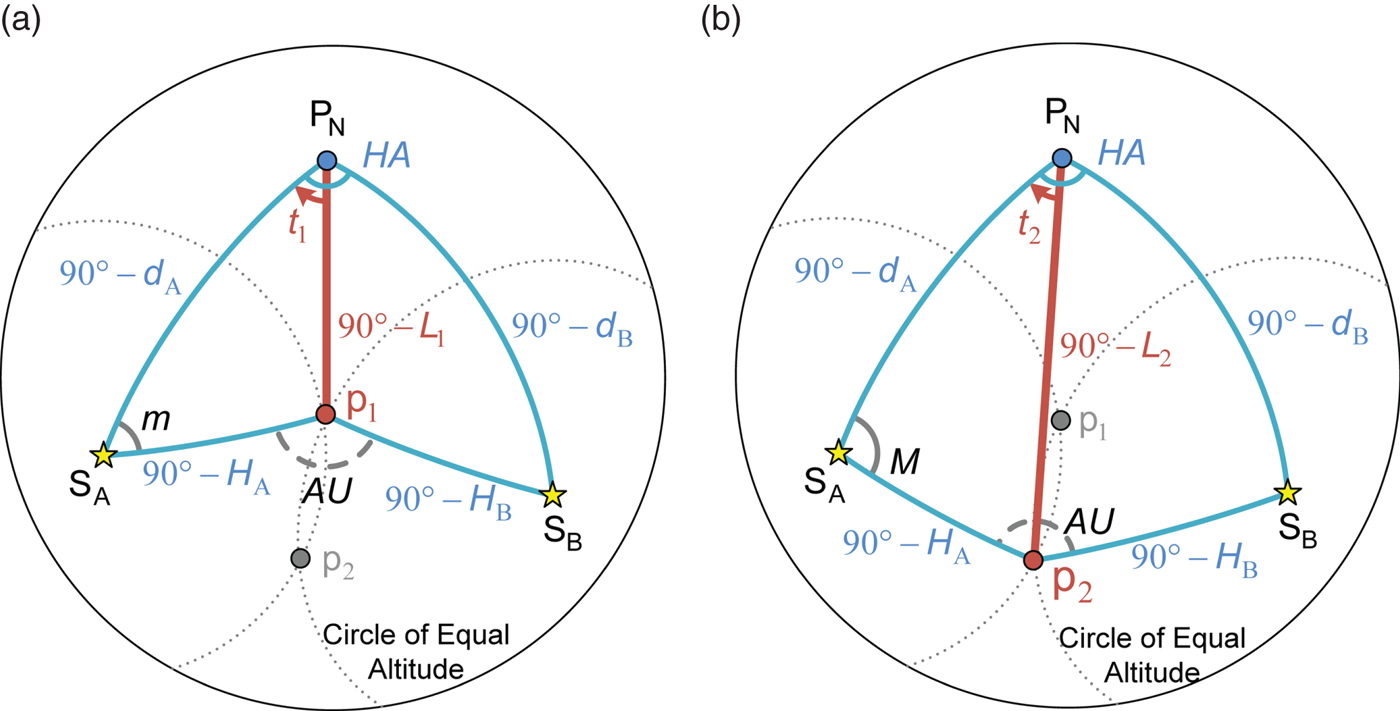
Figure 5. Finding the astronomical vessel position of two celestial bodies.
First, use Equation (9) to obtain the auxiliary angle (AU):
 $$\cos AU=\displaystyle{{\sin d_{\rm A}\sin d_{\rm B}-\sin H_{\rm A}\sin H_{\rm B}+\cos d_{\rm A}\cos d_{\rm B}\cos HA}\over{\cos H_{\rm A}\cos H_{\rm B}}} $$
where AU is the auxiliary angle, d A is the declination of celestial body A, d B is the declination of celestial body B, H A is the observed altitude of celestial body A, H B is the observed altitude of celestial body B and HA is the difference of hour angle between two celestial bodies.
Next, by using Equation (12), we can obtain the parallactic angle (m) in Figure 5(a):
 $$\tan m=\displaystyle{{\sin HA\lpar \cos H_{\rm A}\tan H_{\rm B}-\sin H_{\rm A}\cos AU\rpar -\sin AU\lpar \cos d_{\rm A}\tan d_{\rm B}-\sin d_{\rm A}\cos HA\rpar }\over{\lpar \cos d_{\rm A}\tan d_{\rm B}-\sin d_{\rm A}\cos HA\rpar \lpar \cos H_{\rm A}\tan H_{\rm B}-\sin H_{\rm A}\cos AU\rpar +\sin HA\sin AU}} $$
When the parallactic angle (m) is obtained, the latitude (L 1) and the meridian angle (t 1) can be yielded by using the law of cosines for the sides and the four-part formulae respectively:
 $$\sin L_{1}=\sin d_{\rm A}\sin H_{\rm A}+\cos d_{\rm A}\cos H_{\rm A}\cos m $$
 $$\tan t_{1}=\displaystyle{{\sin m}\over{\cos d_{\rm A}\tan H_{\rm A}-\sin d_{\rm A}\cos m}} $$
Lastly, we use Equation (13) to obtain the parallactic angle (M) in Figure 5(b):
 $$\tan M=\displaystyle{{\sin HA\lpar \cos H_{\rm A}\tan H_{\rm B}-\sin H_{\rm A}\cos AU\rpar +\sin AU\lpar \cos d_{\rm A}\tan d_{\rm B}-\sin d_{\rm A}\cos HA\rpar }\over{\lpar \cos d_{\rm A}\tan d_{\rm B}-\sin d_{\rm A}\cos HA\rpar \lpar \cos H_{\rm A}\tan H_{\rm B}-\sin H_{\rm A}\cos AU\rpar -\sin HA\sin AU}} $$
When the parallactic angle (M) is obtained, the latitude (L 2) and the meridian angle (t 2) can also be obtained by using the following formulae:
 $$\sin L_{2}=\sin d_{\rm A}\sin H_{\rm A}+\cos d_{\rm A}\cos H_{\rm A}\cos M $$
 $$\tan t_{2}=\displaystyle{{\sin M}\over{\cos d_{\rm A}\tan H_{\rm A}-\sin d_{\rm A}\cos M}} $$
We now demonstrate how we use the proposed formulae to find the astronomical vessel position of two celestial bodies by taking a practical example. We use the stars Capella and Alkaid as the basis of observation. The geographical position of Capella is (45°58·4′N, 131°24·8′W), and its observed altitude is 15°19·3′. The geographical position of Alkaid is (49°25·7′N, 3°14·2′W), and its observed altitude is 77°34·9′. The dead reckoning position is (41°34·8′N, 017°00·5′W). As shown in Table 2, adopting Equations (20) to (26) can respectively find the two possible positions of the observer (P1, P2). The second possible position of the observer (P2) is the real astronomical vessel position because its position is nearer to the position of dead reckoning. It should be noted that due to the property of the tangent function, −θ should be replaced as 180° − θ in the calculation process when the meridian angle is negative (t = −θ).
Table 2. Results of calculating astronomical vessel position by using the formulae of the spherical quadrilateral

* tan( − θ) = tan(180° − θ)
In fact, to find the astronomical vessel position of two celestial bodies, many studies have provided different approaches, such as the spherical triangle method (Chiesa and Chiesa, Reference Chiesa and Chiesa1990; Gery, Reference Gery1997; Karl, Reference Karl2007; Pepperday, Reference Pepperday1992; Pierros, Reference Pierros2018), the simultaneous equal-altitude equation method (Hsu et al., Reference Hsu, Chen and Chang2005), the complex analysis method (Stuart, Reference Stuart2009) and the rectangular coordinate method (Van Allen, Reference Van Allen1981). Similarly, adopting the formulae of the spherical quadrilateral can also deal with this problem. The concept of the method we propose is easier to comprehend, and its calculation process is concise.
5. CONCLUSIONS
This paper proposes two types of formulae for combined spherical triangles, which are the formulae of the divided spherical triangle and the formulae of the spherical quadrilateral. By using the divided spherical triangle formulae, we can directly obtain the positions of the waypoints without the extra calculation of the initial great circle course angle. By using the spherical quadrilateral formulae to solve astronomical vessel position problems, we can easier comprehend the calculation process concept than with some other methods.
ACKNOWLEDGEMENTS
The research presented in this paper has been supported by the Young Teacher Training Program of Shanghai Municipal Education Commission (ZZHS18053), National Natural Science Foundation of China (51709167), Natural Science Foundation of Shanghai (18ZR1417100), Shanghai Pujiang Program (18PJD017), Shanghai Shuguang Plan Project (15SG44), and Shanghai Science and Technology Innovation Action Plan (18DZ1206101).


