1. INTRODUCTION
Applications in many fields have been developed for Autonomous Underwater Vehicles (AUVs) including underwater exploration, deep-sea surveying and the maintenance of underwater installations (Krieg and Mohseni, Reference Krieg and Mohseni2010; Blidberg, Reference Blidberg2001; Monroy et al., Reference Monroy, Campos and Torres2017; Joung et al., Reference Joung, Lee, Nho and Kim2009). However, the capabilities of a single AUV are limited because of the limited available energy. Therefore, AUV cooperative working systems have been widely considered. For a multi-AUV system, cooperative hunting is an interesting problem (Li et al., Reference Li, Pan, Hong and Li2009) and can be divided into three subtasks: searching for the targets, task allocation, and real-time path planning in a fast-changing environment until capture is achieved (Li et al., Reference Li, Pan and Hong2010).
Much work has been completed on the overall hunting problem. Yamaguchi (Reference Yamaguchi1998; Reference Yamaguchi1999) applied a feedback control law to control mobile robots to capture targets in a time-varying environment. However, this control law can become deadlocked in an environment with many variably shaped obstacles. Ishiwaka et al. (Reference Ishiwaka, Sato and Kakazu2003) studied the hunting problem and presented an algorithm based on Reinforcement Learning (RL). This algorithm can decide the hunter's action (speed and direction) to hunt for the evaders. Song et al. (Reference Song, Li, Li and Ma2015) studied the hunting behaviour of multiple robots and proposed a mathematical model. The output of this model was stable, but the chase process was not studied because it assumed that the robots complete hunting when all of them detect the target. Inspired by the good performance of the Bio-inspired Neural Network (BNN) model to solve real-time path planning problems in dynamic environments, Ni and Yang (Reference Ni and Yang2011) used the model for real-time hunting of multiple robots. This algorithm can successfully finish the hunting problem. The fault tolerance of the algorithm was also verified. However, it would appear that all the hunting robots move faster than the targets, which may not be practical in reality. More importantly, all the robots shared the neural activity to hunt for a target during the pursuit stage in the study. Since the underwater environment has severe communication limitations, the sharing and spreading of neural activity will take a considerable time and cause delays. Real-time hunting is very difficult with such delays.
All the studies mentioned above focus on the Two-Dimensional (2D) ground-hunting problem. Hunting in the underwater environment is not the same as hunting on the ground as it is a Three-Dimensional (3-D) environment and path planning for AUVs can require significant calculation time. Nguyen and Hopkin (Reference Nguyen and Hopkin2005) proposed the use of multiple AUVs for mine hunting and proposed a complete coverage approach. Although the approach is efficient, the targets were static and had no intelligence and are thus easier to catch. Later, Williams (Reference Williams2010) reduced the distance for the AUV to detect the mine based on probabilities. Zhu et al. (Reference Zhu, Lv, Cao and Yang2015) solved the multi-AUV cooperative hunting problem with a BNN model by sharing the neural activities. They proposed a method for assigning hunting tasks based on distance-based negotiation between AUVs, but sometimes this could encounter conflicts. To overcome the conflicts, Cao et al. (Reference Cao, Huang and Zhu2015) and Cao and Yu (Reference Cao and Yu2017) proposed a location forecasting method. Chen and Zhu (Reference Chen and Zhu2018) solved the hunting problem of inhomogeneous AUVs and focused on the task allocation step but did not fundamentally solve the weakness of the GBNN model. More recently, Ni et al. (Reference Ni, Yang, Wu and Fan2018) proposed an approach based on the spinal neural system to perform the hunting control of multiple heterogeneous AUVs. This algorithm applied a spinal neural system for heterogeneous AUVs to search for evading targets. However, in the rounding-up step, they introduced a genetic algorithm to assign directions for the AUVs. The genetic algorithm needs several iterations to generate near-optimal directions for the AUVs, which can cause time delays. However, all of these studies assume that hunting AUVs are much faster than targets, which will greatly reduce the difficulty of hunting. If there is not much difference between the speed of AUVs and targets, it may be difficult for an AUVs to follow a fast-moving target in such a dynamic environment. An approach to plan the paths for the robots to track the fast escaping target is vital in the control of multi-AUV hunting.
Some neural network models have been proposed and have proved efficient for path planning. Agreev (Reference Agreev1998) proposed a multi-layer and feed-forward neural network for path planning. Xia and Wang (Reference Xia and Wang2000) presented a recurrent neural network for shortest-path routing. Although both of these algorithms are efficient for path planning, they are only suitable for stationary environments. Inspired by Grossberg's shunting model (Grossberg, Reference Grossberg1988), Yang and Meng (Reference Yang and Meng2000; Reference Yang and Meng2001; Reference Yang and Meng2003) proposed a BNN model for real-time path planning in dynamic environments. It is suitable for a wide range of robots. To make the BNN model suitable for the path planning of AUVs, Ni et al. (Reference Ni, Wu, Shi and Yang2017) proposed an improved dynamic BNN model. Although the algorithm reduces computational complexity, it does not guarantee an optimal path for the AUV. Lebedev et al. (Reference Lebedev, Steil and Ritter2005) applied a dynamic wave expansion model for robot path planning in time-varying environments. Owing to only four adjacent neurons in the model, the robot can only move in four directions. Glasius et al. (Reference Glasius, Komoda and Gielen1994; Reference Glasius, Komoda and Gielen1995; Reference Glasius, Komoda and Gielen1996) proposed the discrete Glasius Bio-inspired Neural Network (GBNN) model for path planning in environments containing obstacles. It has been applied in path planning for AUVs (Zhu et al., Reference Zhu, Liu and Sun2017), but it has been reported that it has difficulty in dealing with real-time path planning in rapidly changing environments. In order to make the GBNN model work well in fast changing environments, this paper presents several technical improvements and demonstrates that the improved model is suitable for real-time hunting control.
This paper considers the multi-AUV cooperative hunting problem, in which evading targets have intelligence. When an intelligent target changes direction, the AUV must adjust strategy quickly to generate a real-time and effective route to chase the target. The contributions of the paper can be described as follows.
(1) An improved GBNN model is proposed to adapt to a rapidly changing environment. For real-time path planning, the algorithm needs to be computationally efficient to avoid time delays. The improved GBNN model can meet the requirements, which makes it unnecessary to share neural activity among AUVs. Every AUV has its own neural activity for a target and plans the path by itself.
(2) The improved GBNN model has good dynamic performance and is able to track fast moving targets.
(3) A novel dynamic alliance-forming strategy is proposed to distribute the hunting task for the AUVs. The strategy is suitable for both homogeneous and inhomogeneous AUVs. From simulation studies, it can be seen that both the proposed alliance-forming strategy and the improved GBNN model can successfully solve the hunting problem of multi-AUV systems.
The rest of this paper is organised as follows: Section 2 introduces the multi-AUV cooperative hunting problem. In Section 3, the algorithm to control multiple AUVs in cooperatively hunting for an intelligent evading target is proposed. In order to demonstrate the validity of the proposed algorithm, simulations are reported in Section 4. Finally, some conclusions and directions for possible future research are made in Section 5.
2. THE MULTI-AUV COOPERATIVE HUNTING PROBLEM
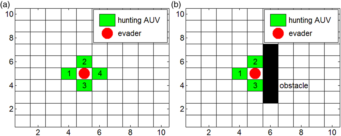
As a grid map simplifies the problem and is convenient for study of hunting, it is applied in this study. At first, a set of AUVs are to hunt for several evading targets. It is supposed that n AUVs (AUV1, AUV2, …, AUVn) are to hunt for m evaders (Ev1, Ev2, …, Evm). To catch the evader, hunting AUVs in a hunting alliance move towards the evader. When the AUVs tightly encircle and evenly distribute around the evader, hunting succeeds. As shown in Figure 1, the black blocks represent obstacles and the blank areas are the free spaces. Four hunting AUVs are required in a 2D environment to encircle an evader, and six AUVs are required to form a successful encirclement in 3-D hunting. If any obstacle helps with the successful capture, the hunting can be successful with fewer AUVs, as shown in Figure 1(b).

Figure 1. Illustration of successful hunting in a 2-D environment.
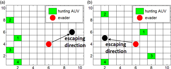
An intelligent evader can run to avoid being caught. Their evasion strategies can be divided into two different situations as shown in Figure 2. When the surrounding encirclement has not formed as shown in Figure 2(a), the evader travels away from the AUVs to prevent being caught. The evader changes its direction by changing its target point as in:

Figure 2. Evasion strategies in a 2-D environment.
 $$e_t =e_c +\sum_{i=1}^n (e_c -w_i) /r $$
e t is the location of the evader's target point which will make it run against the hunting AUVs. e c means its current position, and n is the quantity of AUVs within the perception region. w i is the position of AUVs near the evader where n evaders are assumed to be nearby. r > 1 is introduced to avoid the coordinates of its target from exceeding the size of the environment.
Another situation is that the AUVs are distributed around the evader. In this situation, the evader should run to the mid-point of the two AUVs furthest away, as shown in Figure 2(b).
In the 3D environment, the surrounding encirclement is examined through projection. We can take every one of the three coordinate planes to examine the encirclement. If no encirclement is formed in any of the planes, a 3D encirclement is not formed. Similarly, if no surrounding encirclement is formed, the evader moves away from the AUVs; otherwise, the mid-point between two farthest adjacent AUVs will be the escape direction.
An evader's escaping strategy in these two situations are consistent with the general situations. In practical applications, the evader usually moves to keep away from the AUVs. Our strategies can help the evader to find a direction with the highest opportunity to escape from being hunted. Since the intelligent evader applies the proposed escaping strategies, which lets it possess the ability to avoid being hunted, it is harder for the AUVs to encircle the evader. The escaping strategies are proposed for general cases and are independent of the proposed hunting algorithm.
3. PROPOSED STRATEGIES
This study proposes strategies for allocating the hunting mission to form effective hunting alliances and real-time path planning to capture fast escaping evaders.
3.1. AUVs' dynamic alliances
To make an easy calculation, the locations of evaders are programmed into the matrix E, and the matrix W represents the locations of AUVs. Each row of the two matrices is their coordinate value.
 $$E=\left[\matrix{ x_1 & y_1 & z_1 \cr \vdots & \vdots & \vdots \cr x_m & y_m & z_m \cr}\right]$$
 $$W=\left[\matrix{ w_{1x} & w_{1y} & w_{1z} \cr \vdots &\vdots & \vdots \cr w_{nx} & w_{ny} & w_{nz} \cr}\right]$$
 $$D_{we} := \sqrt{W_.^2 \cdot M_1 +M_2 \cdot ( E^{\rm T}) _.^2-2\cdot W\cdot E^{\rm T}} $$
In Equation (4), M 1 is a 3* m matrix, and the size of M 2 is n* 3. The values of all the elements of matrices M 1 and M 2 are one. E T is the transpose of E. D we is an n* m matrix, and the j-th column contains the distances from the evader j to the AUVs from 1 to n.
Inhomogeneous AUVs possess distinct energies and thrust torques. They have different safety distances and maximum sailing speeds. The safety distance for an AUV is the total distance it can run without worrying about having insufficient energy. If d wiej exceeds the AUV's sailing capability, it is simply set to infinite.
 $$d_{wiej}=\left\{\matrix{ d_{wiej}\comma \; & d_{wiej} \le c_{safei} \hfill \cr \infty\comma \; & else \hfill \cr}\right. $$
 $$t_{we}:= ( D_{we}) ./Spd $$
In Equation (5), d wiej is the element of D we in row i and column j. c safei is defined as the i-th AUV's safety distance. The estimated hunting time is acquired from Equation (6). Spd contains the velocity values of every AUV, which is programmed to be the same size as D we. The elements of its row vector are the velocity values of the AUVs.
With t we, dynamic hunting alliances between AUVs using Algorithm 1 are formed. The inputs of the algorithm contain t we: estimated hunting time matrix; TeamNum: The maximum number of hunting teams that can be formed by AUVs; Num: number of AUVs required, for 2D encircling it is four, for 3D encircling it is six; NumEvader: evaders' number to be hunted. The outputs of the algorithm are the evaders' hunting order (evIndex: row vector); the index of AUVs in each of the hunting alliance (auvIndex: matrix).
ALGORITHM 1
Step 1: Initialise: set j = 1, evIndex = a zero vector (1*TeamNum), and auvIndex = a zero matrix (TeamNum* Num);
Step 2: LOOP: sort t we: [stT, winners = Sort(twe);
Step 3: For each evader, get the first Num rows of stT: For i = 1 to NumEvader: tmSdT(:,i) = stT(1:Num,i);
Step 4: Sum and sort tmSdT: tmTotTime = sum(tmSdT), [,winnerIndex = sort (tmTotTime);
Step 5: Get the index of the most easily caught evader: evIndex(1,j) = winnerIndex(1,1);
Step 6: Assign the AUV that has no hunting task and can reach the evader with the minimum estimated time to hunt for the evader: auvIndex(j,:) = winners (1:Num,evIndex(1,j));
Step 7: Set the arrival time to a large positive value to prevent the evader from winning the competition again: t we (:,evIndex(1,j)) = colBigValue;
Step 8: j increases by 1: j = j + 1;
Step 9: return to LOOP until the condition (j ≤ NumEvader & j ≤ TeamNum) is not satisfied.
In our strategy, the AUVs first hunt for the easiest evader who has the least estimated hunting time. After the evaders' hunting sequence is determined, the AUVs with the least total hunting time for an evader will form a hunting alliance. The alliance is dynamic as the environment changes. In the alliance formation mechanism, we consider AUVs' different speeds, which makes the hunting faster with less chasing and gives a shorter evading distance.
3.2. Distribution of hunting points
The AUVs must occupy the hunting points around the evader to complete the hunting task. If the AUVs do not form an encirclement, then the strategy assigns the nearest and fastest AUV in the hunting alliance to move to the other side to hinder the escape of the evader, as shown in Figure 3(a). When the AUVs have formed a surrounding encirclement, then the strategy first allocates the easiest point that is nearest to one of the AUVs, and this easiest point is assigned to the nearest AUV on the evader's same side, as shown in Figure 3(b).
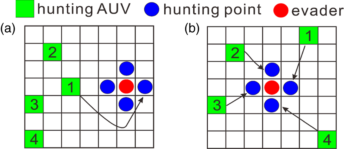
Figure 3. Distribution of hunting points.
The hunting point distribution strategies help to define clear target points for every AUV. Without any conflict among AUVs, they quickly move closer to the evader. The distribution strategies can also prevent the evader from escaping since the strategies can control the AUVs to quickly form an encirclement. Although the evader is intelligent, and the hunting is hard, the hunting point distribution strategies proposed for the general cases help to improve hunting efficiency.
3.3. Improved Glasius Bio-inspired Neural Network
After the AUVs form a hunting group and hunting points are distributed to them as their target points, path planning to the assigned points is the next step.
3.3.1. Review of Glasius Bio-inspired Neural Network
Glasius et al. (Reference Glasius, Komoda and Gielen1996) proposed the Glasius Bio-inspired Neural Network (GBNN) model. The models for 2D and 3D environments are shown in Figure 4. A neuron is connected with its neighbours. The model is described in Equation (7).
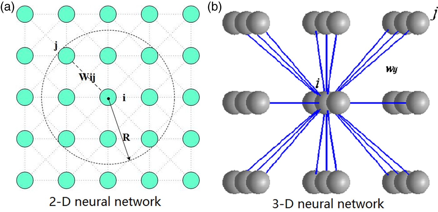
Figure 4. GBNN neural network.
 $$x_i( t+1) = f\left(\sum_{j \in S_i} ( w_{ij}\cdot x_j( t) ) +I_i\right)$$
 $$w_{ij}=\left\{\matrix{e^{-\gamma \cdot dist( p_i-p_j) } & \hbox{if}\, dist( p_i-p_j) \le R \hfill \cr 0, \; & \hbox{otherwise} \hfill \cr }\right. $$
 $$I_i=\left\{\matrix{v\comma \; & \hbox{grid}\; i \; \hbox{is target} \hfill \cr -v\comma \; & \hbox{grid}\; i\; \hbox{is occupied} \hfill \cr 0\comma \; & \hbox{else}}\right. $$
 $$f( x) =\left\{\matrix{1\comma \; & x \ge 1 \hfill \cr \beta \cdot x\comma \; & 0 \lt x \lt 1 \hfill \cr 0\comma \; & \hbox{else} \hfill \cr }\right. $$
 x i (t + 1) is the i-th grid's neural activity at the current time step. x j (t) is the neighbour's neural activity a time step before the current time step. w ij means the weight value to connect the neurons, and  $dist( p_{i} -p_{j}) $ represents the neurons' Euclidean distance. R is the radius as shown in Figure 4. I i is the external input value representing the information of each grid, and v > >1. The occupied grids mean that other AUVs, obstacles, mountains, or evaders are located at the grids. f(x) in Equation (10) is a transfer function, which is piecewise and linear.
There are two main parameters, γ and β, in the GBNN model. The choice of γ and β needs to ensure neurons other than the target neuron have an activity level less than one. For 2D application, R is usually equal to  $\sqrt 2 $, the constraints are described by Equation (11):
 $$\left\{\matrix{ 4 \cdot \beta \cdot ( e^{-\gamma} + e^{-2\gamma}) \lt 1 \hfill \cr 4( e^{-\gamma} + e^{-2\gamma }) \lt 1 \hfill \cr }\right. $$
 If β is equal to 1, the upper inequality in Equation (11) is the same as the second one and then  $\gamma \gt ( \ln ( 2\sqrt 2 +2) \approx 1.5745) $. Since the parameters are limited, the GBNN model has dissatisfactory decay rates. The GBNN model has a fixed decay rate in the time dimension, which is equal to one. This makes it possible that the change of neural activity lags behind the fast-changing environment. In the space dimension, however, the GBNN model has an exponential decay rate which decays quickly. It takes some time steps for the propagation of a target's neural activity to reach the AUV's initial position. With the time steps delay, the GBNN model is also unsuitable for real-time path planning.
3.3.2. Improved Glasius bio-inspired neural network
Some technical improvements are proposed to give the GBNN model a better performance in real-time path planning in a dynamic environment.
First, it is necessary for the neural activity to spread fast in the environment for real-time path planning. For the fast propagation of neural activity over the whole environment in a time step, we have to calculate the neural activity of the GBNN model outwardly from the target neuron, which can be referred to as a backward calculation as shown in Figure 5. The yellow circle represents the target neuron and its activity is calculated first. Activity of neurons a grid next to the target is calculated next and other neural activity is obtained sequentially as grids extend out.
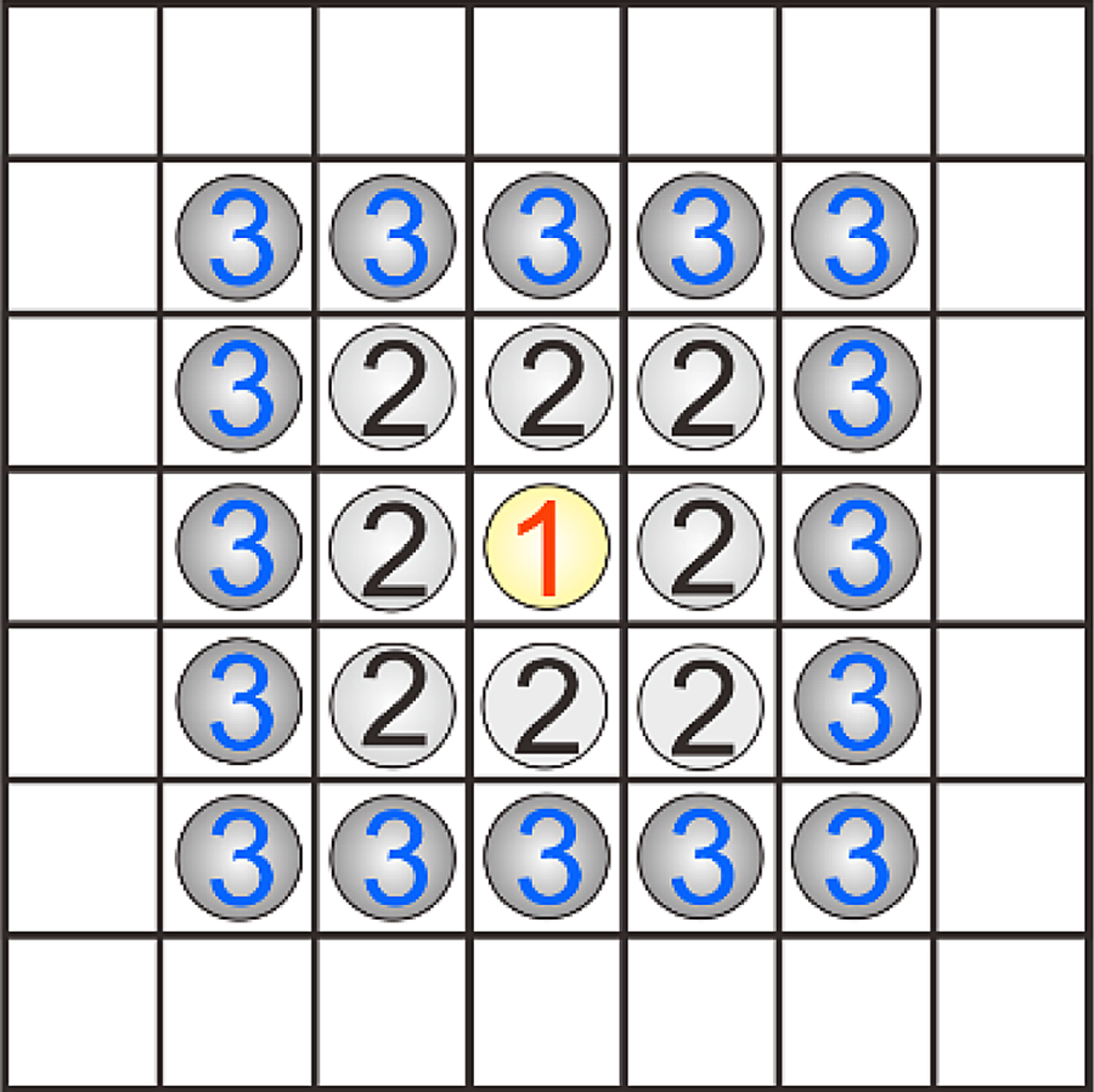
Figure 5. Backward calculation from target neuron (numbered “1”).
Second, the neural activity contains incorrect path information when the target or obstacle moves quickly in a dynamic environment. When the target or obstacle moves quickly, all the neurons are suppressed at the next time step and the neural activity is recalculated outwardly starting from the target position.
Third, the model can be improved to achieve higher decay rate in the time dimension, which is described in Equation (12):
 $$x_i( t+1) = f\!\!\left(\sum_{j \in S_i} ( w_{ij} \cdot x_j( t) ) + I_i - R^2 \cdot e^{-\gamma \cdot R^2} \cdot x_i( t) \right)$$
Equation (12) is the same as Equation (7) apart from an added decay term. All symbols have the same meanings as described in Equations (7)–(10). With this model, the constraints of the parameters are described by Equation (13) for a 2D environment.
 $$\left\{\matrix{ \beta \cdot ( 4 \cdot e^{-\gamma} + 2 \cdot e^{-2\gamma}) \lt 1 \cr 4 \cdot e^{-\gamma} + 2 \cdot e^{-2\gamma} \lt 1 }\right. $$
 If β is equal to 1, then  $\gamma \gt ( \ln ( \sqrt{1.5}-1) \approx 1.4928) $. With the improvements, properties as follows can be obtained:
Property 1. With the neural activity calculated outwardly from the target location, neurons in the grid map can be active in a time step. The model can be applied in real-time path planning without any delay in the propagation of neural activity.
Property 2. The additional decay term can enhance neuronal dynamic performance in the time dimension and helps to slightly improve parameter performance since the value of γ can be reduced. Moreover, neurons are suppressed when the environment changes quickly, which helps to reduce the cumulative error message of the path. When the neural activity changes as fast as the time varying environment, it is suitable for path planning in a fast-varying environment.
Property 3. With the additional decay term, the model is still stably calculated. The added decay term makes the time decay rate of the GBNN model higher than 1, which is  $1+e^{-\gamma \cdot R^{2}}$. The higher decay rate allows the neuronal activity to stabilise more quickly. In fact, because a decay term is added, it shortens the time for the system to reach the equilibrium state.
3.3.3. Path Planning
With the improved GBNN model, the AUV sails to the grid next to the AUV's current position, which has the greatest neural activity.
 $$Path=P_n \vert x_{P_n } =\max \lcub x_i \comma \; i=1\comma \; 2\comma \; \ldots\comma \; k\rcub \comma \; P_p =P_c \comma \; P_c =P_n $$
x i is the grid's activity near the AUV's current position. For the 2D environment, k is set to 8, and it is set to 26 in the 3D environment. P p, P c and P n are positions of the AUV at three adjacent time steps.
The improved algorithm with fixed calculation direction accelerates the propagation of neural activity. The additional decay item also improves the dynamic property of the GBNN model. Even if the evader keeps escaping, this approach ensures the obstacle grid has minimal neural activity and changes the neural activity as fast as the changing environment.
4. SIMULATION STUDIES
In order to study the feasibility of hunting control by the proposed strategies, several simulation experiments were conducted using MATLAB. We made three reasonable assumptions for the convenience of the simulation experiments. First, since the ocean environment is vast, the shapes of the evader and the AUV were ignored. The evader and the AUV are worked as mass points. Second, it is supposed that an AUV can turn its direction slowly to track the path planned by the improved GBNN model. The speed of an AUV is usually slow. This assumption is reasonable as an AUV has plenty of time to change its direction to follow the planned path. Third, the location information of the evader is known to the AUVs after one of the AUVs finds it. In fact, the location information of the evader is a short message, and it can be transmitted to the AUVs quickly. The neural activities around the environment do not need to be propagated, which makes communication quick enough to spread the location information of the evader. Experiments of 2D hunting control are described first. The results are compared with algorithms such as a BNN model and distance-based hunting alliance strategies. Finally, a 3D cooperative hunting experiment was also devised. In the simulation experiments, the size of obstacles was expanded to avoid AUV collisions under actual conditions. The enlarged grids are marked as grey units. The simulation programs run on a computer with an i7-6700HQ Core and 16 GB memory.
4.1. Hunting in a 2D environment
In a 2-D environment, eight AUVs need to hunt for two evaders. The size of the designed hunting environment contains 60*60 grids. The perception range of the evader is a circle with a diameter of ten grid units, and it runs away from the AUVs when it detects hunting AUVs nearby. First, a simulation experiment was devised that all AUVs are twice as fast as the evaders. The hunting task was fulfilled with the improved GBNN model and the BNN model, respectively. After that, as in our lab, some AUVs are slower than others, and may only have the same speed capability as the evader. For the same environment, the experiment of hunting by inhomogeneous AUVs with different speed capabilities is to verify the validity of the proposed alliance formation mechanism. In order to make the simulation experiment more in line with the real world, multi-threading technology was used to complete an independent calculation of the neural activity of each AUV.
4.1.1. Hunting of homogeneous AUVs with the proposed algorithm
Initially, two evaders were located at grids (6, 15) and (56, 54), and moved randomly. Eight AUVs were at the boundary of the environment and were ready for hunting. In this section, it is supposed that all AUVs are twice as fast as the evaders. The parameters are set as β = 1, v = 200,  $\gamma =1.4929$ and
  $R=\sqrt{2}$. For all the 2D hunting experiments with the improved GBNN model, parameters are all set with the same values. The hunting process is shown in Figure 6. In the figure, the black blocks represent obstacles, the symbols of different shapes and colours represent different AUVs and the evaders are represented by the red circles. The hunting step count increases after each evader's movement.

Figure 6. Result of hunting by homogeneous AUVs with the proposed algorithm.
Figure 6 shows that eight AUVs form two hunting alliances. A team comprising AUV1, AUV2, AUV7 and AUV8 hunted for Ev1. Another group pursued Ev2. The intelligent evaders ran in the opposite direction to the AUVs to escape from being hunted when they detected the hunting AUVs. AUV7 encountered an obstacle at grid (2, 57), and it avoided the obstacle with the improved GBNN model. Moreover, with the improved GBNN model, the AUVs got closer to their hunting points to fulfil the hunting mission. Ev1 and Ev2 were encircled at grids (8, 29) and (57, 45) respectively. The program ran for 40 hunting steps. The second column of Table 1 lists the AUVs' distance cost and the evaders' escaping distance.
Table 1. Comparison of hunting simulations by improved GBNN and BNN models

4.1.2. Hunting of homogeneous AUVs with BNN model
For the same situation stated above, the BNN model was applied for path planning. For full access to the BNN model compared, see Yang et al. (2001, 2000, 2003). In the BNN model, the parameters were set as follows in the simulation, B = D = 1, A = 25, u = 1 and R = 2. Figure 7 shows the hunting result. The AUVs were similarly distributed and constructed the same hunting alliances. Hunting was completed with the BNN model but took more steps and much more running time. Ev1 and Ev2 were encircled at grids (13, 32) and (57, 52), and the program ran for 45 hunting steps. Ev2 ran further as AUV6 occupied the hunting point later than in the GBNN model. This was the same for Ev1. The third column of Table 1 lists the AUVs' distance cost and the evaders' escaping distance for comparison.
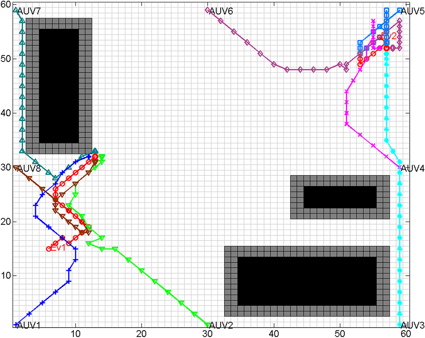
Figure 7. Result of hunting by homogeneous AUVs with BNN model.
With the improved GBNN model, the AUVs finished hunting with an average distance travelled of 3,772 m, and that of BNN model is higher. The BNN model has been reported as suitable for real-time path planning. Nevertheless, the improved GBNN model provides the AUV with a more direct direction and a shorter path. The technical improvements to the GBNN model improve its dynamic performance to provide effective path information. More importantly, the improved GBNN model does not cost much computation time, requiring only 2.9 seconds of simulation time. The BNN model needs to solve a differential equation for each neuron and takes 311.2 seconds for the same process. In the experiments, except for the calculation of neural activity, the other procedures are the same. In this regard, the BNN model is very time consuming and will be unmanageable in a 3D underwater environment, where many neurons are required to construct the environment. Therefore, the improved GBNN has a good performance in real-time path planning in fast changing environments and is computationally efficient.
4.1.3. Monte-Carlo hunting simulations by homogeneous AUVs with the GBNN and BNN models
In the 2D environment, the locations of the evaders were randomly generated 50 times in performing Monte-Carlo tests. Both the GBNN and BNN models were applied to fulfil the hunting task for comparison. After the simulation experiments, the average distance the AUVs and evaders travelled was calculated. Meanwhile, the average simulation time is also listed, as shown in Table 2. In the experiments, the result of the path planning method using the BNN model is inferior to the improved GBNN method. With the improved GBNN model, the average travelled distance of the AUVs was 3,795 m, whereas for the BNN model, it was 4,058 m. In addition, the BNN model took 308.6 seconds on average to complete an experiment, which is much higher than the improved GBNN model. The high computational complexity may make it impossible for the BNN model to satisfy the requirements of real-time path planning. However, the improved GBNN model can have a good dynamic performance while ensuring low computational complexity.
Table 2. Average cost and efficiency comparison of 50 repetitions of Monte-Carlo simulations
4.1.4. Hunting of inhomogeneous AUVs by the proposed time-based alliance formation mechanism
Hunting experiments of multiple inhomogeneous AUVs with different speed capabilities were performed for the same hunting task as described above. AUV1, AUV3, AUV5 and AUV7 have the same speed capability as the evaders, and others can run at double the speed of the evaders. The experiment was first carried out with the proposed alliance formation mechanism and the improved GBNN model. As shown in Figure 8, the hunting process is longer than the previous experiment as not all the AUVs are running faster than evaders.
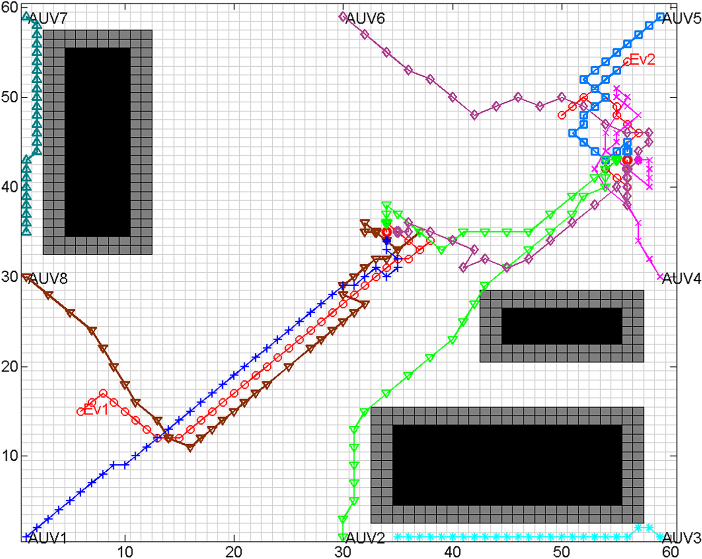
Figure 8. Result of hunting by inhomogeneous AUVs with the proposed algorithm.
At first, AUV1, AUV3, AUV7 and AUV8 were distributed to hunt for Ev1. The rest of the AUVs were allocated to pursue Ev2. As the team to hunt for Ev2 had a high-speed capability, Ev2 was quickly encircled at grid (56, 43). After that, the alliance to chase Ev1 changed. AUV2 and AUV4 replaced AUV3 and AUV7, and the hunting for Ev1 was finished at grid (34, 35). The program ran for 62 hunting steps. The second column of Table 3 lists the distance travelled for each AUVs and the evaders' escaping distances.
Table 3. Comparison of hunting simulations by different alliance formation methods

4.1.5. Hunting of inhomogeneous AUVs by distance-based alliance
In the distance-based strategy, AUVs negotiate to form hunting alliances with neighbour rules. For a full access to the strategy, See Zhu et al. (Reference Zhu, Lv, Cao and Yang2015). The result of hunting with the distance-based alliance formation method is shown in Figure 9. The AUVs construct different dynamic hunting alliances. AUV1, AUV2, AUV7 and AUV8 hunted for Ev1. The remaining AUVs chased Ev2. The hunting was completed with this alliance formation algorithm but requires much longer chasing distances. Ev1 and Ev2 were encircled at grids (31, 4) and (3, 5) respectively. The program ran for 138 hunting steps. As the hunting alliance is formed by negotiation that only depends on the position information of AUVs and evaders, one of the AUVs may have a low speed, resulting in a low chasing efficiency. The third column of Table 3 lists the distance cost of AUVs and the escaping distance of evaders to make a comparison.
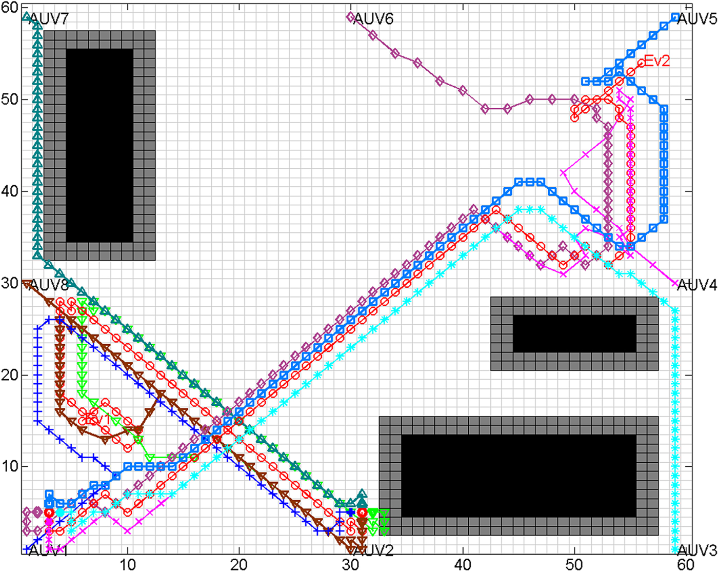
Figure 9. Result of hunting by inhomogeneous AUVs with distance-based mechanism.
With the time-based alliance formation mechanism, the AUVs finish hunting with an average distance of 5,055 m, but the distance-based mechanism requires 9,466 m. The dynamic hunting alliances constructed with the time-based alliance formation mechanism can take advantage of each AUV, which will improve the hunting efficiency and cut down the hunting cost. In other words, the proposed strategies set up the hunting alliances that allow a hunting group to have almost the same AUVs with the same speed abilities. The distance-based negotiations ignore the speed capabilities of the AUVs, and the capability of a hunting group is limited by the weakest AUV. The distance-based negotiation cannot solve the problem of hunting task allocation of multiple AUVs with different abilities. The time-based alliance formation mechanism is more efficient and effectively assigns the hunting task among multiple AUVs.
4.2. Simulation design of hunting in a 3D environment
The underwater environment is a Three-Dimensional (3D) and obstacle cluttered environment. A 3D environment for the hunting simulation experiment was designed. Mountains exist at the bottom as shown in Figure 10. As shown in Figure 10, the coordinate “0” of the “z” axis is set as zero metres. Taking this as a reference, the height of the valley is −1,500 m, and the height of the mountain is 2,000 m. The hunting AUVs are located in the eight corners of the simulated environment. An evader is initially located in the middle, at grid (20, 30, 34). In the experiment, AUV3, AUV5, AUV6 and AUV7 had the same maximum speed as the evader, and the others had double the speed of the evader.
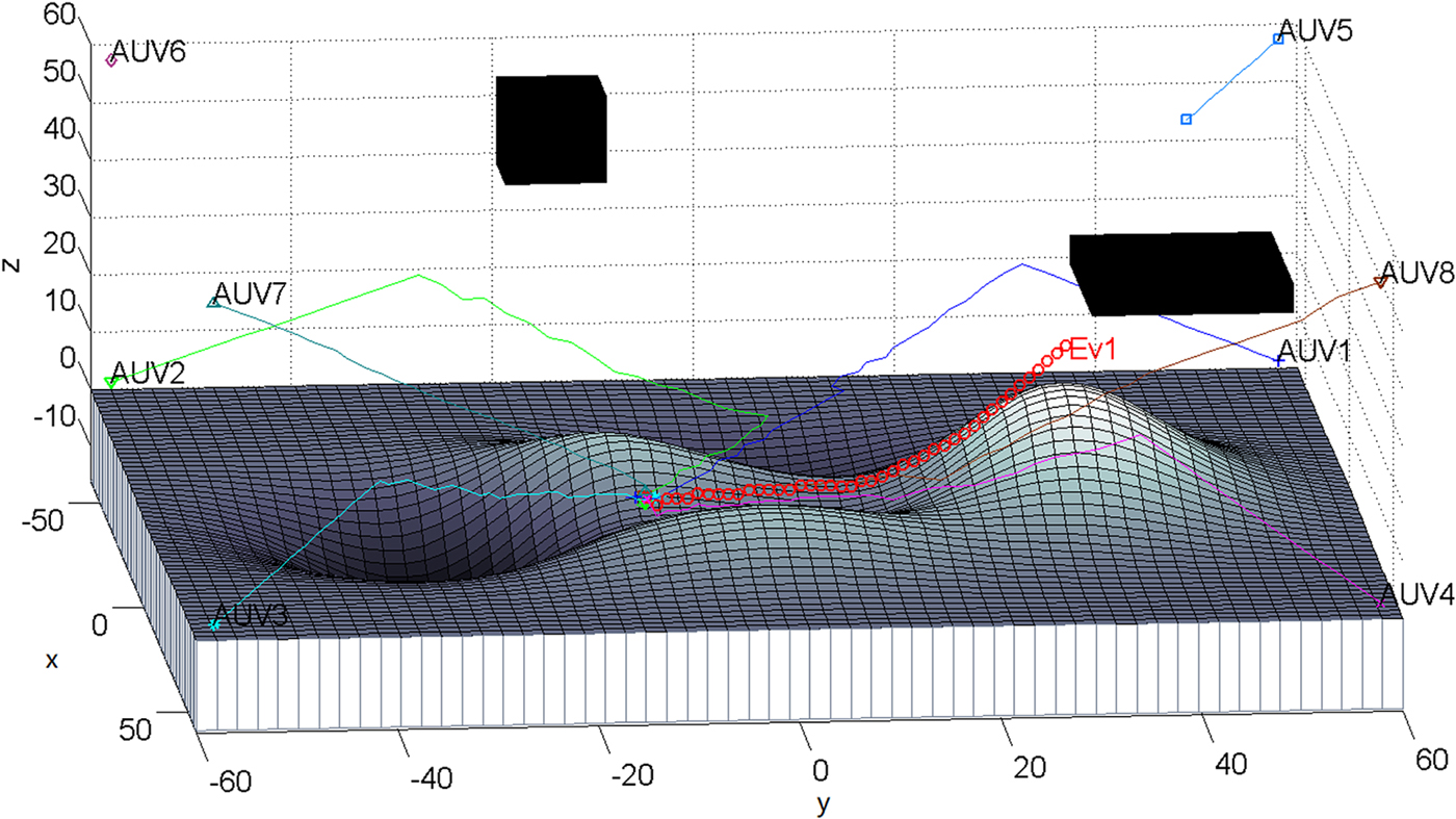
Figure 10. PUnderwater hunting with improved GBNN model, view from grid (85, 30).
For the application of the improved GBNN model in a 3D environment, R is equal to  $\sqrt{3}$, then γ and β are subjected to the constraint of Equation (15).
 $$\left\{\matrix{ ( 6 \cdot e^{-\gamma } + 12 \cdot e^{-2\gamma } + 5 \cdot e^{-3\gamma}) \cdot \beta \lt 1 \hfill \cr 6 \cdot e^{-\gamma } + 12 \cdot e^{-2\gamma } + 5 \cdot e^{-3\gamma } \lt 1 \hfill \cr}\right. $$
 If β is equal to 1, then  $\gamma \gt( \ln ( \displaystyle{{\sqrt {69} +7}\over{2}}) \approx 2.0351) $. Therefore, in the experiment, β = 1, v = 200,
  $\gamma =2.0352$ and
  $R=\sqrt 3 $.
Figure 10 shows the hunting process of this experiment from the viewpoint at grid (85, 30). The hunting task was first assigned to AUV1, AUV2, AUV4, AUV5, AUV7 and AUV8. As the evader goes nearer to AUV3 while it is escaping, which makes the distance from the evader to the AUV5 further than the distance from the evader to AUV3, AUV5 is replaced by AUV3 at the tenth hunting step. In the hunting process, the AUVs are able to prevent collision with hills and obstacles and change their directions as soon as the evader runs to another location. AUV5 sailed a distance of 1,732 m and then stops at grid (−48, 48, 48). The distances that AUV1, AUV2, AUV3, AUV4, AUV7 and AUV8 travelled are 12,678, 12,932, 7,368, 9,274, 7,781 and 10,445 m, respectively. The evader was encircled in a globe by six AUVs at grid (22, −19, 8) with the escaping distance travelled of 7,923 m. The program ran for 59 hunting steps and took 798.6 seconds. With the improved GBNN model, the AUVs updated their neural activity in 13.5 seconds. The BNN model was also tested for path planning in the vast 3D environment, and the program took more than two hours to update all the neural activities of the grids in the environment. This is not practical for 3D real-time hunting applications.
5. CONCLUSION
The study described in this paper researched a multi-AUV cooperative hunting problem, and it mainly focused on the final two steps. The algorithm formed effective hunting alliances, dividing the AUVs into groups and chasing the evaders one by one. The mechanism can work well for both homogeneous and inhomogeneous AUVs. In addition, the GBNN model is improved for real-time path planning in a fast-changing environment. The effectiveness of the proposed algorithm has been demonstrated through analysis and simulation studies. The improved GBNN algorithm was compared with the BNN model. The strategies presented in the study reduced the chasing distances of AUVs. The simulation also shows that the algorithm successfully performs underwater hunting by multiple AUVs, in a three-dimensional and obstacle cluttered environment. The improved GBNN model, which is computationally efficient, is also suitable for hunting control in a 3D environment. In this research, the AUV is considered to be able to move quickly to follow up the path planned by the GBNN model. Although the AUV's speed is slow and it can theoretically track the path, trajectory tracking of the AUV needs to be further studied to demonstrate the assumptions proposed in this paper. Different from many studies where the path is usually pre-set in advance, trajectory tracking in the hunting control is a dynamic trajectory tracking where the trajectory is previously unknown.
ACKNOWLEDGEMENTS
This work was supported in part by the National Natural Science Foundation of China (U1706224, 91748117, 51575336), the National Key Project of Research and Development Program (2017YFC0306302), Creative Activity Plan for Science and Technology Commission of Shanghai (16550720200).