1. Introduction
One of the most important challenges associated with enabling world-wide commercial navigation relates to safety. Institutions, regulations and procedures have been developed over time to ensure safety at sea, which have considered ‘such desirable conditions of human activity at sea that do not endanger human life and property, and are not harmful to the maritime environment’ (Kopacz et al., Reference Kopacz, Morgaś and Urbański2001). Different scientific and technological advances have contributed to both economic feasibility and safety of maritime navigation. Particularly, fields such as electronics, radio, computer science, automatic control engineering, data presentation and space technologies have led to the development of integrated equipment and systems to assist in the ship's operation (Kopacz et al., Reference Kopacz, Morgaś and Urbański2004). Note that as the human activity at the sea increases, there is a corresponding need for general improvements in overall safety and efficiency of maritime operations. Further usability studies have been proposed towards the development of optimal user interfaces for maritime equipment (Hareide and Ostnes, Reference Hareide and Ostnes2017).
Technological trends, such as autonomous vehicles and robotics; artificial intelligence; big data; virtual, augmented and mixed reality; internet of things; cloud and edge computing; digital security; and three-dimensional printing and additive engineering, have recently been investigated towards improvements in the performance of existing maritime operations (Sanchez-Gonzalez et al., Reference Sanchez-Gonzalez, Díaz-Gutiérrez, Leo and Núñez-Rivas2019). The incorporation of new navigation-related technologies in maritime equipment is usually associated with an increase in the amount of information and alerts displayed (Maglić and Zec, Reference Maglić and Zec2020).
Tools with augmented reality (AR) methods have been proposed for presenting navigational data. Such tools may facilitate the interpretation of navigational information during operation. Holder and Pecota (Reference Holder and Pecota2011) conducted tests with full-mission simulations for the definition of operational requirements for a maritime head-up display (HUD) system. Alternative types of AR solutions (monitor augmented reality; MAR) uses a monitor for displaying navigational information (Morgère et al., Reference Morgère, Diguet and Laurent2014; Hong et al., Reference Hong, Andrew and Kenny2015; Oh et al., Reference Oh, Park and Kwon2016; Mihoc and Cater, Reference Mihoc and Cater2017). A systematic review regarding the use of augmented reality technology in the field of maritime navigation is presented by Laera et al. (Reference Laera, Fiorentino, Evangelista, Boccaccio, Manghisi, Gabbard and Foglia2021).
Usability and precision considerations regarding the full development of an operational MAR system are beyond the scope of the present work. Instead, a preliminary investigation is proposed towards the development of a MAR system for navigational assistance in restricted waters. In such a system, a monitor displays the scene measured by a camera that is rigidly attached to the ship. Virtual elements are rendered on top of the navigation scene to assist with their perception.
In the following section, foundations for augmented reality systems are briefly summarised. Next, the synthesis of virtual elements in maritime scenes is proposed with navigation experiments. The experiments assume that the camera is rigidly attached to the ship in a MAR setup. Finally, potential navigational assistance applications are discussed with examples of augmented scenes that combine pertinent virtual elements.
2. Methods
2.1 Augmented reality
The beginnings of augmented reality technology can be dated back to a pioneer work in the 1960s. A see-through head-mounted device (HMD) was designed to present three-dimensional graphics (Sutherland, Reference Sutherland1968). The fundamental idea behind the three-dimensional display proposed in the work was to present the user with a perspective image which changes as he moves. As the retinal images measured by eyes are two-dimensional projections, it is possible to create three-dimensional object illusions by placing suitable two-dimensional images on the observer's retina.
Two different coordinate systems have been defined: the room coordinate system and the eye coordinate system. The viewer position and orientation is estimated at all times with a tracking device. These estimates yields the instantaneous transformation from the room coordinate system to the eye coordinate system. Reference points are described in the room coordinate system. The coordinates of these points are transformed to the eye coordinate system and then projected into the image scene with perspective projection models.
Over the years that followed, further research on the proposed concept resulted in the emergence of augmented reality as a research field. Milgram et al. (Reference Milgram, Takemura, Utsumi and Kishino1995) categorised augmented reality displays into two subclasses: see-through and monitor-based displays. See-through displays are inspired by the earlier work of Sutherland (Reference Sutherland1968), while monitor-based displays refer to those in which computer-generated images are overlaid onto live or stored video images. Furthermore, Azuma (Reference Azuma1997) published an important survey summarising the main developments up to that point. Figure 1 shows a conceptual diagram for a monitor-based system.

Figure 1. Monitor-based AR conceptual diagram – adapted from Azuma (Reference Azuma1997)
Generally, a set of virtual points to be displayed is defined with respect to a coordinate system external to the camera. For each image measured by the camera, the corresponding transformation between the camera coordinate system and this external coordinate system is applied for the set of virtual points.
2.2 Camera projection
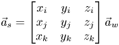
Consider a world coordinate system described with axes $[\vec {x}, \vec {y}, \vec {z}]$ and a ship coordinate system described with axes $[\vec {i}, \vec {j}, \vec {k}]$
 . Each axis from the world coordinate system may be expressed as a combination of axes from the ship coordinate system:

Thus, an arbitrary vector $\vec {a}$ described with three-dimensional coordinates $\vec {a}_w$
 in the world coordinate system transforms to the ship coordinate system as follows:
Let $\vec {s}$ be the origin of the ship coordinate system described in the world coordinate system:

Consider a point $P$ in the environment with coordinates $\vec {p}_w$
 in the world coordinate system and $\vec {p}_s$
 in the ship coordinate system. The transformation that relates the coordinates of $P$
 in each coordinate system can be defined as (Hartley and Zisserman, Reference Hartley and Zisserman2004)

Further, consider a camera coordinate system described with axes $[\vec {\chi }, \vec {\gamma }, \vec {\kappa }]$ . Axis $\vec {\chi }$
 is oriented from left to right, axis $\vec {\gamma }$
 is oriented downwards and axis $\vec {\kappa }$
 is forward oriented. Let each axis from the ship coordinate system be expressed as a combination of axes from the camera coordinate system:

Let $\vec {c}$ be the origin of the camera coordinate system described in the ship coordinate system:

The transformation relating coordinates of a point $P$ described in the ship coordinate system or in the camera coordinate system may be similarly determined:


Thus, for a point described with coordinates $\vec {p}_w$ in the world coordinate system, the corresponding coordinates $\vec {p}_c$
 in the camera coordinate system can be computed with two sequential transformations. Once a point is described in the camera coordinate system, it is possible to use camera models for its projection as a virtual point in the image scene.
Let $p = [\chi \ \gamma \ \kappa ]^\textrm {T}$ be a scene point described in the camera coordinate system and let $i = [u \ v]^\textrm {T}$
 be its corresponding image projection in pixels. Ideally, the relationship between $p$
 and $i$
 may be expressed with the pinhole model, which is given by (Hartley and Zisserman, Reference Hartley and Zisserman2004)

Parameters $[f \Delta _u^{-1}\ \ f \Delta _v^{-1} \ \ c_u \ \ c_v]$ are called intrinsic parameters or simply camera parameters. This model assumes a process of central projection. Light from the scene reaches the camera through a unique point referred to as the camera centre. Measurements are sampled in a plane at a distance $f$
 from the camera centre. Distance $f$
 is usually referred to as the focal distance of the camera. The rest of the camera parameters represents the conversion from sensor plane to pixel units. Note that more sophisticated models may be developed by taking into consideration mechanical properties of the lens and typical hardware components (Mahmoudi et al., Reference Mahmoudi, Sabzehparvar and Mortazavi2021).
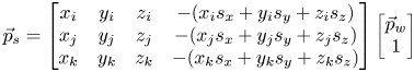
From the correspondences of image coordinates and three-dimensional positions, the camera parameters can be estimated by minimising the error between image observations and their respective model projections. Simplified procedures to estimate the camera parameters are usually based on the camera observation of structures with known dimensions and easily detectable features. A common procedure is based on the observation of a known planar pattern at a few different orientations (Zhang, Reference Zhang2000). Figure 2 shows examples of such calibration patterns as measured by a camera. These planar patterns may be printed with any commercial printer.
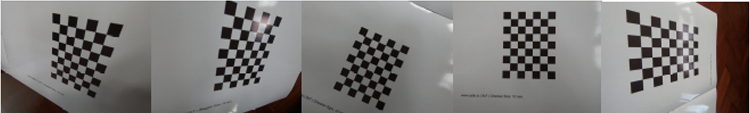
Figure 2. Observation of known planar patterns for calibration
The size of each square from the images above is known. Thus, it is possible to define three-dimensional coordinates for each square intersection of the pattern. Calibration parameters may be estimated from these correspondences with open source libraries. The present work uses the open source library OpenCV (Bradski, Reference Bradski2000) for most implementations regarding image manipulation. Particularly, the library is used for calibrating the camera, projection of points and synthesis of graphical elements. Figure 3 shows the projection of virtual points associated with the previous calibration pattern using the OpenCV library.
Figure 3. Detections and corresponding projections of the coplanar virtual points used in the calibration
Note that all virtual points drawn above belong to a particular plane $\pi$ coincident with the calibration pattern. An arbitrary plane $\pi$
 may be parametrised by a three-dimensional point $\pi _p$
 belonging to $\pi$
 along with two unitary orthogonal vectors $\pi _{\hat {n}_x}$
 and $\pi _{\hat {n}_y}$
 parallel to $\pi$
 . Thus, the coordinates of other points $p$
 from the plane may be computed from $\pi _p$
 and a linear combination of $\pi _{\hat {n}_x}$
 and $\pi _{\hat {n}_y}$
 :
:

A particular set of points of the plane $\pi$ may be defined by iterating different pairs $(\lambda _1,\lambda _2)$
 . Assuming that plane parameters $\pi _p$
 , $\pi _{\hat {n}_x}$
 and $\pi _{\hat {n}_y}$
 are described with respect to the camera coordinate system, auxiliary lines can be straightforwardly projected into the scene with above camera models.
2.3 Experimental setup
Consider a video generated from a navigation experiment by the TPN-USP Ship Maneuvering Simulation Center. The TPN-USP is the largest Brazilian ship manoeuvring simulation centre, equipped with three full-mission simulators and three tug stations, as well as one part-task simulator. Tannuri et al. (Reference Tannuri, Rateiro, Fucatu, Ferreira, Masetti and Nishimoto2014) describe the mathematical model adopted in the simulator, and Makiyama et al. (Reference Makiyama, Szilagyi, Pereira, Alves, Kodama, Taniguchi and Tannuri2020) presents the visualisation framework, able to generate realistic images of the maritime scenario, in real-time. In the video from the experiment, all geometrical parameters are accurately known. Figure 4 illustrates the scene measured by the camera alongside the geometry of the ship from the simulation.

Figure 4. Ship geometry and visualisation of the simulation experiment
An estimation of the intrinsic parameters of the camera is provided. A set of points with known coordinates may be projected into the image to validate accurateness or to further optimise camera parameters. This is illustrated in Figure 5.
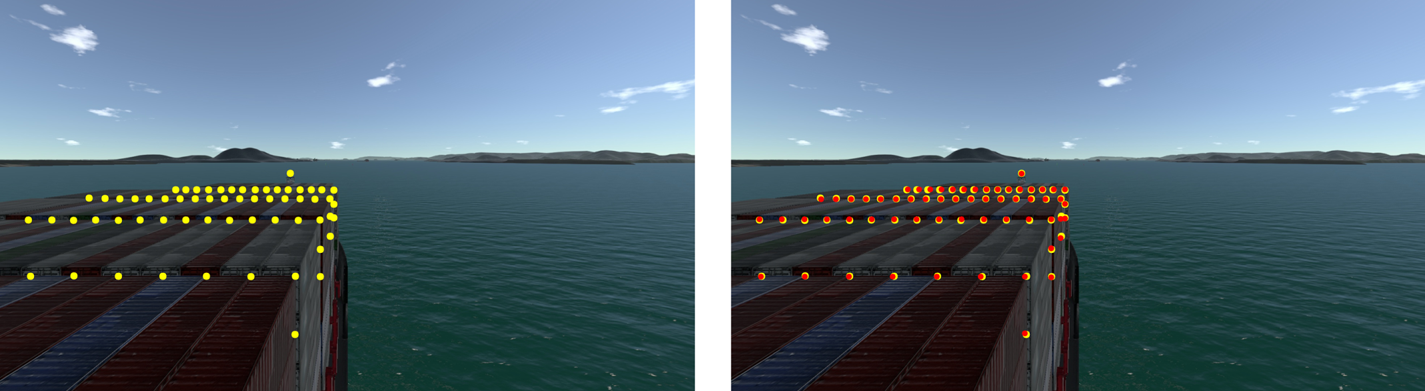
Figure 5. Detections in the image plane are highlighted on the left; projections from the ship geometry and the camera parameters are shown on the right
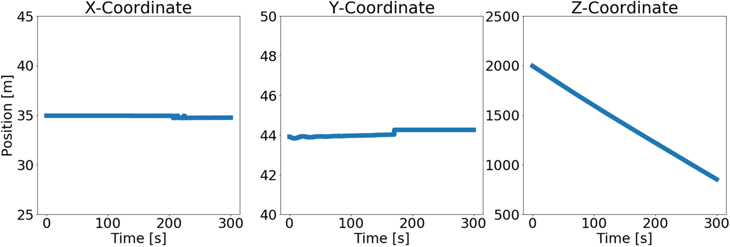
The state of the ship with respect to the world coordinate system is known from the simulation outputs. Figure 6 shows the ship position as a function of time.
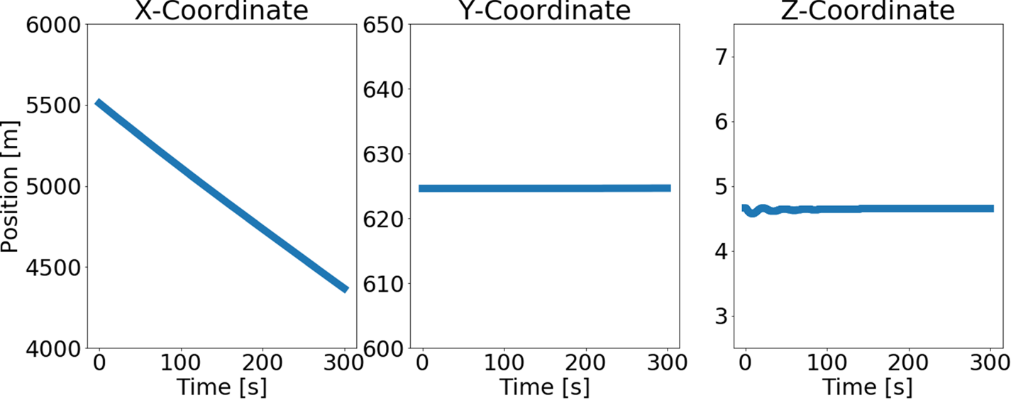
Figure 6. Ship position as a function of time with respect to the world coordinate system
Each buoy has fixed coordinates in the world coordinate system during the simulation. Thus, their instantaneous relative position in the ship coordinate system may be computed with expressions from Equations (2.4) and (2.5).
These coordinates in the ship coordinate system may be transformed to the camera coordinate system with expressions from Equations (2.8) and (2.9). Figure 7 shows the instantaneous relative position of one of the buoys with respect to the camera coordinate system.

Figure 7. Buoy position as a function of time with respect to the camera coordinate system
Further, consider another video from a real experiment of a ship navigating through a channel delimited by nautical buoys with a fixed onboard camera. Figure 8 summarises the installation of the camera for this experiment alongside relevant geometrical information from the ship. The ship orientation with respect to the world coordinate system is assumed to be constant and known during the entire experiment. Note that in this real experiment, the instantaneous position of nearby obstacles are unknown.
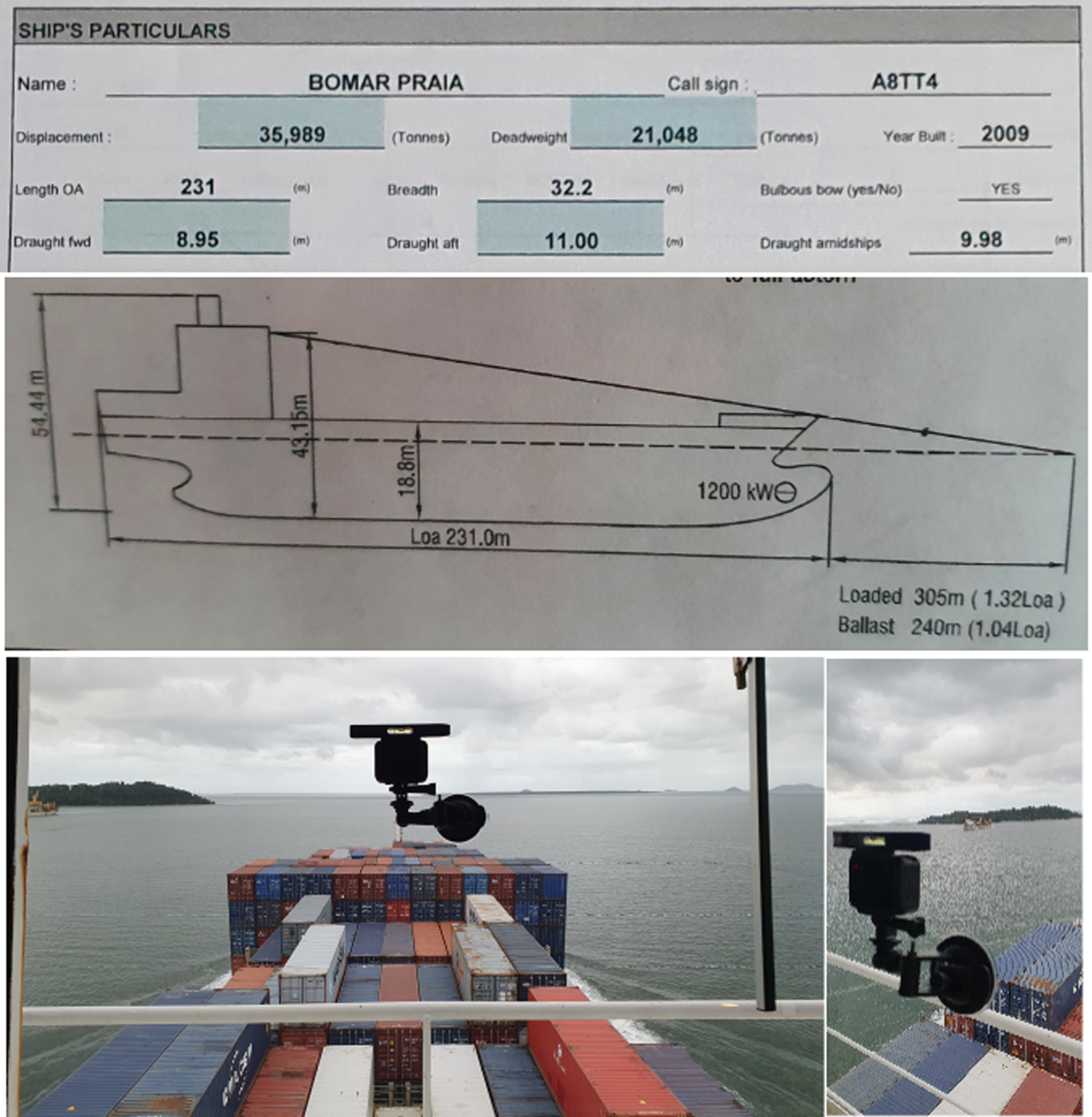
Figure 8. Geometrical information from the ship (top picture) and installation of the camera in the ship (bottom picture)
Intrinsic parameters of the camera are known from calibration procedures, such as the implementation from the OpenCV library described in the previous section. The camera position and orientation with respect to the ship frame must be known. Thus, it is interesting to install the camera in a known location from the ship such as in its bridge or its cabin. Then, these parameters may be estimated after installation with information from the ship geometry, which are typically available in the pilot cardboard and the wheelhouse poster, as shown in Figure 8.
If there are known correspondences between camera measurements and three-dimensional coordinates, it is possible to directly estimate the camera position and orientation after installation. For example, consider that all containers from the scene have known dimensions. For each block of adjacent containers, a set of correspondences may be defined with an arbitrary origin and adjacent container points. Then, optimising each set of correspondences yields estimates for the position and orientation for each block of containers. Finally, an estimation for the orientation of the camera may be defined assuming the alignment of all containers with the ship coordinate system. Figure 9 exemplifies the procedure with visible points from four blocks of adjacent containers.
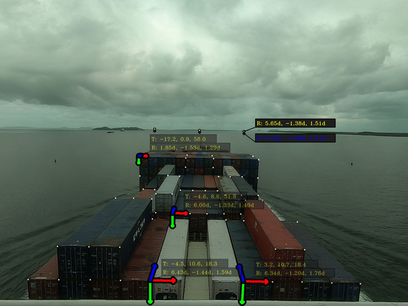
Figure 9. Camera calibration with visible points from onboard containers
Henceforth, the camera position and orientation is assumed to be known with respect to the ship coordinate system. Virtual points around the surface of the sea may be determined from Equation (2.11) by combining the ship draft with the installed camera position and orientation.
For a plane $\pi$ described with respect to a coordinate system external to the camera, the corresponding plane parameters $\pi _p$
 , $\pi _{\hat {n}_x}$
 and $\pi _{\hat {n}_y}$
 must be transformed to the camera coordinate system. Assuming knowledge of the rotation matrix relating both frames along with the origin of the external coordinate system, each vector $\pi _{\hat {n}_x}$
 and $\pi _{\hat {n}_y}$
 may be transformed to the camera coordinate system with a matrix multiplication, as presented in Equation 2.2. The point plane $\pi _p$
 may be transformed similarly as in Equations (2.4), (2.5), (2.8) and (2.9).
3. Results
This section proposes simple virtual information elements that may be rendered on the navigation scene of the previous experiment.
3.1 Simple highlighting
In the simulation experiment, as the position of each buoy in the camera coordinate system is known, it is possible to determine the corresponding projection coordinates in the camera scene by using Equation (2.10). These coordinates may be used for an automatic highlight of such obstacles. A simple form of a highlight is the synthesis of a rectangle as indicated in Figure 10. The obstacle coordinates with respect to the world, ship and camera frame is displayed next to the obstacle projection on the navigation scene.
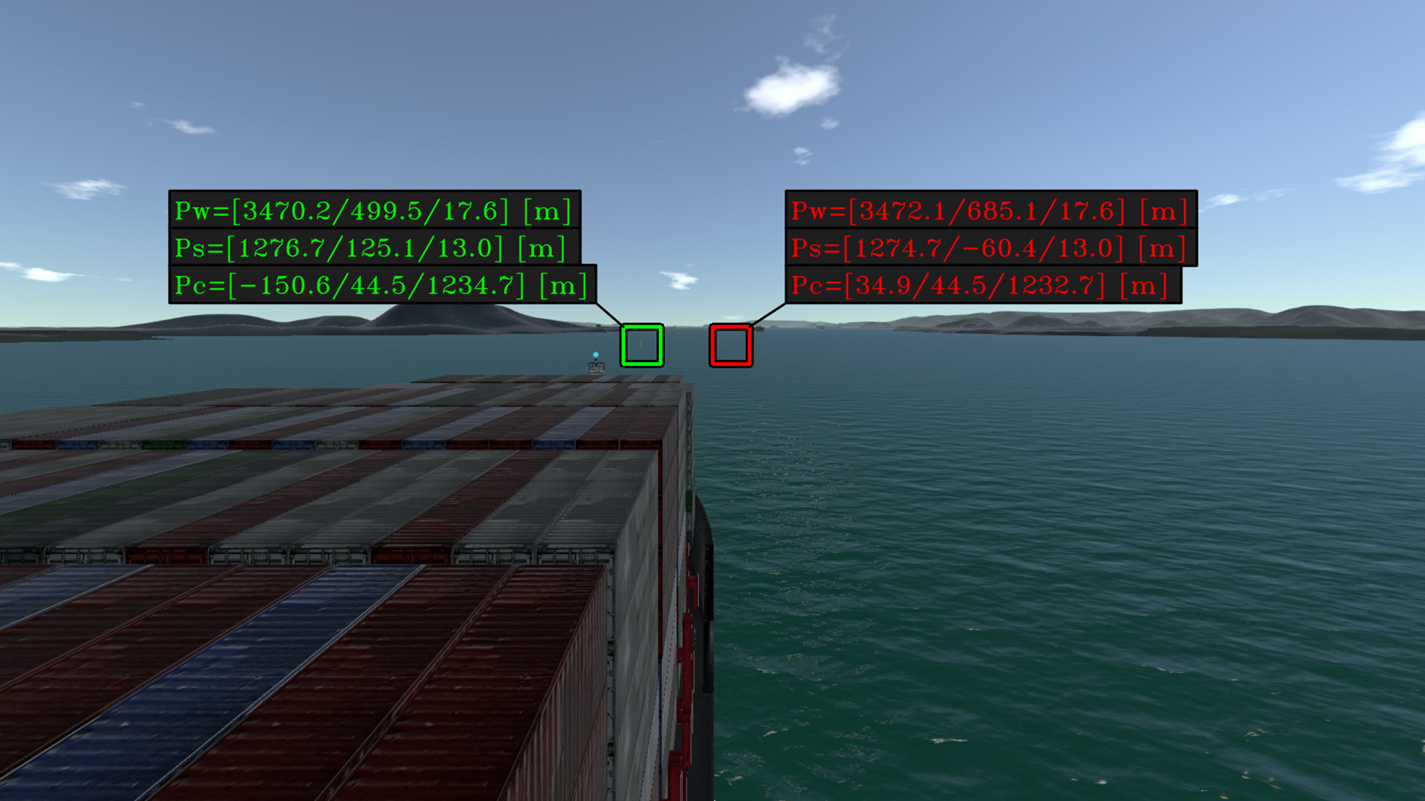
Figure 10. Simple highlighting for each buoy with a summary of coordinates expressed in different frames
3.2 Planar highlighting
Another form of highlight for a surrounding obstacle may be defined with the projection of a particular set of planar points around its position. Consider the set of points belonging to a plane $\pi$ according to Equation (2.11). The expression describes a plane $\pi$
 with a point $\pi _p$
 and two unitary vectors $\pi _{\hat {n}_x}$
 and $\pi _{\hat {n}_y}$
 :
:

Assume that unitary vectors $\pi _{\hat {n}_x}$ and $\pi _{\hat {n}_y}$
 are aligned with the surface of the sea. Thus, each pair $(\lambda _1, \lambda _2)$
 yields three-dimensional coordinates of a point near $\pi _p$
 at the surface of the sea. Different highlight visualisations may be determined depending on the set of $(\lambda _1, \lambda _2)$
 .
.
A rectangular highlight consists of two sets of parallel lines in which each line from one set is perpendicular to all lines from the other set. Such a highlight may be defined with the following expressions for pairs $(\lambda _1, \lambda _2)$ :
:

where $\Delta L_x$ and $\Delta L_y$
 define the distances between adjacent and parallel lines. The integer $i_x$
 iterates from $-N_x$
 to $N_x$
 and $i_y$
 iterates from $-N_y$
 to $N_y$
 . Adjacent points are connected with lines. Figure 11 shows a rectangular highlight computed with the following parameters:


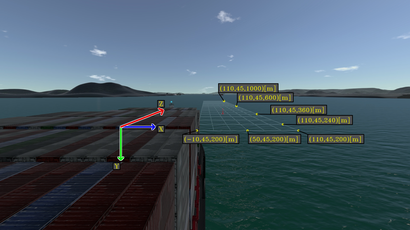
Figure 11. Auxiliary rectangular grid for points in the camera frame. Each rectangle of the grid has dimensions $40\ \textrm {m} \times 20\ \textrm {m}$
Alternatively, a circular highlight consists of sets of co-planar circles around a given point $\pi _p$ . Each point from each circle may be described by an angle $\theta$
 with respect to the plane vector $\pi _{\hat {n}_x}$
 and by a radius $r_i$
 with respect to the plane point $\pi _p$
 . Such a highlight may be defined by the following expressions for pairs $(\lambda _1, \lambda _2)$
 :
:

where $R_{r}$ is a list with different radius to be displayed, $\max (R_{r})$
 represents the element of maximum value in $R_{r}$
 and $r_i$
 denotes an element of $R_r$
 that is being iterated. Pairs $(\lambda _1, \lambda _2)$
 generated by the variation of $\theta$
 with a fixed $r_i$
 yields circles with radius $r_i$
 . These circles may be divided into sections by the computation of $(\lambda _1, \lambda _2)$
 with a fixed $\theta$
 and variable $r_i$
 . Here $\Theta _{r}$
 is a list with different $\theta$
 for sectioning such circles. Figure 12 shows a circular highlight computed with the following parameters:


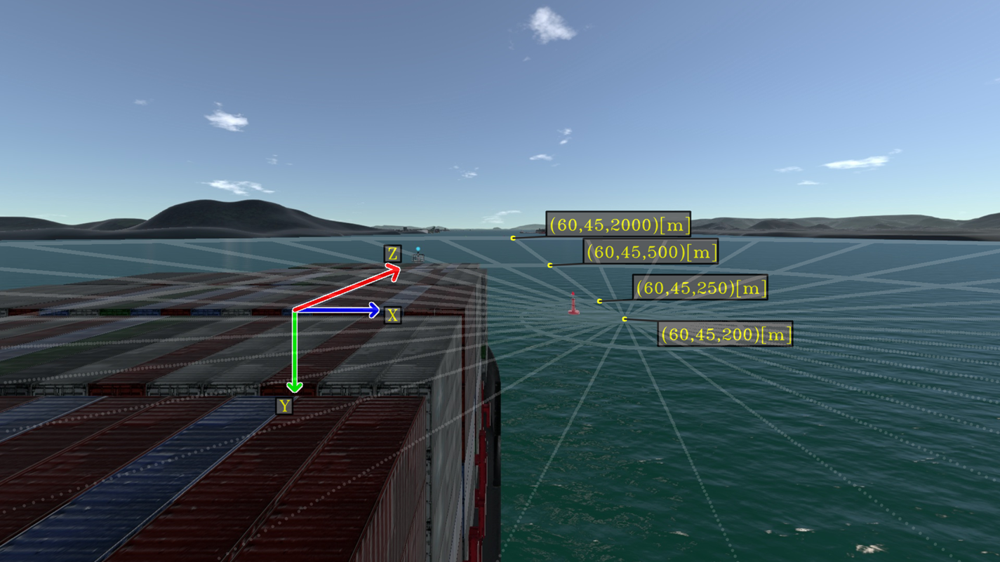
Figure 12. Auxiliary cylindrical grid for points in the camera frame. Each circle is divided into 32 sections
If there are external systems providing information about surrounding obstacles at sea, such as their relative position with respect to the ship, their projection in the camera scene may be automatically enhanced by virtual elements to assist in their identification. This situation is exemplified by the video from the experiment of the ship manoeuvring simulator. Generally, for a real implementation of such an automatic highlight, it is necessary to integrate the system with typical onboard equipment from the ship. In the video from the real experiment, where no prior information about surrounding obstacles is available, image-processing techniques may be also applied to determine the projection of each obstacle in the navigation scene.
Furthermore, note that the aforementioned auxiliary lines defined by Equations (2.11), (3.1) and (3.4) may be used to assist in the spatial perception of the scene. A potentially useful application would be to highlight the expected route in the navigation scene to assist in its perception by operators. Instead of rendering a planar highlight around the coordinates of a given obstacle, a planar highlight around points from the expected trajectory may assist in the perception of the ship route.
4. Discussion
In this section, potential applications of navigational assistance in restricted waters are discussed in terms of the proposed visual elements.
4.1 Route highlighting
In the previous simulation, the ship is navigating in a straight line with known velocity. In such situations, a rectangular highlight in front of the ship corresponds to the expected trajectory of the ship. Figure 13 exemplifies the implementation in the previous simulation experiment with a rectangular highlight delimiting the expected trajectory of the ship.

Figure 13. Rectangular highlight showing the expected trajectory for the ship in the simulation
A similar rectangular highlight may be drawn on top of the video from the real experiment as the ship navigates with approximately constant velocity in a straight line. Figure 14 illustrates this implementation.
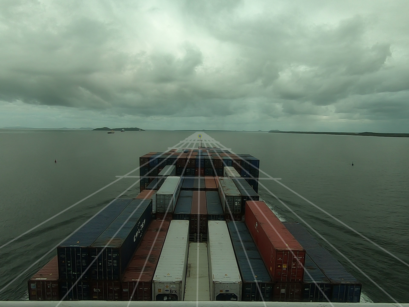
Figure 14. Rectangular highlight showing expected trajectory for the ship in reality
Another useful representation for the expected trajectory of the ship is in the form of waypoints. Each waypoint may be projected into the image scene with a circular highlight. As the ship is travelling with constant velocity, its trajectory may be represented by colinear waypoints. Figure 15 illustrates the visualisation with two waypoints in front of the ship.

Figure 15. Circular highlight representing waypoints of the expected trajectory for the ship in the simulation
Figure 16 illustrates a similar implementation in the recorded video from the aforementioned real experiment.

Figure 16. Circular highlight representing waypoints of the expected trajectory for the ship in reality
4.2 Obstacle highlighting
Let each buoy of the previous simulation be an obstacle to be highlighted in the image scene with a simple highlight. Assume that information about surrounding obstacles is available and consider an additional onboard system that is able to provide information about nearby obstacles in the form of different attributes. For example, attributes such as identification, name, type, status, position with respect to map and position with respect to ship. Further, assume that the corresponding obstacle attributes are automatically rendered into a graphical summary. Such a graphical summary may be overlaid next to the obstacle projection in the navigation scene, as shown in Figure 17.

Figure 17. Information highlight for each buoy in the simulation
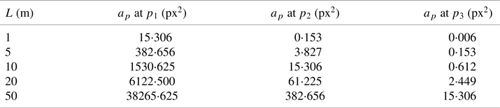
Note that points that are very far from the ship have a corresponding small projection in the image scene. It is interesting to estimate the maximum distance in which an obstacle is still observable by the camera. A simplified analysis may be carried out as follows. Consider a pinhole model expressed by the set of intrinsic parameters $[f_u, f_v, c_u, c_v]$ . Further, assume that the obstacle is represented as a simple planar square object with size $L$
 positioned at a point $p$
 . Each vertex $p^{li}$
 of this square may be projected into the image scene:

The projection area $a_p$ in pixel$^2$
 may be computed as a function of the projection of each vertex of the square:

Visible objects should have a projection area $a_p$ bigger than $1$
 pixel$^2$
 . Table 1 presents $a_p$
 as a function of different $L$
 at points $p_1 =[50,15,200]$
 , $p_2=[50,15,2{,}000]$
 and $p_3=[50,15,10{,}000]$
 for intrinsic camera parameters $[f_u, f_v, c_u, c_v]=[790, 770, 960, 440]$
 .
.
Table 1. Calculated $a_p$ at $p^W_i$
 for different values of $L$

Thus, for example, a square with an area of 1 m$^2$ would not be visible at a distance of 2,000 m but would be detectable at a distance of 200 m from the camera. Still, if $a_p$
 is not sufficiently greater than 1 px$^2$
 , its projection in the image scene may be very difficult to acknowledge. In such scenarios, the scene could be zoomed-in around the obstacle projection to assist in their identification. The open source library OpenCV (Bradski, Reference Bradski2000) provides zoom-in operations that may be used for rendering such amplifications of far obstacles. These amplified windows may be automatically displayed next to each obstacle projection as illustrated in Figure 18.

Figure 18. Amplified windows of surrounding obstacle projections in the simulation
Figure 19 shows two amplified windows for each buoy of the aforementioned real experiment. Different from the simulation experiment, the relative position of these buoys with respect to the ship and the camera are not known. In such cases, each zoom window needs to be manually initialised by an operator. Note that image processing methods may be performed for further automatic tracking of each initialised region.
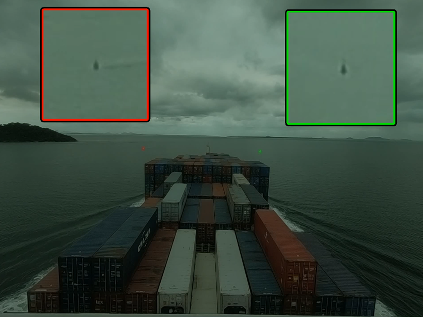
Figure 19. Amplified windows of surrounding obstacle projections in reality
4.3 Spatial perception
In cases where external information about surrounding obstacles is not available, it is possible to estimate the relative position of visible obstacles in the image scene with planar highlights. Figure 20 shows a rectangular highlight with points described in the ship coordinate system. An estimation for the relative position of the buoy may be inferred by the intersection of the buoy projection in the image scene with each auxiliary line of the rectangular grid.

Figure 20. Auxiliary rectangular grid for estimating the relative position of surrounding obstacles in the simulation. Each rectangle of the grid has dimensions $100\ \textrm {m} \times 25\ \textrm {m}$
Figure 21 shows a rectangular highlight in the real experiments with a grid of dimensions $100\,{\rm m} \times 25\,{\rm m}$ .
.
Figure 21. Auxiliary rectangular grid for estimating the relative position of surrounding obstacles in reality. Each rectangle of the grid has dimensions $100\ \textrm {m} \times 25\ \textrm {m}$
Note that the right buoy intersects the rectangular grid at the sixth parallel line of the grid, which represents an approximate lateral distance of $25 \times 6 = 150$ m. Correspondingly, the left buoy intersects the rectangular grid at the fifth parallel line of the grid, which yields an approximate lateral distance of $25 \times 5 = 125$
 m. Combining both results yields estimates of 275 m for the distance between both buoys. Accordingly, the theoretical distance between them is approximately 280 m when both buoys are in their map position.
Another useful representation for estimating the relative position of the buoy may be displayed with a circular highlight. Figure 22 shows a circular highlight with points described in the ship coordinate system.
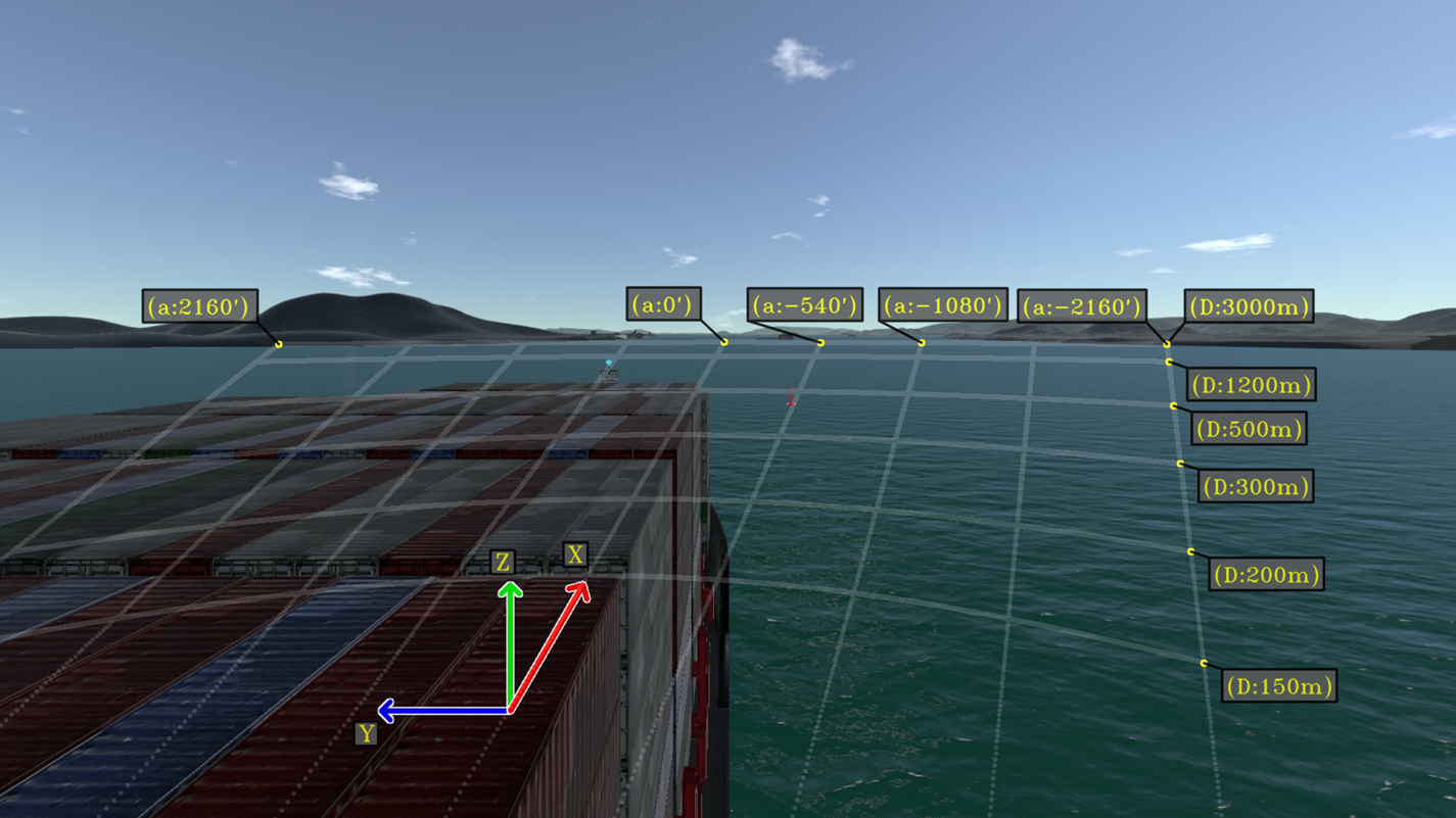
Figure 22. Auxiliary lines described with respect to the ship frame. Lines are drawn ranging from $\theta _{\textrm {min}} = -36^{\circ } = -2{,}160'$ to $\theta _{\textrm {max}} = 36^{\circ } = 2,160'$
Similarly, an estimation for the buoy relative position may be determined from the intersection of its projection with each auxiliary line. From the augmented scene of the above example, it is possible to estimate that the buoy is at an approximate distance of 500 m from the ship with an angle of $-9^\circ$ with respect to the ship $x$
 -axis.
Note that the augmented scenes from this section are designed considering a scenario of a ship travelling in restricted waters with fixed obstacles. In such scenarios, to prevent collisions, it is important that operators acknowledge the relative position of surrounding obstacles along the expected trajectory of the ship. As the proposed enhanced scenes from this section assist in the perception of these important elements, these scenes may be combined into a navigational assistance equipment based on augmented reality.
Alternative enhanced scenes may be adapted from the current work towards other navigation scenarios. As the development of optimal visualisations combining pertinent virtual elements depends on the particular operation of the user, further research is suggested to cover other types of standardised navigation operations.
5. Conclusion
Foundations regarding augmented reality methods were discussed throughout the paper. Examples of enhanced scenes for a monitor AR solution were proposed in the context of a ship navigating with constant velocity in restricted waters. As each augmented scene assist in the perception of the navigation environment, these visualisations are potentially helpful for the corresponding ship operators. However, to adequately embed these augmented scenes into helpful equipment, designed visualisations shall be further validated considering usability requirements from typical operations.
The development of an operational augmented reality system for navigational assistance is still a complex task. For a real implementation, the ship state with respect to the world coordinate system needs to be accurately determined along with the camera parameters. To ensure a proper alignment between real and virtual marks, information regarding the truth position of nearby obstacles and ship surroundings needs to be accurately determined by onboard ship systems. Additionally, the integration of such different equipment needs to robustly address real-time constraints which may be inherently complex.
Despite the challenges, the development of equipment with augmented reality methods is further suggested as it has the potential to significantly contribute to the overall efficiency and safety of maritime operations. It should be noted that although further research with real implementations may be extremely expensive owing to the requirement of high-precision sensors, usability research may be appropriately performed with any full-mission ship manoeuvring simulator as presented in the present work. Therefore, as a general recommendation, the authors suggest that user interface research for MAR systems should be preliminary performed with a ship manoeuvring simulator. In such simulations, all geometrical parameters are known, which facilitates the development of ideal visualisations without the need of extremely accurate equipment.
Acknowledgements
The authors thank Petrobras and Brazilian National Agency for Petroleum, Natural Gas and Biofuels (ANP) for supporting this research project. B.G.L. thanks the Coordination for the Improvement of Higher Education Personnel (CAPES) for the scholarship. E.A.T. thanks the CNPq – Brazilian National Council for Scientific and Technological Development for the research grant (process 310127/2020-3).