


1. INTRODUCTION
Code phase Global Navigation Satellite System (GNSS) receivers convert the measured satellite pseudoranges into estimates of the position and clock offset of the receiver. The typical implementation of the solution algorithm is an iterative, linearized least squares method. Assuming that pseudoranges from m non-coplanar satellites are measured, the direction cosines matrix
 ${\bf{G}}$
is formed and used to solve an overdetermined set of equations. Since the pseudoranges themselves are noisy, the resulting estimates of position and time are random variables. To describe the accuracy of this solution, it is common to describe it statistically via the error covariance matrix, equal to the inverse of
${\bf{G}}$
is formed and used to solve an overdetermined set of equations. Since the pseudoranges themselves are noisy, the resulting estimates of position and time are random variables. To describe the accuracy of this solution, it is common to describe it statistically via the error covariance matrix, equal to the inverse of
 ${\bf{G}}^{T}{\bf{G}}$
scaled by the User Range Error (URE) (Misra and Enge, Reference Misra and Enge2006). Rather than considering the individual elements of this covariance matrix, users frequently reduce it to a scalar performance indicator. The most common of these is the Geometric Dilution of Precision (GDOP), the square root of the trace of
${\bf{G}}^{T}{\bf{G}}$
scaled by the User Range Error (URE) (Misra and Enge, Reference Misra and Enge2006). Rather than considering the individual elements of this covariance matrix, users frequently reduce it to a scalar performance indicator. The most common of these is the Geometric Dilution of Precision (GDOP), the square root of the trace of
 $\lpar {\bf{G}}^{T}{\bf{G}} \rpar ^{-1}$
; equivalently, this is the square root of the sum of the variances of the estimates without the URE scaling. Other possible measures of performance are the Position (PDOP), Horizontal (HDOP), Vertical (VDOP), and Time (TDOP) portions of GDOP. One could also include the off-diagonal elements of the covariance matrix such as are used for the circular error probability (Conley et al., Reference Conley, Cosentino, Hegarty, Kaplan, Leva, Uijt de Haag and Van Dyke2006); when non-zero, these off-diagonal terms describe any directional characteristic in the error ellipsoid which is lost by focusing only on the PDOP.
$\lpar {\bf{G}}^{T}{\bf{G}} \rpar ^{-1}$
; equivalently, this is the square root of the sum of the variances of the estimates without the URE scaling. Other possible measures of performance are the Position (PDOP), Horizontal (HDOP), Vertical (VDOP), and Time (TDOP) portions of GDOP. One could also include the off-diagonal elements of the covariance matrix such as are used for the circular error probability (Conley et al., Reference Conley, Cosentino, Hegarty, Kaplan, Leva, Uijt de Haag and Van Dyke2006); when non-zero, these off-diagonal terms describe any directional characteristic in the error ellipsoid which is lost by focusing only on the PDOP.
It is known that the GDOP is a function of the satellite geometry; with only a few visible satellites in poor locations the GDOP can become quite large. However, for a future with multiple, fully occupied GNSS constellations it is expected that receivers would select those satellites to track so as to achieve the best possible performance; see, for example, Gerbeth et al. (Reference Gerbeth, Felux, Circiu and Caamano2016) and Walter et al. (Reference Walter, Blanch and Kropp2016). Hence, we think that an understanding of both how small the GDOP and PDOP can be as a function of the number of satellites visible and the characteristics of the constellations that meet those bounds are of value in the satellite selection process. It should be possible to exploit those characteristics (for example, selecting satellites at the right ratio of high and low elevation and with azimuths that satisfy balance, described below) in selecting a subset of satellites (Swaszek et al., Reference Swaszek, Hartnett and Seals2016).
Investigating the best possible GNSS satellite constellation with respect to GDOP is not a new problem. The case of m=4 satellites, with reference to optimising the tetrahedron formed by their locations, has been considered by multiple authors, see for example Kihara and Okada (Reference Kihara and Okada1984). The best constellations of four, five and six satellites are described in Spilker (Reference Spilker1996); the case of five satellites from two GNSS constellations is considered in Teng et al. (Reference Teng, Wang and Huang2016). A general lower bound for m satellites from one constellation is known,
 $\hbox{GDOP}\ge \sqrt {10\over m}$
, but does not restrict the satellites’ elevations to be above the horizon (Zhang and Zhang, Reference Zhang and Zhang2009).
$\hbox{GDOP}\ge \sqrt {10\over m}$
, but does not restrict the satellites’ elevations to be above the horizon (Zhang and Zhang, Reference Zhang and Zhang2009).
The goal of this paper is to provide tight lower bounds to the GDOP and PDOP for the case of m≥4 non-coplanar satellites when the satellites must be at or above the horizon. Specifically, for a single constellation these bounds are
 $$\hbox{GDOP}\ge \sqrt {11{\cdot}89\over m}\quad \hbox{and}\quad\hbox{PDOP}\ge \sqrt {10{\cdot}47 \over m}$$
The following sections develop these bounds, examine their achievability, modify them to allow for a non-zero mask angle, and then extend them to satellites from L non-synchronised satellite constellations. Details of the less elucidating proofs are relegated to Appendices to improve readability.
2. BOUNDING GDOP
The direction cosines matrix for m satellites from a single constellation in three dimensions using an East, North, and Up coordinate frame is
 $${\bf{G}}=\left[\matrix{ e_{1} & n_{1} & & u_{1} & 1 \cr e_{2} & n_{2} & & u_{2} & 1 \cr && \vdots && \cr e_{m} & n_{m} & & u_{m} & 1}\right]$$
in which
 $(e_{k},n_{k},u_{k})$
is the unit vector pointing toward the k
th
satellite from the receiver's location. The GDOP is defined as
$(e_{k},n_{k},u_{k})$
is the unit vector pointing toward the k
th
satellite from the receiver's location. The GDOP is defined as
 $$\hbox{GDOP}=\sqrt{\hbox{trace}\lcub \lpar {\bf{G}}^{T}{\bf{G}} \rpar^{-1} \rcub }$$
and combines terms proportional to the East, North, Up, and time errors in the GNSS solution; the PDOP ignores the time portion.
For convenience consider the square of the GDOP
 $${\hbox{GDOP}}^{2}=\hbox{trace}\lcub \lpar {\bf{G}}^{T}{\bf{G}} \rpar^{-1} \rcub $$
The matrix
 ${\bf{G}}^{T}{\bf{G}}$
can be written in block partitioned form as
${\bf{G}}^{T}{\bf{G}}$
can be written in block partitioned form as
 $${\bf{G}}^{T}{\bf{G}}=\left[\matrix{{\bf{A}} & {\bf{B}} \cr {\bf{B}}^{T} & {\bf{C}}}\right]$$
with
 $$\eqalign{&{\bf{A}}=\left[\matrix{\displaystyle\sum_{k=1}^m e_{k}^{2} & \displaystyle\sum_{k=1}^m {e_{k}n_{k}} \cr \displaystyle\sum_{k=1}^m {e_{k}n_{k}} & \displaystyle\sum_{k=1}^m n_{k}^{2} }\right], \,\, \bf{B}=\left[ \matrix{ \displaystyle\sum_{k=1}^m {e_{k}u_{k}} & \displaystyle\sum_{k=1}^m e_{k} \cr \displaystyle\sum_{k=1}^m {n_{k}u_{k}} & \displaystyle\sum_{k=1}^m n_{k} }\right], \,\, and \cr & \bf{C}=\left[\matrix{ \displaystyle\sum_{k=1}^m u_{k}^{2} & \displaystyle\sum_{k=1}^m u_{k} \cr \displaystyle\sum_{k=1}^m u_{k} & m } \right]}$$
By construction both
 ${\bf{A}}$
and
${\bf{A}}$
and
 ${\bf{C}}$
are symmetric. Assuming at least four non-coplanar satellites, then
${\bf{C}}$
are symmetric. Assuming at least four non-coplanar satellites, then
 ${\bf{G}}$
is full rank and
${\bf{G}}$
is full rank and
 ${\bf{G}}^{T}{\bf{G}}$
is positive definite. Being principal submatrices of
${\bf{G}}^{T}{\bf{G}}$
is positive definite. Being principal submatrices of
 ${\bf{G}}^{T}{\bf{G}}$
then both
${\bf{G}}^{T}{\bf{G}}$
then both
 ${\bf{A}}$
and
${\bf{A}}$
and
 ${\bf{C}}$
are also positive definite and invertible (Horn and Johnson, Reference Horn and Johnson2013).
${\bf{C}}$
are also positive definite and invertible (Horn and Johnson, Reference Horn and Johnson2013).
Inverting
 ${\bf{G}}^{T}{\bf{G}}$
yields
${\bf{G}}^{T}{\bf{G}}$
yields
 $${\hbox{GDOP}}^{2}= \hbox{trace}\lcub \lpar {\bf{A}}-{\bf{B}}{\bf{C}}^{{-1}}{\bf{B}}^{T} \rpar^{-1} \rcub +\hbox{trace}\lcub \lpar {\bf{C}}-{\bf{B}}^{T}{\bf{A}}^{{-1}}{\bf{B}} \rpar^{-1} \rcub $$
which can be lower bounded
 $${\hbox{GDOP}}^{2}\ge \hbox{trace}\lcub {\bf{A}}^{-1} \rcub +\hbox{trace}\lcub {\bf{C}}^{-1} \rcub $$
with equality if and only if
 ${\bf{B}}$
is a zero matrix (Han et al., Reference Han, Chen, Gui, Li and Wei2013; Reference Han, Gui, Li and Du2014). Equivalently, to achieve minimum GDOP the satellite constellation should satisfy a set of “balance” conditions in the satellites’ locations
${\bf{B}}$
is a zero matrix (Han et al., Reference Han, Chen, Gui, Li and Wei2013; Reference Han, Gui, Li and Du2014). Equivalently, to achieve minimum GDOP the satellite constellation should satisfy a set of “balance” conditions in the satellites’ locations
 $$\sum_{k=1}^m e_{k} =0,\quad \sum_{k=1}^m n_{k} =0,\quad \sum_{k=1}^m {e_{k}u_{k}} =0,\quad\hbox{and}\quad \sum_{k=1}^m {n_{k}u_{k}} =0$$
Consider minimising the first term in Equation (8),
 $\hbox{trace}\lcub {\bf{A}}^{-1} \rcub $
. Simplifying notation, write
$\hbox{trace}\lcub {\bf{A}}^{-1} \rcub $
. Simplifying notation, write
 $${\bf{A}}=\left[\matrix{a & b\cr b & c} \right]$$
with elements defined in Equation (6). These elements must meet the constraints
 $$a+c=m-\sum_{k=1}^m u_{k}^{2}$$
(due to the e
k
and n
k
coming from the m satellites’ unit vectors) and b
2<ac (since
 ${\bf{A}}$
is positive definite); then
${\bf{A}}$
is positive definite); then
 $$\hbox{trace}\lcub {\bf{A}}^{-1} \rcub ={a+c\over ac-b^{2}}$$
A simple calculus argument yields that the minimum of this fraction occurs when b=0 and when a and c are both equal
 $$a=c={m-\sum_{k=1}^m u_{k}^{2}\over 2}$$
These results add two further conditions to the definition of constellation balance in Equation (9):
 $$\sum_{k=1}^m {e_{k}n_{k}} =0 \quad \hbox{and}\quad \sum_{k=1}^m e_{k}^{2} =\sum_{k=1}^m n_{k}^{2}$$
The result of the trace is
 $$\hbox{trace}\lcub {\bf{A}}^{-1} \rcub \ge {4\over m-\sum_{k=1}^m u_{k}^{2}}$$
Next, consider the second term in Equation (8),
 $\hbox{trace}\lcub {\bf{C}}^{-1} \rcub $
. Simplifying notation, write
$\hbox{trace}\lcub {\bf{C}}^{-1} \rcub $
. Simplifying notation, write
 $${\bf{C}}=\left[ \matrix{d & f \cr f & m} \right]$$
with elements defined in Equation (6). Assuming that all of the satellites are at or above the horizon, 0≤u
k
≤1 for all k, leads to the constraint 0≤d≤m. Since
 $u_{k}\ge u_{k}^{2}$
for each k, then f≥d. Finally, for
$u_{k}\ge u_{k}^{2}$
for each k, then f≥d. Finally, for
 ${\bf{C}}$
to be positive definite d>0 and\ f
2<dm. The
${\bf{C}}$
to be positive definite d>0 and\ f
2<dm. The
 ${\hbox{GDOP}}^{2}$
term is
${\hbox{GDOP}}^{2}$
term is
 $$\hbox{trace}\lcub {\bf{C}}^{-1} \rcub ={m+d\over dm-f^{2}}$$
Clearly f 2 should be as small as possible to minimise the trace, so f=d and
 $$\hbox{trace}\lcub {\bf{C}}^{-1} \rcub \ge {m+d\over d\lpar m-d \rpar }$$
Combining the results of Equations (12) and (18)
 $${\hbox{GDOP}}^{2}\ge {4\over m-d}+{m+d\over d\lpar m-d \rpar }={m+5d\over d\lpar m-d \rpar }$$
At this point one could follow two routes: (1) imagine that d (
 ${=}\sum_{k=1}^{n} u_{k}^{2}$
) can actually achieve any of the values in its range, 0<d<m, and find its best value to minimise the GDOP2 or (2) identify those values of d consistent with the balance constraints and optimise over that subset. The first method is considered here, leaving the second for discussion below. Taking a d derivative and equating it to zero yields the unique solution
${=}\sum_{k=1}^{n} u_{k}^{2}$
) can actually achieve any of the values in its range, 0<d<m, and find its best value to minimise the GDOP2 or (2) identify those values of d consistent with the balance constraints and optimise over that subset. The first method is considered here, leaving the second for discussion below. Taking a d derivative and equating it to zero yields the unique solution
 $$d^{\ast}={\left( \sqrt 6 -1 \right)m\over 5}\approx 0{\cdot}29 m$$
so
 $${\hbox{GDOP}}^{2}\ge {2\sqrt 6 +7\over m}\approx {11{\cdot}89\over m}$$
proving the first result.
3. ACHIEVABILITY
It has been suggested that constellations consisting of p satellites directly overhead (at zenith) and m−p satellites evenly spaced in azimuth at the horizon, for some integer p, have small GDOP (Zhang and Zhang, Reference Zhang and Zhang2009):
 $$\eqalign{& e_{k}=\left\{\matrix{\sin {2\pi k\over m-p}; & k=1,2,\ldots m-p \hfill \cr 0; \quad \quad \quad & k=m-p+1,\ldots m }\right. \cr & n_{k}=\left\{\matrix{\cos {2\pi k\over m-p}; & k=1,2,\ldots m-p \hfill \cr 0; \quad \quad \quad & k=m-p+1,\ldots m}\right. \cr & u_{k}=\left\{\matrix{0;& k=1,2,\ldots m-p \hfill \cr 1;& k=m-p+1,\ldots m}\right.}$$
(One can, of course, add an arbitrary rotation in azimuth to these unit vectors.) Clearly such a constellationFootnote
1
meets the balance conditions in Equations (9) and (14) as long as m−p≥3 (hint – use Lagrange's trigonometric identities). This results in d=p so that such a constellation has
 ${\hbox{GDOP}}^{2}$
exactly matching Equation (19) if one identifies p with d. Further, the optimisation over p exactly follows that for d above with the result that a constellation with 0·29 m satellites overhead and 0·71 m evenly spaced about the horizon would achieve
${\hbox{GDOP}}^{2}$
exactly matching Equation (19) if one identifies p with d. Further, the optimisation over p exactly follows that for d above with the result that a constellation with 0·29 m satellites overhead and 0·71 m evenly spaced about the horizon would achieve
 $${\hbox{GDOP}}^{2}={11{\cdot}89\over m}$$
Now, of course, m−p=0·71 m might not be an integer greater than or equal to 3. An obvious approach, then, is to round p up and down to the two nearest integers, choosing the constellation with best GDOP. This approach yields the optimum integer choice for p since
 ${\hbox{GDOP}}^{2}$
is convex in p for the range 0<p<m (proof: the second derivative of
${\hbox{GDOP}}^{2}$
is convex in p for the range 0<p<m (proof: the second derivative of
 ${\hbox{GDOP}}^{2}$
with respect to p is positive for the relevant range of p). Define
${\hbox{GDOP}}^{2}$
with respect to p is positive for the relevant range of p). Define
 ${\hbox{GDOP}}^{2}(m)$
as the better of these two constellations
${\hbox{GDOP}}^{2}(m)$
as the better of these two constellations
 $${\hbox{GDOP}}^{2}(m)=\min \left\{ {m+5p\over p\lpar m-p \rpar }, {{m+5\lpar p+1 \rpar \over \lpar p+1 \rpar \lpar m-p-1 \rpar } }\right\}$$
with
 $p=\left\lfloor {\left( \sqrt 6 -1 \right)\over 5}m \right\rfloor $
and 0<p<m. Figure 1 compares the optimum results of the previous section to those of the best achievable constellation. The upper subplot shows the number of satellites at zenith, p, versus the total satellite count, m; the lower subplot compares the resulting GDOP. The observation is that the resulting GDOPs, actual and lower bound, are nearly identical; that the bound is essentially achievableFootnote
2
.
$p=\left\lfloor {\left( \sqrt 6 -1 \right)\over 5}m \right\rfloor $
and 0<p<m. Figure 1 compares the optimum results of the previous section to those of the best achievable constellation. The upper subplot shows the number of satellites at zenith, p, versus the total satellite count, m; the lower subplot compares the resulting GDOP. The observation is that the resulting GDOPs, actual and lower bound, are nearly identical; that the bound is essentially achievableFootnote
2
.

Figure 1. Comparison of optimum and achievable GDOP results for one constellation versus the total number of satellites, m: (top) number of satellites, p, at zenith; (bottom) the resulting GDOP.
As an example of the match between the bound and practice, satellite positions were collected for the GPS constellation over a 24-hour period; the number of satellites above the horizon ranged from nine to 14. Figure 2, left, shows the GDOP performance for the best subset of seven satellites from the constellation as compared to the m=7 bound. Figure 2, right, shows the sky view of the seven satellites at the time marked by the arrow; two satellites (approximately 29% of the seven) high in the sky and five satellites distributed somewhat evenly about the horizon.
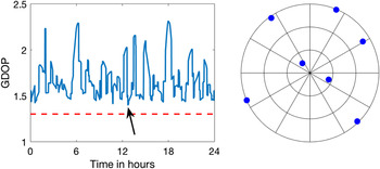
Figure 2. (left) Comparison of the lower bound (red, dashed) and actual (blue, solid) GDOP values for seven GPS satellites; (right) the constellation at the marked sample point.
4. POSITION DILUTION OF PRECISION (PDOP)
It might be more meaningful to discuss PDOP, ignoring the clock bias estimate's variance when describing performance. This is especially relevant below when discussing multiple constellations as GDOP, in that case, includes the variances of multiple additional clock biases.
Paralleling the analysis above for GDOP, partitioning
 ${\bf{G}}^{T}{\bf{G}}$
and computing its inverse (in partitioned form) yields
${\bf{G}}^{T}{\bf{G}}$
and computing its inverse (in partitioned form) yields
 $${\hbox{PDOP}}^{2}=\hbox{trace}\lcub \lpar {\bf{A}}-{\bf{B}}{\bf{C}}^{{-1}}{\bf{B}}^{T} \rpar^{-1} \rcub +\lpar {\bf{C}}-{\bf{B}}^{T}{\bf{A}}^{{-1}}{\bf{B}} \rpar ^{-1}_{[1,1]}$$
(the subscript [1, 1] on the second term indicating that only the top left element of this matrix is kept). Having
 ${\bf{B}}$
being the zero matrix minimises the first of these terms; it is shown in Appendix A that this also minimises the second. Using the notation of Equation (16)
${\bf{B}}$
being the zero matrix minimises the first of these terms; it is shown in Appendix A that this also minimises the second. Using the notation of Equation (16)
 $$\lpar {\bf{C}}-{\bf{B}}^{T}{\bf{A}}^{{-1}}{\bf{B}} \rpar ^{-1}_{[1,1]}\ge {m\over dm-f^{2}}$$
Further, setting f equal to its minimum value, d, yields the lower bound
 $${\hbox{PDOP}}^{2}\ge {4\over m-d}+{m\over d(m-d)}={m+4d\over d(m-d)}$$
which needs to be minimised over the choice of d. Taking a d derivative and equating it to zero yields the unique result
 $$d^{\ast}={\left( \sqrt 5 -1 \right)m\over 4}\approx 0{\cdot}31\,m$$
(slightly larger than that for minimum GDOP) and the second result
 $${\hbox{PDOP}}^{2}\ge {16\over \left( \sqrt 5 -1 \right)^{2}m}\approx {10{\cdot}47\over m}$$
achievable by a constellation with 31% of its satellites at zenith and the remaining 69% balanced at the horizon.
5. A NON-ZERO MASK ANGLE
The analyses above allowed for satellites on the horizon (and the optimum constellations put approximately 70% of the satellites there). What happens if a minimum elevation angle of ϕ is enforced? Note that the balance conditions on
 ${\bf{A}}$
and
${\bf{A}}$
and
 ${\bf{B}}$
only restrict the satellites’ azimuths. However, when working with
${\bf{B}}$
only restrict the satellites’ azimuths. However, when working with
 ${\bf{C}}^{-1}\,f$
can no longer equal its lower bound of d. For GDOP the goal is to minimise
${\bf{C}}^{-1}\,f$
can no longer equal its lower bound of d. For GDOP the goal is to minimise
 $$\hbox{trace}\lcub {\bf{C}}^{-1} \rcub ={m+d\over dm-f^{2}}$$
while for PDOP to minimise
 $${\bf{C}}^{-1}_{[1,1]}={m\over dm-f^{2}}$$
(the arguments of Appendix A hold independent of any mask angle) both of which are still achieved by making f as small as possible for the given d while satisfying the mask angle.
Let θ
k
,
 $\theta_{k}\ge \phi $
, represent the elevation angle of satellite k, then
$\theta_{k}\ge \phi $
, represent the elevation angle of satellite k, then
 $$d=\sum_{k=1}^m \sin^{2}\theta_{k}\quad\hbox{and}\quad f=\sum_{k=1}^m \sin \theta_{k}$$
Adding the requirement on d with a Lagrange multiplier, λ, it is equivalent to minimise
 $$F=\sum_{k=1}^m \sin \theta_{k} +\lambda \left( \sum_{k=1}^m \sin^{2}\theta_{k} -d \right)$$
over the θ k . Taking the θ k derivatives yields m necessary conditions
 $${\partial F\over \partial \theta_{k}}=\cos \theta_{k}\lpar 1+2\lambda \sin \theta_{k} \rpar =0$$
each of which has two solutions:
 $\theta_{k}=90^{\circ}$
(so that the cosine term is zero) or
$\theta_{k}=90^{\circ}$
(so that the cosine term is zero) or
 $$\theta_{k}=\cos^{-1}\left( -{1\over 2\lambda } \right)\equiv \theta$$
so that the second term is zero. Note that since 2λ is a constant, any elevation angles not equal to 90° are identical to each other. The solution, then, is that given a specific value for d there is some number, say p, of satellites at zenith and m−p at elevation angle θ so that p satisfies
 $$\sum_{k=1}^m u_{k}^{2} =p+\lpar m-p \rpar \sin^{2}\theta =d$$
The corresponding value for f is
 $$f=p+\lpar m-p \rpar \sin \theta =m-{m-d\over 1+\sin^{2}\theta}$$
Recall that the immediate goal is to make f as small as possible. Since m−d>0 this occurs when θ is as small as possible; hence, θ=ϕ. The resulting GDOP expression is
 $${\hbox{GDOP}}^{2}\ge {\beta\over m-p}+{m\gamma \over p(m-p)}$$
with notation
 $$\beta ={5-3\sin \phi -\sin^{2}\phi -\sin^{3}\phi \over \lpar 1-\sin \phi \rpar ^{2}\lpar 1+\sin \phi \rpar } \quad \hbox{and}\quad\gamma ={1+\sin \phi +\sin^{2}\phi +\sin^{3}\phi \over \lpar 1-\sin \phi \rpar ^{2}\lpar 1+\sin \phi \rpar }$$
This expression can be optimised to yield the best choice of p
 $$p^{\ast }={\sqrt {\gamma \lpar \gamma +\beta \rpar } -\gamma \over \beta }\ m$$
The lower bound, then, is the GDOP expression with this choice of p
 $${\hbox{GDOP}}^{2} \ge {\beta^{2} \over {\beta +2\gamma -2\sqrt {\gamma \lpar \gamma +\beta \rpar }}}\, {1\over m}$$
Figure 3 demonstrates these results (the solid curves) versus mask angle ϕ. The top subfigure shows the percentage of satellites at zenith, starting at 29% when ϕ=0 and increasing toward 50% as the mask angle increases. The lower subfigure shows the numerator of the
 ${\hbox{GDOP}}^{2}$
expression, equivalently
${\hbox{GDOP}}^{2}$
expression, equivalently
 ${m\times \hbox{GDOP}}^{2}$
, starting at 11·89 when ϕ=0 and increasing as ϕ increases. Note that this numerator grows slowly for small mask angles (i.e. a mask angle of 10° only increases the lower bound on GDOP by 12·6%), picking up speed for larger mask angles.
${m\times \hbox{GDOP}}^{2}$
, starting at 11·89 when ϕ=0 and increasing as ϕ increases. Note that this numerator grows slowly for small mask angles (i.e. a mask angle of 10° only increases the lower bound on GDOP by 12·6%), picking up speed for larger mask angles.

Figure 3. Results versus mask angle, ϕ: (top) the fraction of satellites at zenith; (bottom) the numerator of the DOP2 expression.
These results for PDOP are similar. With p satellites at zenith and m−p at elevation ϕ the resulting bound is
 $${\hbox{PDOP}}^{2}\ge {\mu \over m-p}+{m\nu \over p(m-p)}$$
with
 $$\mu ={4\over 1-\sin \phi }\quad\hbox{and}\quad\nu ={1\over \lpar 1-\sin \phi \rpar ^{2}}$$
The optimum choice for p is now
 $$p^{\ast }={\sqrt {\nu(\nu +\mu)} -\nu \over \mu }\ m$$
which yields
 $${\hbox{PDOP}}^{2}\ge {\mu^{2}\over \mu +2\nu -2\sqrt {\nu \lpar \nu +\mu \rpar } } {1\over m}$$
Figure 3 also compares these results (the red dashed curves) to those for the GDOP bound. The top subfigure shows that the best PDOP constellation has slightly more satellites at zenith; the lower subfigure shows that the numerator of the expression also grows with mask angle, slowly at first.
6. L CONSTELLATIONS
The problem for satellites from L constellations is similar. Recall that the fourth column of
 ${\bf{G}}$
in Equation (2) consisted of all ones to account for the clock bias in the linearized pseudorange equations. With L constellations, and assuming that there are L separate clock offsets (i.e. the constellations are not synchronized),
${\bf{G}}$
in Equation (2) consisted of all ones to account for the clock bias in the linearized pseudorange equations. With L constellations, and assuming that there are L separate clock offsets (i.e. the constellations are not synchronized),
 ${\bf{G}}$
increases in size to L+3 columns so as to include the separate impact of these unknowns on the individual pseudorange equations (Teng and Wang, Reference Teng and Wang2014). (If the inter-constellation clock offsets are known then those values can be incorporated into the pseudoranges and the satellites treated as coming from one constellation.) Let
${\bf{G}}$
increases in size to L+3 columns so as to include the separate impact of these unknowns on the individual pseudorange equations (Teng and Wang, Reference Teng and Wang2014). (If the inter-constellation clock offsets are known then those values can be incorporated into the pseudoranges and the satellites treated as coming from one constellation.) Let
 $m_{1}m_{2},\ldots ,m_{L}$
represent the number of satellites from each of these constellations, respectively, with
$m_{1}m_{2},\ldots ,m_{L}$
represent the number of satellites from each of these constellations, respectively, with
 $\sum\nolimits_{j=1}^{L} m_{j} =m$
. Let the unit vector pointing toward the k
th
satellite in the j
th
constellation be
$\sum\nolimits_{j=1}^{L} m_{j} =m$
. Let the unit vector pointing toward the k
th
satellite in the j
th
constellation be
 $(e_{j,k},n_{j,k},u_{j,k})$
. For convenience assume that the satellites have been sorted by constellation; then
$(e_{j,k},n_{j,k},u_{j,k})$
. For convenience assume that the satellites have been sorted by constellation; then
 ${\bf{G}}$
is of the form
${\bf{G}}$
is of the form
 $${\bf{G}}=\left[\matrix{ e_{1,1} & n_{1,1} & u_{1,1} & 1 & 0 & 0 & \cdots & 0 & 0\cr \vdots & \vdots & \vdots & \vdots & \vdots & \vdots & & \vdots & \vdots \cr e_{1,m_{1}} & n_{1,m_{1}} & u_{1,m_{1}} & 1 & 0 & 0 & \cdots & 0 & 0\cr e_{2,1} & n_{2,1} & u_{2,1} & 0 & 1 & 0 & \cdots & 0 & 0\cr \vdots & \vdots & \vdots & \vdots & \vdots & \vdots & & \vdots & \vdots \cr e_{2,m_{2}} & n_{2,m_{2}} & u_{2,m_{2}} & 0 & 1 & 0 & \cdots & 0 & 0\cr e_{3,1} & n_{3,1} & u_{3,1} & 0 & 0 & 1 & \cdots & 0 & 0\cr \vdots & \vdots & \vdots & \vdots & \vdots & \vdots & & \vdots & \vdots \cr e_{L,m_{L}} & n_{L,m_{L}} & u_{L,m_{L}} & 0 & 0 & 0 & \cdots & 0 & 1}\right]$$
and the GDOP is still as defined in Equation (3), but now includes the variances of L+3 variables, three for the receiver's position plus the L clock biases.
To invert
 ${\bf{G}}^{T}{\bf{G}}$
employ the partitioned form of Equation (5) with
${\bf{G}}^{T}{\bf{G}}$
employ the partitioned form of Equation (5) with
 ${\bf{A}}$
as in Equation (6), but with summations over all of the satellites (all L constellations),
${\bf{A}}$
as in Equation (6), but with summations over all of the satellites (all L constellations),
 $${\bf{B}}=\left[\matrix{\displaystyle\sum\limits_{j=1}^L \sum\limits_{k=1}^{m_{j}} {e_{j,k}u_{j,k}} & \displaystyle\sum\limits_{k=1}^{m_{1}} e_{1,k} & \cdots & \displaystyle\sum\limits_{k=1}^{m_{L}} e_{L,k} \cr \displaystyle\sum\limits_{j=1}^L \sum\limits_{k=1}^{m_{j}} {n_{j,k}u_{j,k}} & \displaystyle\sum\limits_{k=1}^{m_{1}} n_{1,k} & \cdots & \displaystyle\sum\limits_{k=1}^{m_{L}} n_{L,k} } \right]$$
(grown from 2-by-2 to 2-by- L+1 so as to include the East and North sums for each constellation separately), and
 $${\bf{C}}=\left[\matrix{D & f_{1} & f_{2} & \cdots & f_{L}\cr f_{1} & m_{1} & 0 & \cdots & 0\cr f_{2} & 0 & m_{2} & & 0\cr \vdots & \vdots & & \ddots & \cr f_{L} & 0 & 0 & & m_{L} } \right]$$
with
 $$f_{j}=\sum_{k=1}^{m_{j}} u_{j,k}\quad\hbox{and}\quad D=\sum_{j=1}^L \sum_{k=1}^{m_{j}} u_{j,k}^{2}$$
For convenience define the notation
 $$d_{j}=\sum_{k=1}^{m_{j}} u_{j,k}^{2}$$
(a sum over a particular constellation) so that
 $$D=\sum_{j=1}^L d_{j}$$
The linear algebraic arguments of the proof for one constellation are unchanged in this extension to L constellations; the resulting lower bound on GDOP is achieved when
 ${\bf{B}}$
is the zero matrix (effectively a form of balance on the constellations, both individually and jointly) so that
${\bf{B}}$
is the zero matrix (effectively a form of balance on the constellations, both individually and jointly) so that
 $${\hbox{GDOP}}^{2}\ge \hbox{trace}\lcub {\bf{A}}^{-1} \rcub +\hbox{trace}\lcub {\bf{C}}^{-1} \rcub $$
The minimisation over the elements of
 ${\bf{A}}$
follows the same development as in the case of one constellation; the result is
${\bf{A}}$
follows the same development as in the case of one constellation; the result is
 $$\hbox{trace}\lcub {\bf{A}}^{-1} \rcub \ge {4\over m-D}$$
which, itself, requires some additional balance on the constellations. (Specifically, looking back at Equation (47),
 ${\bf{B}}$
being all zeroes requires East and North balance on each constellation separately and East-Up and North-Up balance on the combined set of satellites.) What is different with additional constellations is the minimisation of
${\bf{B}}$
being all zeroes requires East and North balance on each constellation separately and East-Up and North-Up balance on the combined set of satellites.) What is different with additional constellations is the minimisation of
 $\hbox{trace}\lcub {\bf{C}}^{-1} \rcub $
which is now a function of the d
j
, f
j
, and m
j
. The constraints on these variables are
$\hbox{trace}\lcub {\bf{C}}^{-1} \rcub $
which is now a function of the d
j
, f
j
, and m
j
. The constraints on these variables are
 ${0\le d_{j}\le f_{j}\le m}_{j}$
and that
${0\le d_{j}\le f_{j}\le m}_{j}$
and that
 ${\bf{C}}$
be positive definite. It is shown in Appendix B that both the GDOP and PDOP expressions are minimised when each f
j
=d
j
(above f=d was best for one constellation). The resulting DOP expressions are
${\bf{C}}$
be positive definite. It is shown in Appendix B that both the GDOP and PDOP expressions are minimised when each f
j
=d
j
(above f=d was best for one constellation). The resulting DOP expressions are
 $${\hbox{GDOP}}^{2}\ge {4\over m-D}+{1+\sum_{j=1}^L {d_{j}^2\over m_{j}^{2}} \over D-\sum_{j=1}^L {d_{j}^2 \over m_j}}+\sum_{j=1}^L {1\over m_{j}}$$
and
 $${\hbox{PDOP}}^{2}\ge {4\over m-D}+{1\over D-\sum_{j=1}^L {d_{j}^2 \over m_{j}}}$$
Strictly it is not yet shown that the minimum of PDOP for multiple constellations occurs when
 ${\bf{B}}$
is the zero matrix; this is discussed below. Appendix B also provides details on the minimisation of these expressions over the choices of the d
j
and m
j
. For GDOP the minimum occurs when each of these is the same for all constellations
${\bf{B}}$
is the zero matrix; this is discussed below. Appendix B also provides details on the minimisation of these expressions over the choices of the d
j
and m
j
. For GDOP the minimum occurs when each of these is the same for all constellations
 $$d_{j}={D\over L}\quad\hbox{and}\quad m_{j}={m\over L}$$
Equal numbers of satellites in each constellation reflects the need in GDOP to assess the performance of each clock bias estimate; unequal m j would result in some of these clock variances being significantly larger than others, dominating the GDOP expression. Equal d j reflects the L=1 result of having the proper mix of zenith and horizon satellites. With these selections, the GDOP expression is
 $${\hbox{GDOP}}^{2}\ge {4mD+m^{2}+LD^{2}+L^{2}D( m-D )\over mD(m-D )}$$
Optimising over D yields
 $$D^{\ast }={\sqrt {L+5} -1\over L+4}\ m$$
and
 $${\hbox{GDOP}}^{2}\ge \left( {\lpar L+4 \rpar \left( L+4\sqrt {L+5} \right)\over \sqrt {L+5} \left( \sqrt {L+5} +1 \right)^{2}}+{L\over \sqrt {L+5} }+L^{2} \right) {1\over m}$$
Equation (58) shows that as L increases the optimal percentage of satellites at zenith slowly decreases; Equation (59) shows the GDOP's clear inclusion of the L clock bias variances as the expression grows like L 2 (and since it is a square, the GDOP grows like L). For small values of L the results are
 $$\eqalign{& D_{L=1}=0{\cdot}29m \quad\hbox{and}\quad {\hbox{GDOP}}_{L=1}=\sqrt{{11{\cdot}89\over m}} \cr & D_{L=2}=0{\cdot}27m \quad\hbox{and}\quad {\hbox{GDOP}}_{L=2}=\sqrt{{15{\cdot}29\over m}} \cr & D_{L=3}=0{\cdot}26m \quad\hbox{and}\quad {\hbox{GDOP}}_{L=3}=\sqrt{{20{\cdot}66\over m}}}$$
For PDOP, optimising over the d j results in the fraction of satellites at zenith being the same for all constellations
 $${d_{j}\over m_{j}}={D\over m}$$
With this choice
 $${\hbox{PDOP}}^{2}\ge {4D+m\over D( m-D)}$$
and the PDOP lower bound is independent of the counts of satellites from the different constellations. As long as the zenith-to-horizon satellite ratio is consistent one can effectively combine constellations of different sizes. This expression for PDOP matches the one constellation result in Equation (27), so the optimum choice of D is
 $$D^{\ast }={\left( \sqrt 5 -1 \right)m\over 4}\approx 0{\cdot}31\,m$$
so that
 $${\hbox{PDOP}}^{2}\ge {16\over \left( \sqrt 5 -1 \right)^{2}m}\approx {10{\cdot}47\over m}$$
achieved by having each constellation place 31% of its satellites at zenith and the remaining 69% balanced at the horizon. Further, it was stated above, without proof, that PDOP was minimised by setting
 ${\bf{B}}$
to the zero matrix; however, the fact that the lower bound on PDOP is independent of L suggests that this is true. Specifically, consider the question, “How could additional constellations further improve PDOP performance over that of one constellation?”
${\bf{B}}$
to the zero matrix; however, the fact that the lower bound on PDOP is independent of L suggests that this is true. Specifically, consider the question, “How could additional constellations further improve PDOP performance over that of one constellation?”
These results can be extended to non-zero mask angle. Specifically, the lower bound for PDOP with L constellations is identical to that in Equation (45) with μ and ν as defined in Equation (43).
To conclude this section Figure 4 presents a real sky example. The data consists of locations for a total of 30 satellites (12 GPS, 12 GLONASS, and six Galileo) as shown in the top three subfigures. For m=12, using GPS or GLONASS alone results in PDOPs of 1·15 and 1·17, respectively. The best set of 12 satellites using the combined constellations results in PDOP = 1·00 (the lower bound is 0·934) and appears in the bottom left subfigure: five GPS satellites and seven GLONASS satellites, includes the two highest elevation satellites from each constellation, with the remainder low in elevation and distributed in azimuth (the available Galileo satellites do not help in this case). The remaining subfigure summarises all choices for this 30 satellite example, comparing the lower bound to the best satellite subsets of sizes m=4 through 30. For m=4 GPS alone yielded the best PDOP; for m=5 through 21 combining GPS and GLONASS was best; above 22 the resulting PDOP starts to separate from the bound (primarily due to the lack of balance in the combined satellite set).

Figure 4. A multi-constellation example: (top) the available satellites; (bottom left) the best 12 satellite choice; (bottom right) comparison versus m.
7. CONCLUSIONS
This paper developed achievable lower bounds to GDOP and PDOP for GNSS satellites from one constellation. It was noted that the “best” constellation for either metric would have approximately 30% of the satellites at zenith and the remaining 70% distributed about the horizon in a balanced pattern. Note that a similar analysis for Vertical DOP (VDOP) would change the zenith and horizon distribution to half and half.
These lower bounds were then extended to the case of a non-zero mask angle. The result is much as expected: keep a significant fraction of the satellites at zenith and place the others balanced at the mask angle. Of interest is that the distribution of the satellites to the two elevation angles changes as the mask angle increases; specifically, the bound for a non-zero mask angle occurs with more than 30% zenith satellites. These results further support the view that good constellations are a mix of high elevation and low elevation satellites, shying away from mid elevation ones (Wei et al., Reference Wei, Wang and Li2012).
Finally, the bounds were generalised to L constellations. For GDOP, the inclusion of the additional clock biases’ variances results in optimum constellations (i.e. those achieving the lower bound) having equal numbers of satellites in balanced locations; restricting the numbers of satellites from each constellation to unequal numbers results in GDOP far from the developed lower bound. Since PDOP does not include the clock biases, the bound is unchanged with different numbers of satellites from the multiple constellations and the zenith/horizon split remains at the L=1 value, approximately 30–70 for each constellation. These multi-constellation bounds are most useful in describing potential performance when the numbers of satellites per constellation justify the use of the extra constellation(s); when it has both high and low elevation satellites. For example, ten properly spaced satellites from one constellation can almost achieve
 $\hbox{PDOP}=\sqrt{{10{\cdot}47\over 10}}$
; however, it is impossible to add a single satellite from a second constellation and achieve
$\hbox{PDOP}=\sqrt{{10{\cdot}47\over 10}}$
; however, it is impossible to add a single satellite from a second constellation and achieve
 $\hbox{PDOP}=\sqrt{{10{\cdot}47\over 11}}$
, the extra satellite adds no new position information.
$\hbox{PDOP}=\sqrt{{10{\cdot}47\over 11}}$
, the extra satellite adds no new position information.
APPENDIX A – THE PDOP PROOF
This appendix proves Equation (26) of the text with equality if and only if B is the zero matrix.
Since A is symmetric and positive definite then for any B the matrix
 ${\bf{B}}^{T}{\bf{A}}^{{-1}}{\bf{B}}$
is also symmetric and positive semi-definite (only positive semi-definite since B might not be full rank). Introduce simple notation for this matrix product
${\bf{B}}^{T}{\bf{A}}^{{-1}}{\bf{B}}$
is also symmetric and positive semi-definite (only positive semi-definite since B might not be full rank). Introduce simple notation for this matrix product
 $${\bf{B}}^{T}{\bf{A}}^{{-1}}{\bf{B}}=\left[ \matrix{ \alpha & \beta \cr \beta & \gamma \cr } \right]$$
in which α≥0, β≥0, and
 $\beta^{2}\le \alpha \gamma $
(all required so that this matrix is positive semi-definite). Using the notation in Equation (16) for
$\beta^{2}\le \alpha \gamma $
(all required so that this matrix is positive semi-definite). Using the notation in Equation (16) for
 ${\bf{C}}$
with 0<d≤f≤m and f
2≤dm, then
${\bf{C}}$
with 0<d≤f≤m and f
2≤dm, then
 $${\bf{C}}-{\bf{B}}^{T}{\bf{A}}^{{-1}}{\bf{B}}=\left[\matrix{ d-\alpha & f-\beta \cr f-\beta & m-\gamma } \right]$$
Since
 ${\bf{C}}-{\bf{B}}^{T}{\bf{A}}^{{-1}}{\bf{B}}$
must be positive definite, the ranges for the parameters α and γ can be further restricted to
${\bf{C}}-{\bf{B}}^{T}{\bf{A}}^{{-1}}{\bf{B}}$
must be positive definite, the ranges for the parameters α and γ can be further restricted to
 $0\le \alpha <d$
and
$0\le \alpha <d$
and
 $0\le \gamma <m$
; also they must satisfy
$0\le \gamma <m$
; also they must satisfy
 $${\Delta}\equiv\lpar d-\alpha \rpar \lpar m-\gamma \rpar -\lpar f-\beta \rpar ^{2}>0$$
Taking the inverse
 $$\lpar {\bf{C}}-{\bf{B}}^{T}{\bf{A}}^{{-1}}{\bf{B}} \rpar ^{-1}={1\over \Delta }\left[ \matrix{ m-\gamma & -\lpar f-\beta \rpar \cr -\lpar f-\beta \rpar & d-\alpha \cr } \right]$$
and for PDOP the goal is to minimise
 $$\lpar {\bf{C}}-{\bf{B}}^{T}{\bf{A}}^{{-1}}{\bf{B}} \rpar ^{-1}_{[1,1]}={m-\gamma \over \lpar d-\alpha \rpar \lpar m-\gamma \rpar -\lpar f-\beta \rpar ^{2}}$$
over the choices for α, β, and γ. While some of the choices might appear to be obvious (e.g. β=f or α=0), recall that these parameters are linked by the constraints and the minimisation is not so simple.
Consider the impact of γ on this term. For notational simplicity, write this functional relationship as
 $V\lpar \gamma \rpar $
as it is related to the VDOP term
$V\lpar \gamma \rpar $
as it is related to the VDOP term
 $$V\lpar \gamma \rpar ={m-\gamma \over \lpar d-\alpha \rpar \lpar m-\gamma \rpar -\lpar f-\beta \rpar ^{2}}$$
Note that at γ=0 this function is positive. Its slope is
 $${dV\lpar \gamma \rpar \over d\gamma }={\lpar f-\beta \rpar ^2 \over {\lsqb \lpar d-\alpha \rpar \lpar m-\gamma \rpar -\lpar f-\beta \rpar^{2} \rsqb ^{2}}}$$
To continue, consider the two cases of
 $\beta \;{=}\kern-5.5pt{/}\; f$
and β=f:
$\beta \;{=}\kern-5.5pt{/}\; f$
and β=f:
-
• For
 $\beta \;{=}\kern-5.5pt{/}\; f$
this slope is a ratio of squares; hence, is positive for all
$0\le \gamma <m$
and
$V\lpar \gamma \rpar $
takes its minimum at γ=0. Recall that
${\bf{B}}^{T}{\bf{A}}^{{-1}}{\bf{B}}$
being positive semi-definite requires that
$\beta^{2}\le \alpha \gamma $
. With γ=0 then β must equal zero. With these two choices
(A8)which is minimised at α=0 (which also satisfies the constraints), yielding Equation (26) with equality when B is the zero matrix (
$$\lpar {\bf{C}}-{\bf{B}}^{T}{\bf{A}}^{{-1}}{\bf{B}} \rpar ^{-1}_{[1,1]}={m\over \lpar d-\alpha \rpar m-f^{2}}$$
$\alpha =\beta =\gamma =0)$
as was to be shown.
$\beta \;{=}\kern-5.5pt{/}\; f$
this slope is a ratio of squares; hence, is positive for all
$0\le \gamma <m$
and
$V\lpar \gamma \rpar $
takes its minimum at γ=0. Recall that
${\bf{B}}^{T}{\bf{A}}^{{-1}}{\bf{B}}$
being positive semi-definite requires that
$\beta^{2}\le \alpha \gamma $
. With γ=0 then β must equal zero. With these two choices
(A8)which is minimised at α=0 (which also satisfies the constraints), yielding Equation (26) with equality when B is the zero matrix (
$$\lpar {\bf{C}}-{\bf{B}}^{T}{\bf{A}}^{{-1}}{\bf{B}} \rpar ^{-1}_{[1,1]}={m\over \lpar d-\alpha \rpar m-f^{2}}$$
$\alpha =\beta =\gamma =0)$
as was to be shown.
-
• If β=f then
(A9)(cancelling terms is valid since
$$\lpar {\bf{C}}-{\bf{B}}^{T}{\bf{A}}^{{-1}}{\bf{B}} \rpar ^{-1}_{[1,1]}={m-\gamma \over \lpar d-\alpha \rpar \lpar m-\gamma \rpar }={1\over d-\alpha }$$
$\gamma \;{=}\kern-5.5pt{/}\; m$
, noted above). To minimise this expression, the approach is to choose the smallest valid value for α and compare the result to that found above when
$\beta \;{=}\kern-5.5pt{/}\; f$
. Recall that
$\beta^{2}\le \alpha \gamma $
. Since β=f this is
$f^{2}\le \alpha \gamma $
so clearly one cannot pick α=0; the smallest possible α corresponds to the largest possible γ, say m−ε for some small, positive ε. The smallest α is
(A10)and the PDOP term is
$$\alpha ={f^2 \over {m-\epsilon}}$$
(A11)Recalling that ε>0 consider this result for small ε. First, its slope with respect to ε is
$$\lpar {\bf{C}}-{\bf{B}}^{T}{\bf{A}}^{{-1}}{\bf{B}} \rpar ^{-1}_{[1,1]}={m-\epsilon \over d\lpar m-\epsilon \rpar -f^{2}}$$
(A12)positive for all ε>0. Next, its limit as ε goes to zero is
$${\epsilon^{2}\over \lsqb d\lpar m-\epsilon \rpar -f^{2} \rsqb ^{2}}$$
(A13)which matches the lower bound when
$$\lim_{\epsilon\to 0} {{m-\epsilon \over d\lpar m-\epsilon \rpar -f^{2}}}={m\over dm-f^{2}}$$
$\beta \;{=}\kern-5.5pt{/}\; f$
. Since β=f requires that ε>0 the resulting value is greater than that found when
$\beta \;{=}\kern-5.5pt{/}\; f$
; hence, the first case with
$\beta \;{=}\kern-5.5pt{/}\; f$
(equivalently B being the zero matrix) also minimizes the PDOP term.


APPENDIX B – PROOFS FOR L CONSTELLATIONS
Referring to the text of Section 6, the GDOP and PDOP expressions both include the inverse of
 ${\bf{C}}$
. First, its determinant can be developed by expanding on its first column or row
${\bf{C}}$
. First, its determinant can be developed by expanding on its first column or row
 $$\det {\bf{C}}=\left( \prod_{j=1}^L m_{j} \right)\left( D-\sum_{j=1}^L {f_{j}^2 \over {m_{j}}} \right)=\left( \prod_{j=1}^L m_{j} \right)\Psi$$
defining Ψ as the second of these terms (note that Ψ is positive since the determinant must be positive). Next, note that for fixed m
j
,\ j=1, 2, … L, Ψ is trivially maximised by making each\ f
j
\ as small as possible (equal to d
j
in this notation). The inverse of
 ${\bf{C}}$
is
${\bf{C}}$
is
 $${\bf{C}}^{-1}={1\over \Psi }\left[\matrix{1 & \ast & \ast & \ast\cr \ast & {1\over m_{1}}\left( \Psi -{f_{1}^{2}\over m_{1}} \right) & \ast & \ast\cr &&\ddots & \cr \ast & \ast & & {1\over m_{L}}\left(\Psi -{f_{L}^{2}\over m_{L}} \right)} \right]$$
in which each * represents a term of no current interest. The result is
 $$\hbox{trace}\lcub \bf{C}^{-1}\rcub ={1\over \Psi }+\sum_{j=1}^L {1\over m_{j}}+{1\over \Psi }\sum_{j=1}^L {f_{j}^2 \over {m_{j}^{2}}}$$
for GDOP and
 $${\bf{C}}^{-1}_{[1,1]}={1\over \Psi}$$
for PDOP. It is clear that the PDOP term is minimised by maximising Ψ; equivalently, PDOP is minimised by setting\ f j =d j . The same is true for GDOP. Specifically, examining the trace expression, the second term is fixed (not dependent upon the\ f j ), the first term is smallest when Ψ is largest (and\ f j is smallest), and the third term is also smallest when\ f j is smallest; hence, for both GDOP and PDOP, and any number of constellations, the bounds are minimised when\ f j =d j . The resulting DOP expressions are
 $${\hbox{GDOP}}^{2}\ge {4 \over m-D}+{1+\sum_{j=1}^{L} {d_{j}^{2} \over m_{j}^{2}} \over D-\sum_{j=1}^L {d_{j}^2 \over {m_{j}}}}+\sum_{j=1}^L {1\over m_{j}}$$
and
 $${\hbox{PDOP}}^{2}\ge {4\over m-D}+{1\over D-\sum_{j=1}^L{d_{j}^{2}\over m_{j}}}$$
Below the minimum of the right-hand side of each of these expressions is found over the choices of the m
j
, 0<m
j
<m, and d
j
,
 $0\le d_{j}\le m_{j}$
, under the constraints
$0\le d_{j}\le m_{j}$
, under the constraints
 $$\sum_{j=1}^L m_{j} =m\quad\hbox{and}\quad \sum_{j=1}^L d_{j} =D< m$$
B.1. PDOP
For PDOP, the d j and m j appear only in the denominator of the quotient term of Equation (B6); hence, it is sufficient to maximise that component or, equivalently, to minimise just the summation over j. Employing a Lagrange multiplier, λ, for the constraint on the d j , minimise
 $$\sum_{j=1}^L {d_{j}^2 \over {m_{j}}} +\lambda \left( \sum_{j=1}^L d_{j} -D \right)$$
The necessary condition for an extremum is that the m first derivatives with respect to the d j are all equal to zero; the unique solution is
 $$d_{j}=D{m_{j}\over m}$$
yielding
 $${\hbox{PDOP}}^{2}\ge{4\over m-D}+{1\over D-{D^2 \over {m}}}={4D+m \over D\lpar m-D\rpar }$$
only a function of D and m, not L or the m j .
B.2. GDOP
This case follows a somewhat unorthodox manner to minimize the right-hand side of Equation (B5): first the larger quotient is examined, selecting the d j so as to separately maximise the denominator and minimise the numerator and then, recombining, find an extremum of the overall expression in terms of the m j .
The denominator of the quotient is identical to that considered above under PDOP; specifically, it is maximised if the d j are selected as in Equation (B9), yielding
 $$D-\sum_{j=1}^L {d_{j}^{2} \over {m_{j}}} \le {D \lpar m-D \rpar \over m}$$
Next consider the minimisation of the numerator of the quotient in Equation (B5)
 $$1+\sum_{j=1}^L {d_{j}^2 \over {m_{j}^{2}}}$$
Since the one is irrelevant, following a nearly identical argument to that above yields the best choice
 $$d_{j}=D{m_{j}^{2}\over \sum\nolimits_{n=1}^L m_{n}^{2}}$$
(note that while the expressions for the optimum d j resulting from these two steps are different, it is possible to simultaneously achieve them as described below) yielding
 $$1+\sum_{j=1}^L {d_{j}^2 \over {m_{j}^{2}}} \ge 1+{D^2 \over {\sum\nolimits_{j=1}^L m_{j}^{2}}}$$
Combining these yields the lower bound is
 $${\hbox{GDOP}}^{2}\ge {4D+M \over D\lpar m-D \rpar }+{mD\over m-D}\,{1\over \sum\nolimits_{j=1}^L m_{j}^{2} }+\sum_{j=1}^L {1\over m_{j}}$$
Note that contrary to the PDOP result, the resulting right hand side is a function of the m j .
While Lagrange multipliers could again be employed, it is more convenient to optimise this expression over the constraint on the m j using substitution. Specifically, rewriting the constraint equation as
 $$m_{L}=m-\sum_{j=1}^{L-1} m_{j}$$
and substituting into the right-hand side of Equation (B15), define
 $$W={4D+m\over D\lpar m-D\rpar }+{mD \over m-D}\,{1 \over \sum\nolimits_{j=1}^{L-1} m_{j}^{2} +\left( m-\sum_{j=1}^{L-1} m_{j} \right)^{2}}+\sum_{j=1}^{L-1} {1\over m_{j}} +{1\over m-\sum_{j=1}^{L-1} m_{j}}$$
as an unconstrained function of L−1 variables (requiring that each m
j
>0). The necessary condition for a minimum of W is that its first derivatives with respect to the m
n
,
 $n=1,2,\ldots L-1$
, equate to zero:
$n=1,2,\ldots L-1$
, equate to zero:
 $${\partial W \over \partial m_{n}}=-\left(2md \over m-D \right){m_{n}-m_L \over \left( \sum\nolimits_{j=1}^L {m_{j}^{2}}\right)^{2}}-{1\over m_{n}^{2}}+{1\over m_{L}^{2}}=0$$
There are several observations:
-
• One solution to satisfying these first derivative expressions is having all the m j being equal
(B19)Note that this also results in both conditions on the d j being met with
$$m_{j}={m\over L}$$
(B20)The resulting GDOP expression reduces to
$$d_{j}={D\over L}$$
(B21)
$${\hbox{GDOP}}^{2}\ge {4mD+m^{2}+LD^{2}+L^{2}D\lpar m-D \rpar \over mD\lpar m-D \rpar }$$
-
• At this solution, the second derivatives are
(B22)so that the L−1-by- L−1 Hessian matrix is
$$\left.\displaystyle{\partial^{2}W \over \partial m_{n}\partial m_{r}} \right|_{m_{n}=m_{r}={m\over L}} = \displaystyle\left\{\matrix{\displaystyle{4L^{2}\over m^{3}}\left( L-\displaystyle{D\over m-D} \right); & n=r \cr {\displaystyle 2L^{2}\over m^{3}} \left( L-\displaystyle{D\over m-D} \right); & n \;{=}\kern-5.5pt{/}\; r}\right.$$
(B23)This Hessian is positive definite if its coefficient is; hence, a minimum of the GDOP bound is achieved if
$$\nabla W={2L^2 \over m^{3}}\left( L-{D\over m-D} \right)\left[\matrix{2 & & 1 & \cdots & 1\cr 1 & & 2 & 1\cr &\vdots & & \ddots & \vdots \cr 1 && 1 & \cdots & 2 }\right]$$
(B24)equivalently,
$$L>{D\over m-D}$$
(B25)Since the ratio of D to m is the fraction of satellites at zenith, and this was seen to be approximately 30% for L=1, this condition is expected to be met for all L.
$${D\over m}< {L\over L+1}$$
-
• The optimisation approach is quite atypical:
-
○ First, just the one denominator term was optimised (maximised) over the d j . While the result is truly a lower bound on GDOP, the condition that each d j be proportional to its corresponding m j might not be necessary for the overall minimisation of GDOP and the lower bound resulting from this denominator might not be achievable.
-
○ Next, the resulting GDOP expression was minimised over the d j yielding the condition that each d j now be proportional to the square of its corresponding m j . As in the first step the function being optimised is convex in the d j so this extremum is unique. Further, while different from the first result, the two sets of conditions on the d j are not mutually exclusive; the two expressions are identical if the m j are all equal.
-
○ Finally, it was observed that an extremum of the GDOP expression results when the m j are all equal. The only caveat is that this might not be a unique minimum.
-


