


INTRODUCTION
Global Navigation Satellite System (GNSS) is the generic term designating a satellite system that provides an independent geo-spatial positioning system with a complete world-wide coverage. Today, there are two operational GNSS: GPS and GLONASS. Developed by the United States of America, GPS is the only GNSS currently operating at full capability, with 32 satellites operational in orbitFootnote 1. In contrast, GLONASS has become only partially available since the collapse of the former Soviet Union, being affected today by gaps in coverage. As of February 2008, the system is not operating at full capability; however it is continuously maintained and remains partially operational with 18 operational satellitesFootnote 2. GALILEO, the projected European satellite system, is the third GNSS, aiming to offer a continuous, more flexible and precise positioning service with a whole set of related parameters and sub-services to all ranges of users. Full Operational Capability (FOC) is the desired end-state of the system and, due to successive postponements, will be achieved in 2013Footnote 3.
This paper offers an updated overview of the existing GNSS, with a special emphasis on their spatial segment. Thus, bearing in mind the differences between the three systems' orbital characteristics, especially the eccentricity and the inclination, the work will analyze the impact of the main gravitational perturbations on their satellites' orbital elements and will draw some practical conclusions concerning the long-time perturbations in orbital elements with direct impact in spatial stability and positioning accuracy.
A BRIEF GNSS HISTORY. NAVSTAR/GPS
(NAVigation System with Timing and Ranging/Global Positioning System) was born in 1973 when the decision to develop a satellite system (based on existing TRANSIT, TIMATION and 621B programs) was made. The test phase spread between 1974 and 1979. A total of 11 GPS satellites, Block-I class, were launched into space between 1978 and 1985. The first Block-II satellite was launched in February 1989. Initial Operational Capability was declared on 8th December 1993 and the last Block-II satellite completed the satellite constellation in March 1993. Final Operational Capability was declared on 17 July 1995 and the deactivation of Selective Availability was performed on 2nd May 2000, 0400 UTC. On 25 September 2005 the first Block-II-R-M was launched into space, making the second civilian signal (L2C) and the new M/military signal available to the user segmentFootnote 4.
The GLONASS system has followed similar steps (cf.Polischuk et.al., 2006), yet with different lengths and amplitudes. The period 1982–1985 marked the test phase, comprising experimental tests and the concept refinement, together with the launch of 6 satellites. Phase 2 was spread between 1986 and 1993 with a constellation of 12 satellites being built and an initial operational status attained. In 1993, the system operation (phase 3) aimed to achieve a 24 satellite constellation and a normal system operation; however, between 1996 and 1998, due to the lack of funding, the GLONASS constellation was not maintained and the number of satellites declined consistently. Currently, with a coherent federal program in place, a reinforcement of the system is expected by 2011. On 25 December 2007, Russia successfully launched 3 GLONASS satellites into space, raising the GLONASS constellation to 18 satellitesFootnote 5.
In 1995 the European Union started implementing its spatial policy. EGNOSFootnote 6 was the first satellite service in place for the use of and on behalf of the European Union (EU) states. In March 2003, the EU launched the development phase of a completely independent GNSS, able to offer to the economic interests of the European community a broad set of services, surpassing the limitations imposed by its predecessors, GPS and GLONASS (Lindström et.al. 2003). Unlike GPS and GLONASS, GALILEO is meant to be a civilian system under civilian controlFootnote 7. It is, above all, the first satellite positioning and navigation system specifically designed for civilian purposes and will offer state-of-the-art services with high performance with respect to accuracy, integrity and continuity.
GNSS CONSTELLATIONS
In standard configuration, a GPS constellation consists of 24 active satellites (plus 3 spare satellites), quasi-equally distributed on 6 orbital planes inclined to about 55° against the astronomical equator defined by the vernal equinox at the reference epoch J2000,0. As has been thoroughly proven, this is a minimum configuration to insure a continuous global coverage of the Earth, with at least 4 satellites visible above the horizon from any point. Figure 1 illustrates the real composition of GPS constellation at a recent stage, in which black circles spot the position of a satellite in the orbital planes.

Figure 1. Recent configuration of GPS constellation http://tycho.usna.mil, on 3 Jan 2008; http://www.gpsstatus.com, on 4 Jan 2008.
GPS orbits are ellipses with small eccentricity (e≅0·003). The semi-major axis of the orbital ellipse is around 26,560 km, which implies an orbital period of about 12 sidereal hours and a flight altitude of around 20,180 km.
When fully deployed, the standard GLONASS constellation consists of 24 satellites orbiting in three orbital planes, quasi-equally spaced with about 120° in longitude of the ascending node, inclined with around 64·8° against the astronomical equator. This configuration is designed to enable a continuous and global coverage of the Earth. GLONASS satellites' orbits are circles (ellipses with e=0) with radii equal to approx. 25,480 km, which implies an orbital period of 11h15m (sidereal time) and a flight altitude of around 19,100 km.
A constellation of 30 satellites, 27 active and 3 spare, will populate the spatial segment of GALILEO Satellite System. The satellites will be deployed in 3 circular orbits with radii equal to around 29,600 km, inclined with 56° on the equatorial reference plane. Having ten satellites quasi-equally distributed in each of the three circular orbits, flying at an altitude of around 23,222 km with an orbital period of 14 sidereal hours, the constellation will ensure global coverage of the Earth. As soon as FOC is achieved, the designed space segment will provide 6 to 8 visible Galileo satellites from any terrestrial (or near-terrestrial) location. The combination of the orbital inclination and the flight altitude of the satellites will considerably increase the coverage of the polar regions, not so well achieved by GPS.
The satellites populating GALILEO's space segment are named Giove, honouring the memory of Galileo Galilei, who discovered the four biggest satellites of Jupiter (Giove) on the 7th and 13th of January 1610, helped by an optical instrument built by him. The first Galileo satellite, named Giove A, was successfully launched on 28 December 2005 from the Baykonur space launcher in Kazakhstan. Giove A is used to test the equipment on board and the functioning of ground stations, as well as to secure GALILEO system's frequencies. Giove B, the second test satellite, was launched on 27th April 2008 and mainly aims to demonstrate the Passive Hydrogen Maser (PHM) which, with a stability better than 1 ns/day, is the most accurate atomic clock ever launched into circum-terrestrial orbit. Two PHMs will be used as primary clocks onboard the operational GALILEO satellites, with two rubidium clocks serving as backups. Unlike its predecessors, GALILEO satellites have magneto-torquers and reaction wheels to help maintain them in the correct orbit, but they do not have engines to manoeuvre themselves into the right orbit (it becomes essential for the launcher to eject the satellite in the exact orbital position). More accurate details of the constellations briefly described above could be found in the Interface Control Document, published for each of the three GNSSs at: http://www.navcen.uscg.gov/pubs/gps/icd200 ; http://www.glonass-ianc.rsa.ru; http://www.galileoic.org/la/files.
GNSS SATELLITES' PERTURBED MOTION
To evaluate the dynamic behaviour of a global satellite system is a sensitive task, as the whole range of perturbing influences has to be taken into account, with their characteristic impact on every orbital element. On the other hand, the general overview of the GNSS constellations indicates a general similarity of space segments of the three systems included in the overarching term of GNSS. To investigate the behaviour of a satellite orbit under a certain perturbing influence means to evaluate the variation of the six orbital elements in time. The starting point in such a work is represented by the well-known vectorial (homogeneous) second-order differential equation which describes the un-perturbed motion of the artificial satellite relative to its attractive mass, the Earth:
in which the product G·M=μ=3986005·108 [m3/s−2] is called gravitational parameter of the Earth, with G=gravitational constant and M=mass of the Earth. Assuming the Earth is gravitationally reduced to its centre of mass and the mass of satellite is negligible compared to that of the Earth, the analytical integration of (1) furnishes six constants of integration which, for an un-perturbed motion, remain constant in time. This kind of un-perturbed motion of the satellite around its attractive body (or central body) is well-known as Keplerian motion, described by the following six Keplerian parameters:
However, with external influences, these six parameters become variable in time, being called osculating elements. Under this circumstance, the sum of all perturbing accelerations must be introduced in the right side of Equation (1), which consequently becomes un-homogeneous:
in which ![]() represents the sum of all perturbing accelerations acting against the mass-probe-satellite. For GNSS constellations, the significant perturbing accelerationsFootnote 8 are shown in Table 1.
represents the sum of all perturbing accelerations acting against the mass-probe-satellite. For GNSS constellations, the significant perturbing accelerationsFootnote 8 are shown in Table 1.
Table 1. Significant perturbing accelerations acting against GNSS constellations.

Other perturbing accelerations exist but have a less significant dynamic influence against GNSS constellations, they include: acceleration produced by atmospheric drag; acceleration produced by the reflected Sun's radiation, as indirect effect of solar radiation pressure; acceleration produced by relativistic effects; acceleration produced by the Poynting-Robertson effect; acceleration produced by the magnetic field of the Earth; and others.
The first three accelerations in Table 1 are purely gravitational, while the 4th is of non-gravitational nature; the rest of the perturbations are also non-gravitational. Figure 2 schematically represents the way these perturbations influence the GNSS satellite orbital motion (Seeber Reference Seeber1993). With the significant perturbing components detailed in Table 1, Equation (3) becomes:
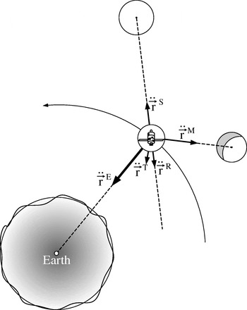
Figure 2. GNSS satellites' significant perturbing accelerations.
Integrating (4) is a cumbersome and complex problem, as the quantity between the brackets depends on the satellite position; in other words, the satellite position vector ![]() is the quantity which must be determined first from the solution of differential equation (4), as a function of time. The usual way to do this is to determine the satellite coordinates in un-perturbed motion and then to adjust them, taking into account the acting perturbations. Here, the un-perturbed motion is seen as a reasonable simplification of the real motion of the satellite and it is often called intermediate motion. Two solutions are applied to evaluate this adjustment:
is the quantity which must be determined first from the solution of differential equation (4), as a function of time. The usual way to do this is to determine the satellite coordinates in un-perturbed motion and then to adjust them, taking into account the acting perturbations. Here, the un-perturbed motion is seen as a reasonable simplification of the real motion of the satellite and it is often called intermediate motion. Two solutions are applied to evaluate this adjustment:
• Variation of Coordinates. This method ignores the satellite's trajectory, assuming that the coordinates of the satellite are directly perturbed. The differences between the perturbed coordinates and the Keplerian (intermediate) coordinates are computed directly, by numerical integration.
• Variation of Constants. It is assumed that the six constants (2) resulting from analytical integration of differential equation (1) are time dependent functions. Perturbations are regarded as deviations between the Keplerian (intermediate) elements at a given initial epoch (t0) and at a further epoch (t).
The general evaluation of the dynamic behaviour of a GNSS constellation requires a proper choice of instrumentation presented above. A thorough analysis of each element's variation due to each perturbation may be approached by a straight numerical integration and the large databases obtained may offer a platform for further analyses and conclusions, but this is not the aim of this work. Instead, the broad, general dynamic comparison between the three GNSS constellations in this work will be done by an analytical approach, using only those perturbations of significant influence in time.
Intermediate (Keplerian) orbit is, as already presented, a fictitious, ideal path of a satellite; its value is not only theoretical, but also practical: this motion is used as a reference orbit to which the perturbed motion is compared. When perturbations are taken into account, the requirement for orbital elements to be time-dependent is the base for analytical approach and drives us to the osculating elements. Let us assume that at epoch t0 the position vector of a GNSS satellite is ![]() (Figure 3). The motion is further considered unperturbed, so that at epoch t 1 the position vector is un-equivocally determined,
(Figure 3). The motion is further considered unperturbed, so that at epoch t 1 the position vector is un-equivocally determined, ![]() . At this stage the perturbations are evaluated and the orbital elements are corrected accordingly, obtaining the corrected position
. At this stage the perturbations are evaluated and the orbital elements are corrected accordingly, obtaining the corrected position ![]() . The motion is further considered unperturbed with orbital elements imposed by (
. The motion is further considered unperturbed with orbital elements imposed by (![]() ), so that at epoch t 2 the position vector is again unequivocally determined,
), so that at epoch t 2 the position vector is again unequivocally determined, ![]() . After the perturbations in elements are introduced, the corrected position
. After the perturbations in elements are introduced, the corrected position ![]() is obtained. Then, the satellite is again forced to move on a Keplerian orbit with elements determined by
is obtained. Then, the satellite is again forced to move on a Keplerian orbit with elements determined by ![]() . The successive Keplerian orbits whose elements correspond to corrected positions
. The successive Keplerian orbits whose elements correspond to corrected positions ![]() ,
, ![]() , …,
, …, ![]() are called osculating orbits. Basically, the satellite moves on a Keplerian (intermediate) orbit, whose elements modify at every correction step.
are called osculating orbits. Basically, the satellite moves on a Keplerian (intermediate) orbit, whose elements modify at every correction step.

Figure 3. Osculating orbits.
The real, irregular orbit may be regarded as the envelope of all successive osculating orbits (Seeber 1993, p.74). With the time increasing continuously, the real (perturbed) motion of a satellite may be treated as a Keplerian motion with orbital elements varying continuously as functions of time:
For the general evaluation of orbits' behaviour in time intended in this work, only the significant perturbing influences will need to be taken into account, as detailed in Table 1; the main perturbing influence stays with the non-central gravitational field of the Earth, as it exceeds all the other perturbing accelerations at least by factor 103. This main perturbation induces slow variations of orbital elements in time; consequently, it is possible to approximate the orbital elements by a power series in time differences (t−tk):
where p i is any of the six orbital elements (i=1, …, 6) in (2) and t k is a mean epoch. Any osculating element p i may be represented as the sum of long-period and short-period terms (Goad, Reference Goad1977):
with ![]() containing the secular part of an element's variation and Δp i(t) containing the periodic one. The terms
containing the secular part of an element's variation and Δp i(t) containing the periodic one. The terms ![]() are also known as mean elements. It is therefore practical to use in the present investigation mean elements as osculating elements, with vanished periodic parts. The equations that connect the perturbing forces and the time-dependent variations of the orbital elements are those developed by Lagrange (1736–1813), the so-called Lagrange Planetary Equations (LPE), which are based on perturbing potential, ℜ, whose first derivative is the perturbing force. In other words, LPE establish the relationship between disturbing potential ℜ and the variations of the orbital elements.
are also known as mean elements. It is therefore practical to use in the present investigation mean elements as osculating elements, with vanished periodic parts. The equations that connect the perturbing forces and the time-dependent variations of the orbital elements are those developed by Lagrange (1736–1813), the so-called Lagrange Planetary Equations (LPE), which are based on perturbing potential, ℜ, whose first derivative is the perturbing force. In other words, LPE establish the relationship between disturbing potential ℜ and the variations of the orbital elements.
The explicit derivation of LPE can be found in classical textbooks on celestial mechanics, e.g. Brouwer and Clemence Reference Brouwer, Clemence and 1961 or Kaula Reference Kaula1966, as follows:

For orbits with small eccentricities ω becomes indeterminate and for orbits with small inclinations Ω becomes indeterminate; in these situations, in order to avoid singularities, the canonical set of Hill's elements should be used (cf. Brouwer and Clemence Reference Brouwer, Clemence and 1961, p.287), in which Hill's variables are used instead of orbital elements (Figure 4 (Left)), as follows:

with G being a variable (the gravitational constant was incorporated in μ, the gravitational parameter). In other cases, it is practical to express the perturbing acceleration through its rectangular components, in the satellite's position (see Figure 4 (Right)). This is the case when the perturbing force cannot be derived from a potential, the so-called non-conservative perturbing forces, or when we have to treat orbits with large eccentricities. It is also worth mentioning that LPE are less suitable for direct numerical integration. An appropriate alternative is based on Gaussian decomposition of the perturbing force into three orthogonal components (in transposed form):
with S, the radial component, contained in the orbital plane, oriented in the direction of radius vector (![]() ), positive in the direction of increasing of radial distance; T, the normal component, contained in the orbital plane, perpendicular to S component, positive in the direction of increasing longitude; W, the bi-normal component, perpendicular to the orbital plane, positive to the north celestial pole. The corresponding Gaussian relations between perturbation components and time-variations of orbital elements can be found in, e.g. Brouwer and Clemence Reference Brouwer, Clemence and 1961, p.301.
), positive in the direction of increasing of radial distance; T, the normal component, contained in the orbital plane, perpendicular to S component, positive in the direction of increasing longitude; W, the bi-normal component, perpendicular to the orbital plane, positive to the north celestial pole. The corresponding Gaussian relations between perturbation components and time-variations of orbital elements can be found in, e.g. Brouwer and Clemence Reference Brouwer, Clemence and 1961, p.301.

Figure 4. (Left) Hill's variables; (Right) Gaussian perturbing force components.
In the systems above the following variables were used: ν, E, M are true, eccentric and mean anomaly respectively, u=ω+ν is the satellite's argument of latitude and p is the ellipse parameter given by: p=r·(1+e·cosν).
QUALITATIVE INVESTIGATION OF GNSS SPACE SEGMENT BEHAVIOUR
Perturbations caused by geopotential
Clearly, the dominant perturbation on GNSS satellites comes from the non-central gravitational field of the Earth; in practical terms, the Earth's equatorial mass excess produces a torque which rotates the satellite's orbit in the equatorial plane, producing a nodal regression ![]() . Also, a second effect of the non-central geo-potential causes the orbital perigee to migrate
. Also, a second effect of the non-central geo-potential causes the orbital perigee to migrate ![]() . Analytical investigation of these phenomena is based on the development of perturbing geo-potential into spherical harmonics:
. Analytical investigation of these phenomena is based on the development of perturbing geo-potential into spherical harmonics:
(cf. Heiskanen and Moritz 1967, p.342), where the term ![]() represents the spherical Earth's potential, whose gradient
represents the spherical Earth's potential, whose gradient ![]() is the central attractive acceleration in the Keplerian motion, 104 times bigger than the sum of all perturbing accelerations. This difference was first converted in orbital (osculating) elements by Kaula, Reference Kaula1966, p.30–37, being useful to develop the analytical integration of EPL. Coefficients C ℓm and S ℓm are named according to the following rule: when m=0, they are called zonal coefficients; when m≠0, tesseral coefficients; and when m=l, sectorial coefficients. The time-dependent variations of the perturbations are described by Kaula's function S ℓmpq(ω, Ω, M, θ), where θ is the Greenwich sidereal time; consequently, the nature of the perturbations produced by the non-central geopotential is imposed by the temporal behaviour of these arguments, following the equation, which covers the whole spectrum of frequencies generated from combinations of l, m, p, q terms:
is the central attractive acceleration in the Keplerian motion, 104 times bigger than the sum of all perturbing accelerations. This difference was first converted in orbital (osculating) elements by Kaula, Reference Kaula1966, p.30–37, being useful to develop the analytical integration of EPL. Coefficients C ℓm and S ℓm are named according to the following rule: when m=0, they are called zonal coefficients; when m≠0, tesseral coefficients; and when m=l, sectorial coefficients. The time-dependent variations of the perturbations are described by Kaula's function S ℓmpq(ω, Ω, M, θ), where θ is the Greenwich sidereal time; consequently, the nature of the perturbations produced by the non-central geopotential is imposed by the temporal behaviour of these arguments, following the equation, which covers the whole spectrum of frequencies generated from combinations of l, m, p, q terms:
cf. Arnold 1970, Seeber 1993 p.83, where Ψ is an angular argument. From particular combinations of l, m, p, q in Equation (12) a few preliminary conclusions may be drawn:
• Simultaneous condition l−2p=l−2p+q= m=0 leads to
 =0. This indicates that only zonal coefficients C ℓ0 (in Equation 11) produce secular perturbations in some orbital elements. Secular perturbations are time cumulative, rather linear, variations of certain orbital elements with an important impact on the space segment of GNSS general dynamics and stability. Moreover, the influence of tesseral and sectorial harmonics are much smaller and therefore neglected in the present study;
• Simultaneous conditions: l−2p≠0; l−2p+q=0 and m=0 in Equation (12) lead to long-period perturbations, i.e. variations of orbital elements with period longer than 100 days. These variations are produced by zonal harmonics (J20 in principal).
• Simultaneous conditions l−2p+q≠0 and/or m≠0 yield in short-periodic perturbations; these are orbital elements' variations with periods comparable with satellite orbital period.
The analytical approach permits not only the dissemination among types of perturbations, but also a numerical evaluation of the magnitude of these perturbations. This attempt may offer the possibility of evaluating the secular perturbations which may permit us to draw some conclusions on how stable in time one space segment or another would be.
Making l=2, m=0, p=1, q=0 in the basic relation of disturbing potential caused by the non-central attraction field of the Earth (Equation 11) and replacing this potential in LPE (Equation 8) will result in the following simplified system:

in which a e is the equatorial radius of the ellipsoidal model of the Earth, n is the mean angular velocity of the satellite on orbit (with n=2·π/P=(μ/a 3)1/2, where P is the orbital period of the GNSS satellite), a is the semi-major axis of the satellite orbit, e and i are the orbital eccentricity and inclination respectively and J 2=−C 20=−1082·63⋅10−6 is the coefficient of the second (zonal) harmonic of the geo-potential. As this harmonic exceeds all others harmonics of the geopotential at least 1000 times, the main conclusions – in quantity terms – may be further produced by numerical calculus, with known numerical values of the above parameters; thus, we may evaluate rather accurately the secular variations of the three orbital parameters (Ω, ω, M) affected only by the significant part of the geo-potential, namely the second (zonal) harmonic.
With average values for GNSS orbital semi-major axis (a GPS≅26560 km; a GLONASS≅25480 km; a GALILEO≅29600) and eccentricity (e≅0), we may estimate the impact of orbital inclination in the secular nodal precession of GNSS orbits due to the greatest Earth's gravitational perturbing influence, namely the second zonal harmonic (J2). The results in Table 2 will be re-found on Figure 8, being in close accordance with systems' specifications (e.g. GLONASS Interface Control Document, version 5.0, pp.34). Using the same values for a and e, the reference rate of the perigee motion of a GNSS satellite are shown in Table 3.
Table 2. Reference values of secular precession of GNSS ascending node produced by J2.

Table 3. Reference values of secular precession of GNSS perigee produced by J2.

Perturbations due to Sun/Moon gravitational attraction
Assuming that the Sun and the Moon are mass-points, as is the case with the satellite, the basic Equation (3) may be used to evaluate the Sun/Moon perturbing accelerations acting against a GNSS satellite (Seeber 1993, p.88):

With GM S≅1325·108 [km3/s2] and GM M≅49·102 [km3/s2] a numerical evaluation of the perturbations in coordinates may be approached, provided a ephemeris of Sun and Moon are available at every step of the numerical integration algorithm (Cojocaru, Reference Cojocaru2007). To obtain a holistic view of the gravitational influence of the Sun and the Moon on mean GNSS orbits, the analytical approached must be adopted; similar to geopotential, the perturbing potential of the Sun and Moon must be expressed in orbital elements and then substituted in the EPL system (8). Resulting analytical expressions of secular variation of ω and Ω were given by Kozai (Reference Kozai1959) ; other orbital parameters (a, e, I, ω, Ω) are subject to short periodic perturbations, derived by e.g. Kozai Reference Kozai1966, Giacaglia 1973.
Other perturbations
Solid earth and ocean tides modify the geopotential and act subsequently as additional perturbations against an average GNSS orbit; however, this is an indirect gravitational effect and is much weaker than the previous ones (e.g. for GNSS orbits, the perturbing acceleration is 10−9 m/s2, which induces long periodic variations of Ω and i); further, in GNSS satellites' positions, the magnitude of this effect is less than 1 m in 4 orbital periods (cf. Lambeck et.al.Reference Lambeck, Cazenave and Balmino1975). Solar radiation pressure acts as a disturbing influence against a mean GNSS satellite orbit causing a perturbing acceleration of 10−7 m/s2. Resulting variations of orbital elements are extremely difficult to evaluate as the perturbing force does not result from a potential and EPL cannot be applied. Furthermore, the perturbing force is a non-continuous function, as GNSS satellites pass through successive light-penumbra-umbra zones. Numerical approaches are suitable, based on a cylindrical shadow-model and a body/fixed satellite coordinate system.
CONCLUSIONS
The effects of perturbations on the motion of GNSS satellites are imposed by the amplitude of their mean osculating elements. Figure 5 offers a broad image of the impact of the most significant perturbations on orbits of various size (given by semi-major axis, a). Compared to close-Earth orbit satellites, GNSS (MEO) orbits are less affected by Earth's gravitational influence, while a greater influence of Sun/Moon attraction and solar radiation pressure is recognized. Inside GNSS, the higher the altitude of the satellite, the more stable orbit is recorded. From this point of view, GALILEO mean orbits are more stable.

Figure 5. Perturbing effect on orbits of different size (after Landau et.al Reference Landau and Hagmeier1986).
However, the main important difference between existing GNSS is dictated by the orbital inclination. The main perturbing influence is represented by the second zonal harmonic of the geopotential (of coefficient J2). From the whole spectrum of J2-related perturbations, the secular ones are crucial for the evaluation of time-stability of a GNSS constellation; in this sense, Figures 6 and 7 shape the difference of nodal stability between close Earth orbits and GNSS orbits: the latter are, on average, 100 times more stable.

Figure 6. The order of magnitude of the secular precession of the ascending node for close Earth satellites (after Bate et.al. Reference Bate, Mueller and White1971).
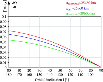
Figure 7. GNSS satellites' ascending node secular precession: a comparative view.
The impact of J2 portion of the geopotential in the GNSS nodal stability is detailed in Figure 8. Obviously, GLONASS orbits are more stable due to the higher orbital inclination.

Figure 8. Impact of GNSS orbital inclination on nodal secular precession due to the second zonal harmonic of the geopotential.
Orbital size and inclination prove to be crucial for the perigee secular precession. Figures 9 and 10 comparatively present the magnitude of perigee precession for close and medium orbits: as one can easily observe in Figure 11, GLONASS orbits are more stable due to their inclination being much closer to the critical inclination (as also concluded by Equation 12).
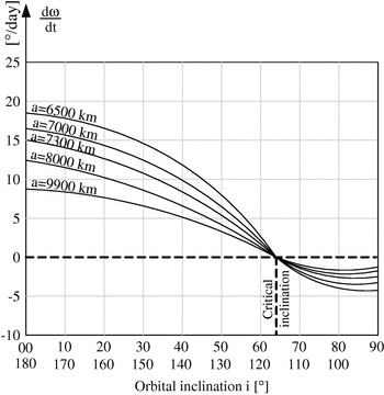
Figure 9. The order of magnitude of the secular precession of perigee for close Earth satellites (after Bate et.al. Reference Bate, Mueller and White1971).

Figure 10. GNSS satellites' perigee secular precession: a comparative view.
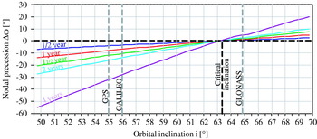
Figure 11. Impact of GNSS orbital inclination on perigee secular precession due to the second zonal harmonic of the geopotential.
Far from completeness, the conclusions presented above are based on numerical simulations of analytically deduced Equations (8), in simplified form (13). They are materialized in Figures 8 and 11, which strongly suggest that a yearly manoeuvre to re-adjust the GNSS satellite position in its orbit should be necessary; however, periodic perturbations have not been taken into account, lacking significance over long-term orbital stability.
ACKNOWLEDGEMENT
The author is grateful to Dr. Vasile Mioc, Director, Romanian Astronomical Institute the authority that supported the research partially covered in this work. Also, the precious help and continuous encouragement from Commander David M. Vaughan, OBE, FRIN, Royal Navy, are gratefully acknowledged.


