1. INTRODUCTION
Current techniques and algorithms employed for Receiver Autonomous Integrity Monitoring (RAIM) have evolved from single epoch snapshot solutions. The extensive demand for kinematic GNSS positioning, however, has led to a derivation of statistical quality control principles, based on the least squares residuals, for the Kalman filter. The Kalman filtering technique is widely accepted to provide optimal estimates of the navigation parameters of a dynamic platform, assuming the state and observation models are correct. Unfortunately, such assumptions do not always hold and inevitably, significant deviations from the assumed models are not uncommon for dynamic systems. If the assumptions for the mathematical models are correct, the state parameter estimates are unbiased with a minimum variance within the class of linear unbiased estimators. Unpredictable events, such as multipath in the GNSS measurements or the deviation of receiver dynamics from the assumed dynamic model, result in unmodelled errors. In order to detect and account for such errors the state estimation procedure must be complemented with effective quality control techniques, such as RAIM. The RAIM performance should also be assessed in its ability to alert the user when the solution cannot be guaranteed to meet the specified performance tolerances. The assessment should include both reliability and separability measures, where reliability is an assessment of the capability of GNSS receivers to detect outliers and separability refers to the system's ability to correctly identify the detected outliers from the measurements. In kinematic positioning scenarios RAIM procedures should also be capable of detecting and identifying faults due to mis-modelling of the system dynamics.
Developments in quality control and RAIM algorithms for kinematic GPS have progressed at an impressive rate over the last decade. Quality control for integrated navigation systems using recursive filtering is described in Teunissen (Reference Teunissen1990). Lu (Reference Lu1991) uses a two-stage Kalman filter (Friedland, Reference Friedland1969; Ignagni, Reference Ignagni1981) for differential kinematic GPS quality control including reliability determination. In Salzman (Reference Salzmann1995) a procedure for real-time adaptation for model errors in dynamic systems is presented and analysed. Gillesen and Elema (Reference Gillesen and Elema1996) present the results of a detection, identification and adaptation (DIA) procedure with reliability analysis in a kinematic integrated navigation system. DIA and reliability evaluation techniques for kinematic GPS surveying are discussed in great detail in Tiberius (Reference Tiberius1998b) and Nikiforov (Reference Nikitorov2002) discusses integrity monitoring with fault detection and exclusion (FDE) algorithms for integrated navigation systems.
In this paper, the algorithms for the RAIM of a dynamic GNSS receiver derived from the least squares estimators of the state parameters in a Gauss-Markov Kalman filter (Wang et al., Reference Wang, Stewart and Tsakiri1997) are used to assess the impact of dynamic information via a Kalman filter on GNSS RAIM. Herein, the dynamic information is delivered via velocity estimates derived from the accumulated delta range measurements. Analyses compare the outlier detection and identification capabilities and reliability and separability measures of a GPS-only system, with and without the delta-range measurements.
2. GNSS NAVIGATION MODELS
2.1. Kalman Filtering in GNSS Navigation
A discrete extended Kalman filter (EKF), where the measurement models are linearised about an approximation of the state at discrete time intervals, is typically used for GNSS navigation solution estimation. For standalone GNSS navigation, either an 8-state or 11-state filter is generally employed depending on the dynamics of the system. If the dynamics are relatively low, such as in a car or less mobile vehicle, the 8-state filter estimating only the position, velocity and clock bias and drift may be sufficient. In this case, the accelerations are assumed to be white noise and are therefore accounted for in the system process noise. However, if the system is expected to experience high dynamics with significant accelerations an 11-state filter incorporating the implicit estimation of the accelerations should be used.
Regardless of the number of states employed, the state evolution model of the discrete extended Kalman filter describes the dynamic processes of the system:
and the linearised measurement model relates the measurements to the state of the system:
where  is the m k×1 updated state parameter vector at epoch k−1; is the m k×1 predicted state vector for epoch k made at epoch k−1; Φk,k−1 is the m k×m k−1 state transition matrix from epoch k−1 to k; w k is the m k×1 random error vector representing the dynamic process noise at epoch k; z k is the n k×1 measurement vector at epoch k; H k is the n k×m k geometry matrix relating the measurements to the state parameters and εk is the n k×1 error vector of the measurement noise at epoch k.
2.2. GNSS Navigation Dynamic Models
The 8-state filter is based on a Position-Velocity (PV) model where the acceleration is assumed as white noise and the velocity and position are estimated as random-walk processes (Brown and Hwang, Reference Brown and Hwang1996). The 8-state vector for the PV model is:
The 11-state filter is based on a PVA model where the acceleration can be estimated as either a random-walk or a Markov process. Theoretically, the stationary Gauss-Markov model may generally be more appropriate than the non-stationary random-walk model as accelerations are rarely sustained (Brown and Hwang, Reference Brown and Hwang1996). For this reason, the Gauss-Markov model was adopted for the simulations herein. For the Gauss-Markov PVA model, the acceleration is modelled as a Gauss-Markov process with parameter where tẽ is the system acceleration. The 11-state vector of the PVA model is:
For details regarding the transition and process noise covariance matrices used herein, readers are referred to Brown and Hwang (Reference Brown and Hwang1996).
2.3. Kalman Filtering as Least Squares
A major advantage of the snapshot solution for GNSS navigation is that, unlike the Kalman filter, it is not model dependent. Due to this model dependence, the solutions of Kalman filter-based integrity algorithms are prone to high false alarm rates when unexpected system dynamics are experienced. The Kalman filter residual vector, or innovation sequence, only gives the residuals corresponding to the measurements with respect to the state predictions and not a posteriori residuals of both the measurements and state predictions. Therefore, by performing a least squares navigation solution containing the measurements and the predicted states of the Kalman filter's dynamic model, we can obtain an ideal integrity solution which not only checks the consistency of the measurements but also the state predictions.
It has been shown that by integrating the measurements z k with the predicted values of the state parameters , optimal estimates for the state parameters x k can be obtained using least squares principles. The corresponding measurement model is (Sorenson, Reference Sorenson1970; Cross, Reference Cross, Hawksbee and Nicolai1987; Salzmann, Reference Nikitorov1993; Leahy and Judd Reference Leahy and Judd1996; Wang et al, Reference Wang, Stewart and Tsakiri1997):
where . l k is the least squares measurement vector containing measurements z k and predicted state parameters ; A k is the (n k+m k)×n k design matrix; v zk is the n k×1 residual vector of the measurements z k; is the n k×1 residual vector of predicted state parameters ![]() k; E is the m k×m k identity matrix.
k; E is the m k×m k identity matrix.
The corresponding stochastic model is described as:
where Cl k is the VCV of the measurement vector l k. The optimal estimates for the state parameters and the error covariance matrix can be determined by:
The filtering residuals v yk and can then be calculated from:
From the least squares principles the cofactor matrix of the filtering residuals is:
3. RAIM ALGORITHMS
Through adopting least squares principles for the state estimations in a Kalman filter, the same quality control algorithms as for the single epoch snapshot approach can be used. In such a case, the predicted state parameters can be included as measurements in the adjustment. The algorithms used herein are based on the widely known and implemented detection, identification and adaptation (DIA) procedure. For a detailed background to the DIA procedure used herein, see Wang and Chen (Reference Wang and Chen1994) and Hewitson et al. (Reference Hewitson, Lee and Wang2004). The inclusion of dynamic information, in the form of the state parameter predictions of the Kalman filter, increases the redundancy of the adjustment. The improvement in redundancy has significant effects on the quality control.
3.1. Outlier Identification
Once a fault has been detected with a global detection algorithm such as the variance factor test, the w-test can then be used to identify the corresponding measurement, where the test statistic is (Baarda, Reference Baarda1968; Cross et al., Reference Cross, Hawksbee and Nicolai1994; Teunissen, Reference Teunissen, Teunissen and Kleusberg1998):
Under the null hypothesis, w i has a standard normal distribution and under the alternative, w i has the following non-centrality:
The critical value for the test is N 1−α/2(0,1), where α is the significance level.
3.2. Reliability
The internal reliability is expressed as a minimal detectable bias (MDB) and specifies the lower bound for detectable outliers with a certain probability and confidence level. The MDB is determined, for correlated measurements (Baarda, Reference Baarda1968; Cross et al., Reference Cross, Hawksbee and Nicolai1994), by:
where δ0 is the non-centrality parameter, which depends on the detection probability and false alarm rate. The external reliability is then evaluated as (Baarda, Reference Baarda1968; Cross et al., Reference Cross, Hawksbee and Nicolai1994):
3.3. Separability
For situations arising where an outlier is sufficiently large to cause many w-test failures, resulting in many alternatives, it is essential to ensure any two alternatives are separable so that a good measurement is not incorrectly flagged as an outlier. The probability of incorrectly flagging a good measurement as the detected outlier is dependent on the correlation coefficient of the test statistics w i and w j (Förstner, Reference Förstner1983; Wang and Chen Reference Wang and Chen1994; Tiberius, Reference Tiberius1998a):
where |ρij|⩽1. Correlation coefficients of 1 and 0 correspond to full and zero correlation between two test statistics, respectively. The greater the correlation between two test statistics, the more difficult they are to separate. The degree of correlation of measurements is dependent on the measurement redundancy and geometric strength. If the measurement redundancy is equal to 1 an outlier can be detected but not identified as all the measurements are fully correlated. When determining the separability, it suffices to only consider the maximum correlation coefficient ρij max(∀j≠i) for each statistic.
4. SIMULATIONS AND RESULTS ANALYSIS
The reference trajectories in Figures 1 and 2 were used to simulate the GNSS measurements of a moving receiver. The measurement update rate was 1 Hz and single frequency pseudorange and accumulated delta range measurements were generated using a modified version of the GPSoft® Satellite Navigation and Navigation System Integration and Kalman Filter Toolboxes. The pseudorange and accumulated delta range measurements are generated with standard deviations of 1 m and 0·1 m, respectively. Accumulated delta-range measurements are taken 50 milliseconds prior to the filter update time as well as at the filter update time to derive the delta-range observables. The delta-range measurements were then used to estimate the receiver's velocity and provide the dynamic information in the Kalman filter for the state predictions. The satellite coordinates were calculated from the Keplerian elements of the nominal 24-satellite constellation design of GPS and all simulations were conducted with a 5-degree masking angle unless stated otherwise.
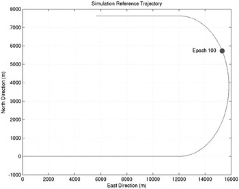
Figure 1. 2D Dog-leg simulation reference trajectory.

Figure 2. 3D Simulation Reference Trajectory.
In order to assess the impact of dynamic information on receiver integrity several scenarios were considered. Firstly, the outlier detection and identification ability of an ordinary least squares (OLS) integrity solution was compared with the Kalman filter solutions of varying weights for the dynamic model. For these comparisons a simple high velocity 2-Dimensional dog-leg trajectory was simulated. Finally, to appropriately investigate the impact of the dynamic information and provide a holistic analysis of the effect of accurately modelled dynamic information on the reliability and separability performance measures a low dynamic 3-Dimensional trajectory was used.
In the following simulations, four variations of the extended Kalman filter (EKF) were used; EKF1-3 use the random-walk PV model and EKF4 is based on the Gauss-Markov PVA model. The spectral amplitudes used for each model are shown in Table 1 along with the correlation time constant parameter for the acceleration state, where S p, S f and S g are the spectral amplitudes associated with the white noise driving functions corresponding to the position, clock bias and clock drift estimates respectively (Brown and Hwang, Reference Brown and Hwang1996). In order to maintain a similar weight with respect to the position state of EKF3, the Sp of EKF4 was set to 67. All the integrity solutions used in the following analyses were derived from the least squares principles and the critical value used for the w-test was 3·2905 for a significance level (α) of 0·1%. The internal reliabilities (MDBs) were determined with a detectability (γ) of 80% and a false alarm rate (significance level, α) of 0·1%.
Table 1. Process noise covariance parameters for Kalman filter adjustment models.

4.1. Single Epoch Outlier Identification Performance Analysis
In this section, the dog-leg trajectory in Figure 1 was used to compare the performances of the OLS and EKF estimations with respect to outlier detection and identification. Initially, analyses of all five estimation approaches were made with a single 17m outlier induced into one of the pseudorange measurements of epoch 100 (see Figure 1). Due to space constraints only the results for the OLS, EKF2 and EKF3 scenarios are presented in this section. The position estimation errors and w-statistics for the entire trajectory were then examined and the correlation coefficient matrices corresponding to epoch 100 were also compared. Further outlier identification analyses were then made after increasing the masking angle to 10 degrees, for which only 6 satellites were visible at epoch 100. The measurements were simulated for a receiver moving along the trajectory in Figure 1 with a speed of 200 m/s and a turn-rate of 3 deg/sec. The centripetal acceleration was approximately 10·472 m/s2 and the Kalman filter was updated at 1 Hz.
4.1.2. Ordinary Least Squares (OLS) Estimation
Figure 3 shows the position and clock bias errors of the OLS estimation with respect to the reference trajectory. In this scenario there were 8 satellites visible. It can be clearly seen that the 17m bias induced into the pseudorange to SV11 has caused a 6m error in the Z component of the position. In Figure 4, which shows the w-test statistics for the duration of the simulation, the failure is prominent and has caused several statistics to exceed the critical value of 3·2905 as indicated by the solid red line. Furthermore, we can see that there are some other small w-test failures e.g. near epochs 35 and 90. These errors are not specifically induced and are the results of the measurement noise.

Figure 3. OLS estimation position and clock bias errors.

Figure 4. OLS estimation w-test statistics (α=0·1%, Critical Value=3·2905).
Figure 5 is a visual representation of the correlation matrix for the w-test statistics of epoch 100. Observations 1–8 correspond to the pseudoranges and observations 9–16 correspond to the delta-range measurements. The matrix is symmetric about the diagonal of ones showing that each observation is fully correlated to itself. By definition, this is always true. Generally speaking, the correlations for this adjustment are relatively high although they would be even higher with fewer satellites. It can also be seen that there is no correlation between the pseudoranges and the delta ranges. Furthermore, the pseudoranges are correlated to each other in exactly the same way as the delta-ranges are due to the identical measurement geometries. Regardless of the relatively high correlations, the largest test failure correctly corresponds with the pseudorange to SV11 and has therefore correctly identified the outlier. However, when we increase the masking angle to 10 degrees where there are only 6 satellites in view the reduction in redundancy has a drastic effect on the outlier identification.

Figure 5. Correlation coefficients for epoch 100 of the OLS estimation with 8 satellites visible, ρ∊[0,1].
Table 2 shows the MDBs, w-statistics and maximum correlation coefficients for each measurement when the masking angle is increased to 10 degrees. In this case a single 15 m outlier has been included in the pseudorange to SV15. Here we can see that four statistics have failed the test due to the high measurement correlation. As it is common practice to exclude only the largest w-test failure as the outlier, the outlier has been falsely identified due to the extreme correlation between the test statistics corresponding to the pseudorange measurements to SVs 12 and 15. It can also be seen that there has been a drastic increase in the correlations due to the reduction in redundancy when compared with Figure 5. Table 2 also shows the adjustment after the satellite corresponding to the incorrectly identified fault SV12 has been removed. Here we can see that the w-statistics for the pseudoranges are equal and fully correlated to one another, as are the delta-ranges. In this situation, there is no chance of identifying the remaining or any further faults.
Table 2. Internal reliabilities and simulation results for identifying a +15m outlier induced in Δρ15 by OLS Estimation with 10 degree mask angle (γ=80%, α=0·1%, CV=3·2905).
4.1.3. Extended Kalman Filter Estimation 2 – PV model
The EKF2 adjustment is less affected by the 17m outlier than the OLS adjustment. The position error in the Z component is now 5m, see Figure 6. Figure 7 shows that the outlier is clearly identified in the measurement model and the largest failure correctly corresponds to SV11. Furthermore, the correlation matrix in Figure 8 shows a slight decrease in the pseudorange measurement correlations amongst themselves and a slight increase in the correlations of the predicted states with themselves and the measurements. The correlations amongst the delta-ranges are the same.

Figure 6. EKF2 estimation position and clock bias errors.

Figure 7. EKF2 estimation w-test statistics for measurements (top) and predicted states (bottom), (α=0·1%, Critical Value=3·2905).

Figure 8. Correlation coefficients at epoch 100 of the EKF2 (PV model) estimation with 8 satellites visible, ρ∊[0,1].
Table 3 shows that the 15m outlier in the 10 degree mask angle scenario has now caused four pseudorange and one predicted state w-statistics (predicted Z component of the position error state) to fail due to the increase in correlations of the predicted states with the measurements. The outlier has again been correctly adjusted and after SV15 has been removed there is still the potential to be able to identify another bias even though only five SVs are available. However, it should be remembered that the ability to correctly identify further outliers is limited due to the high correlations. The marked improvement of the MDBs on the OLS estimation should also be noted.
Table 3. Internal reliabilities and simulation results for identifying a +15m outlier induced in Δρ15 by EKF2 Estimation with 10 degree mask angle (γ=80%, α=0·1%, CV=3·2905).

4.1.4. Extended Kalman Filter Estimation 3 – PV model
Figure 9 shows that with the increased weight of the dynamic model for EKF3, the position error in the Z component, due to the 17m outlier, has been decreased to 4m. Figure 10 reveals that once again the outlier has been detected in the measurement model but also that failures are detected in the predicted states at epochs 100 and 123. However, at epoch 100, the largest test statistic corresponds correctly to the pseudorange to SV12. At epoch 123 the failures occur in the statistics corresponding to the predicted states only. These failures are due to a deviation of the system from the dynamic model. At epoch 123 the system is just coming out of turn and this particular deviation has little impact on the position solution as can be seen in Figure 9. The correlation matrix in Figure 11 shows a solid decrease amongst the pseudorange measurement correlations and again, the correlations amongst the delta-range statistics are the same while those between the pseudorange and the predicted state statistics have significantly increased.

Figure 9. EKF3 estimation position and clock bias errors.

Figure 10. EKF3 estimation w-test statistics for measurements (top) and predicted states (bottom), (α=0·1%, Critical Value=3·2905).

Figure 11. Correlation coefficients for epoch 100 of the EKF3 (PV model) estimation with 8 satellites visible, ρ∊[0,1].
4.2. Comprehensive 3D Trajectory Performance Analysis
In order to assess the impact of the dynamic information of outlier detection and identification in a more holistic way, the 3D reference trajectory shown in Figure 2 was used to simulate the GNSS measurements and determine the associated internal reliabilities and maximum correlation coefficients. The measurements were simulated for a receiver with a speed of approximately 4·7 m/s after accelerating from rest at approximately 0·12 m/s2. The centripetal acceleration was approximately 0·34 m/s2 for all turns and the Kalman filter was updated at 1 Hz, 7–8 satellites were visible for the duration of the simulation. Histograms of the internal reliabilities and maximum correlation coefficients were then generated to show the distribution of values over the whole trajectory. The histograms were separated with respect to the pseudorange and delta range measurements and the predicted states for each estimation scenario. It should be noted that the correlation coefficient results were not isolated to type of measurement being analysed due to space limitations, i.e. the results for the pseudorange measurements include the correlations with the delta range and predicted state statistics as well as the statistics corresponding to the other pseudoranges.
Figures 12 and 13 show the histograms of the internal reliabilities and maximum correlation coefficients corresponding to the pseudorange observations for each of the estimation scenarios. It is clear that with the inclusion of the dynamic model and its increasing weights the internal reliabilities and correlation coefficients are improved. Furthermore, with the inclusion of acceleration estimation in EKF4 there is marked improvement in the internal reliabilities though the maximum correlation coefficients appear worse. The greater degree of maximum correlations is due to an increase in correlation between the pseudorange and predicted state statistics. The pseudorange statistics are actually less correlated with the other measurement statistics.

Figure 12. Histogram of pseudorange internal reliabilities for OLS and EKF1-4 estimations (γ=80%, α=0·1%).

Figure 13. Histogram of maximum correlation coefficients corresponding to pseudoranges for OLS and EKF1-4 estimations, ρ∊[0,1].
Figures 14 and 15 are the histograms of the MDBs and maximum correlation coefficients, respectively, associated with the delta range measurements. For the MDBs we can see that there is some improvement in the maximum MDB values with the inclusion and increasing weight of dynamic information. However, the inclusion of the acceleration state estimation has no impact on the MDBs. The correlation results exhibit a substantial degree of decorrelation with the inclusion of the dynamic model although increasing the weight of the dynamic model has little impact on the maximum correlations of the delta-range statistics. The EKF3 and EKF4 results are almost identical.

Figure 14. Histogram of delta range internal reliabilities for OLS and EKF1-4 estimations (γ=80% α=0·1%).

Figure 15. Histogram of maximum correlation coefficients corresponding to delta ranges for OLS and EKF1-4 estimations, ρ∊[0,1].
In Figure 16 it is clear that increasing the weight of the dynamic model improves the MDB values for the state predictions. However, when the acceleration state is estimated there is an improvement in the predicted states except for the velocity predictions which have slightly larger MDBs for EKF4. It should also be remembered that the MDBs for the acceleration states are infinite due to the fact that the acceleration states are unobservable. With respect to the correlations of the predicted state statistics, it is clear from Figure 17 that the maximum correlation coefficients decrease with the increasing weight of the dynamic model but are actually at their largest with the inclusion of the acceleration estimation (EKF4).

Figure 16. Histogram of predicted state internal reliabilities for EKF1-4 estimations (γ=80%, α=0·1%).

Figure 17. Histogram of maximum correlation coefficients corresponding to predicted states for EKF1-4 estimations, ρ∊[0,1].
5. CONCLUSIONS
In this paper, the RAIM algorithms for a dynamic GNSS receiver derived from the least squares estimators of the state parameters have been employed with a Gauss-Markov Kalman filter to evaluate the impact of dynamic information on GNSS RAIM. The actual analyses have been carried out to compare the outlier detection and identification capabilities and reliability and separability measures of a GPS-only system, with and without the delta-range measurements and with varying weight for the dynamic model where applicable.
Based on the results presented here it is clear that RAIM performance can be significantly improved with the inclusion of a dynamic model. The degree of such improvement is dependent on the weighting of the dynamic model. A major advantage of increasing the weight of dynamic model is the drastic improvement in outlier detection and identification robustness in the measurement domain. Furthermore, by performing a least squares navigation solution containing the measurements and the predicted states of the Kalman filter's dynamic model, it has been shown that the dynamic modelling errors can be separated from the measurement errors. However, a drawback to increasing the weight of the dynamic model is that it generates greater levels of correlations between the measurement and the state prediction statistics. In order to reliably distinguish measurement errors from the dynamic modelling errors the correlation coefficients between them must be reasonably low. To gain deeper understanding of the difference between the PV model and the PVA model filters in GNSS RAIM, more investigations are required to determine the effect of any possible benefits of including the estimation of acceleration in the dynamic model.