


1. INTRODUCTION
A pulsar is a high-speed rotating neutron star that radiates electromagnetic waves of various wavelengths periodically to the surroundings. The navigation method that uses one or more pulsars as a signal source is called pulsar navigation. As a new type of autonomous navigation, it has attracted wide attention from scholars all around the world (Becker et al., Reference Becker, Bernhardt and Jessner2013; Xu et al., Reference Xu, Wang, Feng, Jiang, You and He2018a, Reference Xu, Wang, Feng, You and He2018b; You et al., Reference You, Wang, He, Xu, Lu and Feng2018). Pulsar navigation uses the pulsar's periodic electromagnetic waves as the signal source to obtain the position and time information by calculating the phase of the signal. There are three problems in the process of processing this signal. First, because the universe contains a lot of background noise, and the signal detector itself contains noise caused by dark current, etc., the pulse contour obtained contains a lot of noise. Second, the signal of the distant pulsar reaching the detector is very weak and has been attenuated into the form of a single photon. Third, because the effective area of the detector is small, it takes a long time to accumulate. These three problems affect the accuracy of the TOA (Time of arrival) estimate, thereby reducing the accuracy of positioning and punctuality. Consequently, the pulsar signal must be denoised.
The noise reduction method based on wavelet transform has been applied in many fields (Wei et al., Reference Wei, Yue, Wei, Haiyu and Ya2012; Liu et al., Reference Liu, He, Guo and Tang2016). Wavelet transform was applied to the denoising of pulsar signal for the first time in Xiao-ming et al. (Reference Xiao-ming, Fu-cheng and Yuan-yan2006), where the selection of wavelet basis and the number of decomposition layers were studied. That study proved that the wavelet transform could greatly improve the signal-to-noise ratio, and the high-frequency information of the useful signal was not lost. Li et al. (Reference Li, Xi-zheng and Guang-ren2008) studied the selection of the optimal threshold, and selected Coiflets as the wavelet basis for analysing the pulse signal from two angles of tight support and vanishing distance. However, the processing of the threshold does not solve the contradiction between suppressing noise and retaining details. Di et al. (Reference Di, Xu and Zhenhua2007) introduced fuzzy theory into the threshold processing algorithm of wavelet denoising. A membership function was established to distinguish between signals and noise, and noise was suppressed while preserving the signal. In Zhe et al. (Reference Zhe, Xu, Yo, Zhen and Nan2010), an improved wavelet spatial correlation filter denoising method was proposed, that could further improve the ability to preserve signals while suppressing noise. Xue et al. (Reference Xue, Li, Fu, Liu, Sun and Shen2016) proposed a local linear minimum mean square error method for unsampled wavelet domain, that could continue to improve both signal-to-noise ratio and signal retention.
The above scholars mainly focused on the selection of wavelet basis and the design of wavelet threshold function. The choice of wavelet basis is the base of wavelet denoising, so if the selection of the wavelet basis is inappropriate, it will directly affect the denoising effect. There is currently no universal wavelet basis that accommodates all signals, so the most appropriate wavelet basis for different signals is different. In most of the abovementioned literature, the existing wavelet basis was used for the selection of the wavelet basis, and no special wavelet basis was designed for pulsar signals. Few researchers have studied the design of wavelet basis for pulsar signals. Hence, the wavelet basis set CPn (Crab pulsar wavelet basis, where n represents the wavelet basis length) for the pulsar signal is designed in this study. This set of wavelet basis can offer the denoised signal with greater signal-to-noise ratio, and lower mean square error and peak position error.
The rest of the paper is organised as follows. In Section 2, the signal of the Crab pulsar is analysed by the frequency domain method, and then the wavelet basis is designed. Section 3 implements a wavelet lifting algorithm. The simulation carried out is described in Section 4 and the simulation results are analysed. Section 5 gives the conclusion.
2. FREQUENCY DOMAIN ANALYSIS OF PULSAR SIGNAL AND CONSTRUCTION OF WAVELET BASIS
2.1. Analysis of frequency characteristics of pulsar signal
The literature (Fang et al., Reference Fang, Liu, Li, Sun, Xue, Shen and Zhu2016) proves that the TOA estimation can completely abandon the high-frequency part information that experiences the greatest interference from noise, and only uses the low-frequency part information with high signal-to-noise ratio. FFT (fast Fourier transformation) is performed on the actual profile of the Crab pulsar data of the actual period of 1 s and the actual noisy profile obtained by epoch folding, as shown in Figure 1. By comparing the FFT amplitude-frequency curves, it can be seen that the ideal curve mainly concentrates on the low frequency near 0 KHz, and the noise-containing curve has components in the range of 20–40 KHz. When designing low-pass filters, the cut-off frequency should be as close as possible to 0 KHz, and the curve of the filters should be as vertical as possible to the x-axis, so as to approach the ideal filter. The closer to the ideal filter, the higher the order of the filter is required, but the higher the order, the larger the amount of calculation. Therefore, when designing the wavelet basis, the contradiction between the calculation amount (order) and the signal-to-noise ratio should be balanced.
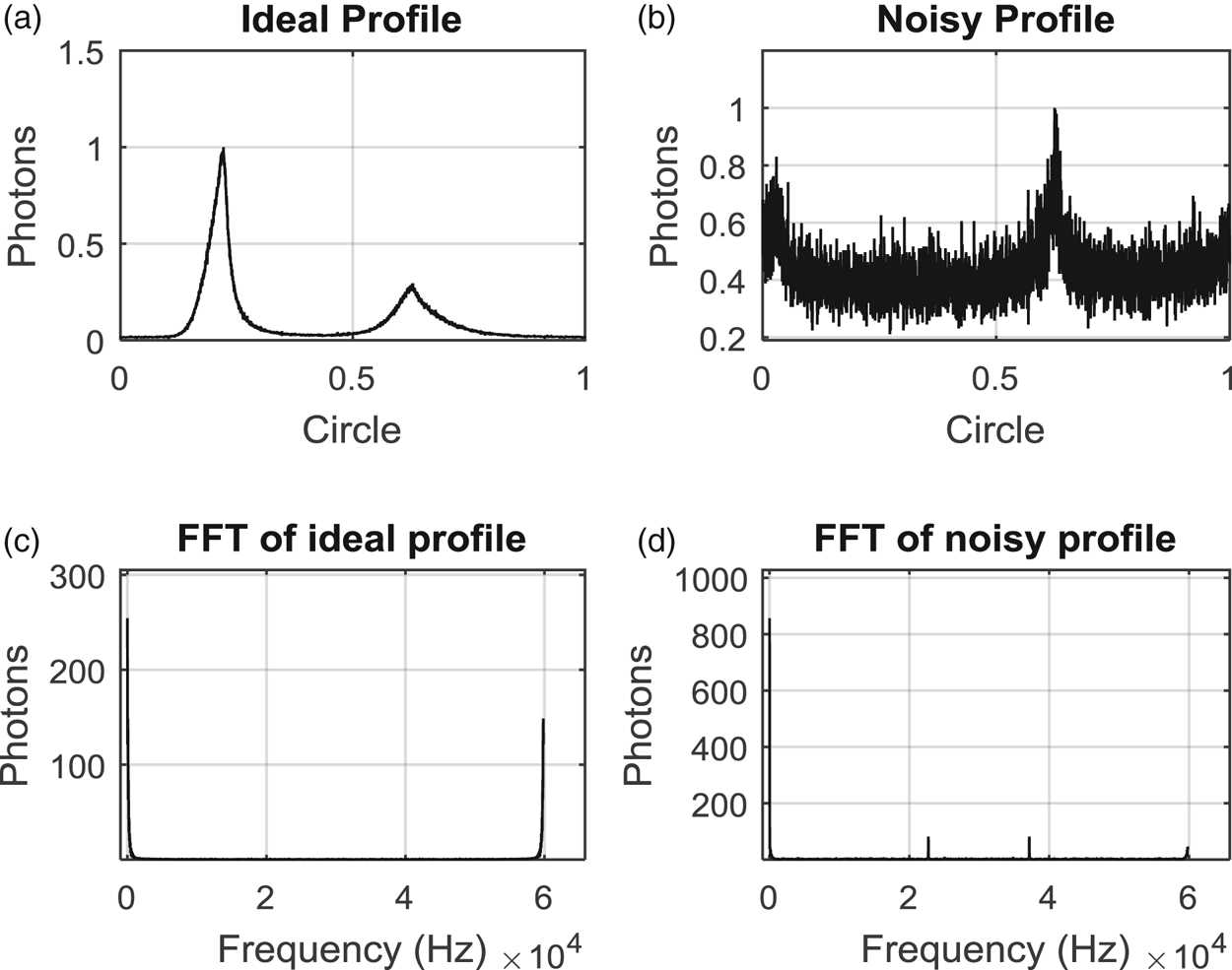
Figure 1. Waveform and FFT transform of ideal profile (a, c) and noisy profile (b, d).
2.2. Construction of wavelet basis
Constructing a wavelet basis requires two principles of linear phase and convergence, for two reasons. First, phase distortion affects the TOA estimation of subsequent pulsar signals, which affects the positioning and punctuality of pulsar navigation. Therefore, the process of pulsar signal denoising cannot be phase-distorted. Secondly, if the filtered curve diverges, the filtering purpose cannot be achieved, and the waveform will also be deformed, so it is desirable that the filtered curve converges.
The CPn wavelet basis cluster is designed by the Hamming window method, which is compared with the Dbn (Daubechies) wavelet basis cluster as shown in Figure 2. n represents half the length of the filter. The larger n is, the better the filtering effect is, and the closer it is to the ideal filter in the frequency domain (as shown in Figure 3). It also demands a larger amount of calculation, however, so a trade-off is required between the amount of calculation and the filtering effect according to the specific engineering requirements.
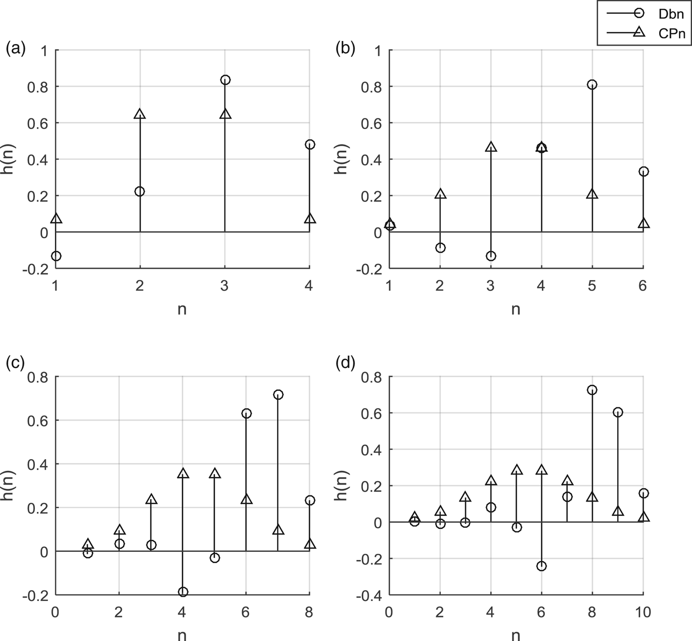
Figure 2. Comparisons of Dbn and CPn wavelet bases of different lengths: (a) 4, (b) 6, (c) 8 and (d) 10.

Figure 3. Comparison of FFT transform of Dbn and CPn wavelet bases of different lengths: (a) 4, (b) 6, (c) 8 and (d) 10.
Figure 2(a)–(d) correspond to Dbn and CPn of lengths 4, 6, 8, and 10. It can be seen from the figure that the coefficients of CPn follow the even or odd symmetry. Therefore, the phase delay and group delay of CPn are equal and constant in the frequency band. For CPn of n-order linear phase, the group delay is n/2. That is to say, the signal after wavelet transform is simply delayed by n/2 steps. This attribute preserves the waveform of the signal in the passband, that is, there is no phase distortion.
The FFT of wavelet basis of lengths 4, 6, 8 and 10, respectively, is shown in the graphs in Figure 3(a)–(d). In the case of the same length, all CPn wavelet basis low-pass filter amplitude-frequency curve hCPn and high-pass filter amplitude-frequency curve gCPn are respectively below Dbn's low-pass filter amplitude-frequency curve hDbn and high-pass filter amplitude-frequency curve gDbn. That is to say, the angle between the curve and the y-axis is smaller. Closer to the ideal filter, in theory, the filtering effect is better.
The pole-zero diagrams of CPn of lengths 4, 6, 8 and 10 are presented in the graphs in Figure 4(a)–(d). It can be seen from the figure that the poles of CPn are all within the unit circle, so they are stable and will not diverge after wavelet transformation.

Figure 4. Zero-pole maps of CPn wavelet basis of different lengths: (a) 4, (b) 6, (c) 8 and (d) 10.
3. IMPLEMENTATION OF LIFTING ALGORITHM
The lifting algorithm is a more flexible and more versatile tool than the traditional wavelet, which is independent of the Fourier transform (Sweldens, Reference Sweldens1998). Because the lifting algorithm first downsamples and then convolutes, it can reduce the complexity of the algorithm by half compared with traditional wavelets. The process of lifting the algorithm is divided into three main steps, as shown in Figure 5.

Figure 5. Basic flow of lifting algorithms.
First step, split
The pulsar profile signal X after epoch folding is divided into two odd and even sets of two vectors X e and X o which do not intersect each other, according to the index value i.
Second step, prediction
Designing the prediction operator  ${\tilde {{\rm s}}}$, combining X e and X o to obtain the prediction bias
  $\tilde {\gamma }$, can be considered as the high-frequency coefficient of X.
Third step, update
Designing the update operator  ${\tilde {{\rm t}}}$, combining
  $\tilde {\gamma }$ and X e, yields the approximation coefficient
  $\tilde {\lambda }$.
The above three steps represent an ideal, but the actual situation may be more complicated. In fact, there may be multiple predictions and updates, and there may be multiple scale-ups, such as K 1 and K 2 in Figure 5. The process of implementing the lifting algorithm for  $\mbox{h}_{\rm{CPn}}$ and
  $\mbox{g}_{\rm{CPn}}$ is as follows.
According to
 $$\begin{aligned} \lambda (z) & =\tilde{{\rm h}}_{\rm{CPn}} (z)X(z) \\ & =\tilde{{\rm h}}_{\rm e} (z)X_e (z)+z^{-1}\tilde{{\rm h}}_{\rm o} (z)X_o (z) \\ \end{aligned}$$
and
 $$\begin{aligned} \gamma (z) & ={\tilde {{\rm g}}}_{\rm{CPn}} (z)X(z) \\ & ={\tilde {{\rm g}}}_{\rm e} (z)X_e (z)+z^{-1}{\tilde {{\rm g}}}_{\rm o} (z)X_o (z), \\ \end{aligned}$$
a matrix form equation
 $$\left[ {{\begin{matrix} \boldsymbol{\lambda} \\ \boldsymbol{\gamma} \\ \end{matrix} }} \right]=\left[ {{\begin{matrix} {{\tilde {\rm h}}_{\rm e} ({\rm z})} & {{\tilde {\rm h}}_{\rm o} ({\rm z})} \\ {{\tilde {\rm g}}_{\rm e} ({\rm z})} & {{\tilde {\rm g}}_{\rm o} ({\rm z})} \end{matrix} }} \right]\left[ {{\begin{matrix} {\boldsymbol{X}_e (z)} \\ {z^{-1}\boldsymbol{X}_o (z)} \end{matrix} }} \right].$$
is obtained. A multiphase matrix
 $$\tilde{{\textbf{\textit{P}}}}=\left[ {{\begin{matrix} {{\tilde {\rm h}}_{\rm e} ({\rm z})} & {{\tilde {\rm h}}_{\rm o} ({\rm z})} \\ {{\tilde {\rm g}}_{\rm e} ({\rm z})} & {{\tilde {\rm g}}_{\rm o} ({\rm z})} \end{matrix} }} \right].$$
can be obtained. According to
 $$\tilde {P}(z)=\left( {{\begin{matrix} {{\tilde {\rm h}}_{\rm e} (\mbox{z})} & {{\tilde {\rm h}}_0 (\mbox{z})} \\ {{\tilde {\rm h}}_{\rm e} (\mbox{z})t(\mbox{z})+{\tilde {\rm g}}_{\rm e}^{\rm{new}} (\mbox{z})} & {{\tilde {\rm h}}_{\rm o} (\mbox{z})t(\mbox{z})+{\tilde {\rm g}}_{\rm o}^{\rm{new}} (\mbox{z})} \\ \end{matrix} }} \right)=\left( {{\begin{matrix} 1 & 0 \\ {{\tilde {\rm t}({\rm z})}} & 1 \\ \end{matrix} }} \right)\tilde {P}^{\rm{new}}(z)$$
and
 $$\tilde {P}(z)=\left( {{\begin{matrix} {{\tilde {\rm h}}_{\rm e} (\mbox{z})+{\tilde {\rm g}}_{\rm e} (\mbox{z}){\tilde {\rm s}}(\mbox{z})} & {{\tilde {\rm h}}_{\rm o} (\mbox{z})+{\tilde {\rm g}}_{\rm o} (\mbox{z}){\tilde {\rm s}}(\mbox{z})} \\ {{\tilde {\rm g}}_{\rm e} (\mbox{z})} & {{\tilde {\rm g}}_{\rm o} (\mbox{z})} \\ \end{matrix} }} \right)=\left( {{\begin{matrix} 1 & {{\tilde {\rm s}(z)}} \\ 0 & 1 \\ \end{matrix} }} \right)\tilde {P}^{\rm{new}}(z),$$
P̃(z) can be converted into a lifted form
 $$\mbox{P(}z\mbox{)=}\mathop \prod \limits_{i=1}^m \left\{ {\left( {{\begin{matrix} 1 & {\mbox{s}_i (z)} \\ 0 & 1 \\ \end{matrix} }} \right)\left( {{\begin{matrix} 1 & 0 \\ {\mbox{t}_i (z)} & 1 \\ \end{matrix} }} \right)} \right\}.\left( {{\begin{matrix} {K_1 } & 0 \\ 0 & {K_2 } \\ \end{matrix} }} \right).$$
Its analytic formula is
 $$P(\mbox{z})=\left[ {{\begin{matrix} 1 & 1 \\ 0 & 1 \\ \end{matrix} }} \right]\left[ {{\begin{matrix} 1 & 0 \\ {-\frac{1}{2}} & 1 \\ \end{matrix} }} \right]\left[ {{\begin{matrix} {2K_1 } & 0 \\ 0 & {K_2 } \\ \end{matrix} }} \right].$$
So the prediction operator is
 $$t(\mbox{z})=-\frac{1}{2},$$
and the update operator is
 $$s(\mbox{z)}=1.$$
K 1 and K 2 are shown in the Table 1.
Table 1. K1 and K2 in analytic formula of CPn lifting algorithms.

4. SIMULATION AND DISCUSSION
4.1. Simulation conditions
The numerical simulation hardware and software parameters are shown in Table 2.
Table 2. Simulation parameters.

4.2. Comparison of filtering effect
To verify the validity of the proposed method, two sets of Dbn and CPn wavelet basis of the same length were compared. The indicators for evaluation are as follows.
SNR (signal-to-noise ratio)
 $$\mbox{SNR}=10{\cdot} 1\mbox{g}\left[ {\frac{\sum\nolimits_{i=1}^N {y^2} }{\sum\nolimits_{i=1}^N {y-\hat {y}^2} }} \right].$$
where y is the original signal, ŷ is the denoised signal, and N is the signal length.
MSE (mean square error)
 $$\mbox{MSE}=\frac{\sum\nolimits_{i=1}^N {(y-\hat {y})^2} }{N}.$$
PRE (Peak relative error)
 $$\mbox{PRE}=\frac{\vert V_0 -V_d \vert }{V_0 }\cdot 100\%$$
where V 0 is the pulse peak of the standard pulse profile and V d is the peak of the pulsar signal after denoising.
CC (correlation coefficient)
 $$CC=\frac{{\rm cov}({\rm y},\hat {{\rm y}})}{\sqrt {{\rm var}({\rm y}){\rm var}(\hat {{\rm y}})}}$$
where  ${\rm cov}( {\rm y}, \; \hat {{\rm y}}) $ is the covariance of y and ŷ, and
  ${\rm var}( {\rm y}) $ and
  ${\rm var}( \hat {{\rm y}}) $ are the variances of y and ŷ, respectively.
The filtering effect of the four different length filters is shown in Figure 6. For clarity, the filtered curve is moved vertically. It can be seen that the CPn wavelet basis filtered curve is smoother and closer to the ideal curve, so its filtering effect is better.

Figure 6. Denoising effect of CPn and Dbn of different lengths: (a) 4, (b) 6, (c) 8 and (d) 10 (RXTE data).
The denoising effects of the two wavelet bases of Dbn and CPn are shown in Tables 3 and 4. It can be seen from the two tables that the SNR of CPn is higher than the SNR of Dbn in the same length, and even the CP4 wavelet basis of length 4 is higher than the SNR of DB5 wavelet basis of length 10. The MSE and PRE indicators of CPn are also better than that of Dbn. In the case of level 1 decomposition, the SNR of the wavelet basis length is 10, and the MSE and the PRE reach the highest at the same time. Compared with Db5, CP10 has 4 dB higher SNR, 61% lower MSE and 45% lower PRE. On the whole, both the CPn wavelet basis and the Dbn wavelet basis conform to the law that the noise reduction effect is better with the increase of the wavelet basis length.
Table 3. Level 1 filtering effect of different wavelet bases (RXTE data).

Table 4. Level 2 filtering effect of different wavelet bases (RXTE data).

As the length increases, however, it will inevitably lead to an increase in the calculation, which increases the calculation time and takes up more hardware resources. Using a platform with parallel computing, filters of different lengths can be calculated simultaneously. This can parallelise the complex filtering process, which can greatly reduce the calculation time. The optimal filter is then selected by the cost function to realise adaptive wavelet basis selection. Compared with the Dbn wavelet basis, the CPn wavelet basis has a good filtering effect, and the algorithm is no more complicated. When the length of the analysed data is fixed and the threshold collapse algorithm is determined, the complexity of the wavelet denoising algorithm is only related to the length of the wavelet basis. Accordingly, when the CPn wavelet basis and the Dbn wavelet basis are the same length, their algorithm complexity is the same. That is, the time consumption of the algorithm is basically the same.
4.3. The effect of filtering effect on TOA accuracy
In order to test the effect of the CPn method proposed in the paper on TOA estimation, the CPn method and the Dbn method respectively filter signals with different SNR, and then use the correlation coefficient method (Fang et al., Reference Fang, Liu, Li, Sun, Xue, Shen and Zhu2016) to estimate the TOA. The simulation results of 100 sets of profile curves filtered by two methods are shown in Figure 7. The graphs in Figure 7(a)–(d) present the TOA estimation error curves of the filter lengths 4, 6, 8 and 10, respectively. The abscissa represents the index of the pulsar profile data. The ordinate represents the estimation error of TOA. It can be seen from the figure that the CPn curve of each subgraph is better than the Dbn curve in terms of stability or absolute value. Therefore, the CPn method has a better effect on the estimation of TOA.

Figure 7. Error of TOA estimation after CPn and Dbn filtering: (a) 4, (b) 6, (c) 8 and (d) 10.
5. CONCLUSION
This paper designs a set of wavelet basis CPn based on frequency analysis and implements its lifting algorithm. Compared with the traditional Dbn wavelet basis cluster, there are improvements in SNR, MSE and PRE. The set of wavelet basis can select a wavelet basis of a suitable length according to different requirements of accuracy and calculation amount. The design method of this wavelet base is not only suitable for Crab pulsar signal, but also can be applied to other pulsar signal denoising. The method can provide a signal source with higher SNR for the TOA estimation algorithm, thereby more accurately estimating the TOA, and finally improving the accuracy of the pulsar navigation.
ACKNOWLEDGEMENTS
The paper is partially supported by the China Postdoctoral Science Foundation under Grant 2017M613372 and the Nation Nature Science Foundation of China under Grant 61503391.
5. APPENDIX
The results of XPNAV-1 and HXMT data are shown in Figures A1–A4 and Tables A1–A4.

Figure A1. Level 1 denoising effect of CPn and Dbn of different lengths: (a) 4, (b) 6, (c) 8 and (d) 10 (XPNAV-1 data).

Figure A2. Level 2 denoising effect of CPn and Dbn of different lengths: (a) 4, (b) 6, (c) 8 and (d) 10 (XPNAV-1 data).

Figure A3. Level 1 denoising effect of CPn and Dbn of different lengths: (a) 4, (b) 6, (c) 8 and (d) 10 (HXMT data).

Figure A4. Level 2 denoising effect of CPn and Dbn of different lengths: (a) 4, (b) 6, (c) 8 and (d) 10 (HXMT data).
Table A1. Level 1 filtering effect of different wavelet basis (XPNAV-1 data).

Table A2. Level 2 filtering effect of different wavelet basis (XPNAV-1 data).

Table A3. Level 1 filtering effect of different wavelet basis (HXMT data).

Table A4. Level 2 filtering effect of different wavelet basis (HXMT data).


