


1. INTRODUCTION
In cooperative flight missions such as simultaneous arrival (Wang et al., Reference Wang, Wang, Tan and Yu2017) and formation flight (Dong et al., Reference Dong, Li, Lu, Hu, Li and Ren2018), unmanned aerial vehicles (UAVs) are often asked to arrive at destinations exactly at the desired time. Therefore, it is necessary for UAVs to generate four-dimensional (4D) trajectories, three-dimensional (3D) points associated with time, which can reduce the uncertainty of multi-UAV applications and improve their real-time performance.
The tasks of trajectory generation with fixed end parameters, such as time, coordinates, velocities or more complicated conditions, are well known in termination control tasks of classical control theory and practice (Tian et al., Reference Tian, Liu, Lu and Zuo2018). In recent research, cooperative multi-agent Q learning (MAQL) has rapidly attracted interest in the decision-making logic embedded within multi-robot (Liu and Nejat, Reference Liu and Nejat2016) and multi-UAV (Zhang et al., Reference Zhang, Mao, Liu and Liu2015; Hung and Givigi, Reference Hung and Givigi2017) systems. The distinguishing characteristic of Q learning is that the knowledge is achieved by repeated trial-and-error progress without an exact model of the environment and flight tasks. Although many MAQL algorithms (Xi et al., Reference Xi, Yu, Yang and Zhang2015; Yu et al., Reference Yu, Zhang, Zhou and Chan2016) have been designed for equilibrium policies in general-sum Markov games, two main disadvantages limit the further applications of MAQL in the multi-UAV 4D trajectory generation problem. Firstly, the existing trajectory generation approaches based on MAQL usually adopt the cell decomposition of the working space. Accurate trajectory planning requires small decomposing steps, which will cause a huge search space for trajectory optimisation. Secondly, the existing MAQL trajectory generation only considers the goal position and flight safety for UAVs but omits the mission arrival time, velocities and other dynamic constraints.
To generate the 4D trajectory fit for MAQL, a bio-inspired 4D guidance strategy, named the improved tau gravity (I-tau-G) guidance strategy (Yang et al., Reference Yang, Fang and Li2016), was proposed in our previous work. With the help of bionic knowledge, the 4D trajectory planned by this strategy is continuous and smooth, and the position and velocity gaps can be closed exactly at the expected time. Furthermore, the mathematical expression of 4D trajectory provided by I-tau-G strategy is quite simple, and the maximum velocity and acceleration can be conveniently achieved to fulfil the dynamic constraints of the UAV.
The main contribution of this paper is a new multi-UAV 4D trajectory generation method combining I-tau-G strategy with MAQL. Particularly, for the continuous state and continuous action trajectory generation task, each UAV uses the wire fitting neural network Q (WFNNQ) learning algorithm to adjust the parameters of the trajectory provided by the I-tau-G strategy. In the multi-UAV case, the learning is organised by the win or learn fast-policy hill climbing (WoLF-PHC) algorithm. Dynamic simulation and flight test results show that the proposed 4D trajectory generation method can efficiently provide 4D trajectories for time-constrained flights of multi-UAV systems. This method is intended to control UAVs in areas free of manned aircraft.
Following this introduction, the cooperative 4D trajectory generation problem based on the bionic I-tau-G strategy is stated in Section 2. The multi-UAV trajectory generation method based on MAQL is shown in Sections 3 and 4. Section 5 presents the dynamic simulation and analysis of the flight test results. Finally, a conclusion is presented on our proposed method.
2. 4D TRAJECTORY GENERATION BASED ON I-TAU-G STRATEGY
2.1. Multi-UAV 4D trajectory problem
As shown in Figure 1, the members in a distributed multi-UAV system exchange their current states and trajectory decisions through wireless communication. The communication topology is defined as the edge weighted directed graph. The vertices of the graph depict the positions of the UAVs, and the directed edge e ij in edge set E refers to the information flow from UAVi to UAVj . Define the Laplacian matrix L = [l ij] N×N ∈ RN×N of the graph as:

Figure 1. Communication topology of multi-UAV system.
 $$l_{ij} =\begin{cases}-\omega_{ij} & \mbox{if}\ e_{ij} \in E,\ j\ne i \\ \displaystyle\sum_{j=1,\,j\not= i}^N \omega_{ij} & \mbox{if}\ e_{ij} \in E,j=i \end{cases}i,j=1\cdots N$$
where ωij is the weight of the edge between the vertices i and j. In particular ωij can be defined as follows:
 $$\omega_{ij} =\begin{cases} \dfrac{d_{ij} -R_{c}}{R_c -R_{{\rm safe}}} & \mbox{if}\ d_{ij} \le R_{c}\\ 0 & \mbox{if}\ d_{ij} >R_c \end{cases}i,j=1\cdots N$$
The notation R safe refers to the minimum safe separation between UAVs and obstacles, and R c is the minimum valid communication distance. When the distance between UAVi and UAVj meets the condition d ij ≤ R c (i, j = 1···N), then valid communication can be established.
In the multi-UAV system described above, the cooperative 4D trajectory generation problem is to provide safe and smooth 4D trajectories for N homogeneous vehicles with optimal or near optimal performance. These trajectories can guide the UAVs moving from arbitrary initial states  $\bigcup_{i=1}^{N} {S_{i} ( {t_{0i} } ) } $ to goal states
  $\bigcup_{i=1}^{N} {S_{i} ( {t_{0i} +T_{i} } ) } $ at exactly the desired arrival time T i (i = 1···N).
2.2. I-tau-G strategy
The I-tau-G strategy is proposed based on the bio-inspired tau theory (Lee, Reference Lee2009), which was developed from the action planning mechanism of gannets fishing, pigeons landing, ball catching, musical performance (Schogler et al., Reference Schogler, Pepping and Lee2008), etc. In the tau theory a visual variable named tau (τ) provides the time-to-contact (TTC) information which plays a key role in the time-constrained motion planning of animals. Based on 30 years of research into the tau theory, Lee (Reference Lee2009) generalised the range dimension of the tau visual variable and proposed the general tau theory.
In general tau theory, τ is defined as the TTC of closing the gaps between any motion states:
 $$\tau_{\chi} =\begin{cases} \chi/\dot{\chi}, \; & \vert\dot{\chi}\vert\geq\dot{\chi}_{{\rm min}}\\ \hbox{sgn}\left(\frac{\chi}{\dot{\chi}}\right)\tau_{{\rm max}} & \vert\dot{\chi}\vert< \dot{\chi}_{{\rm min}} \end{cases}$$
where χ is the motion gap between current and goal motion states,  $\dot{\chi}_{{\rm min}}$
refers to the minimum velocity to distinguish movement from stationary states, and τmax
represents the maximum tau value (Kendoul, Reference Kendoul2014).
$\dot{\chi}_{{\rm min}}$
refers to the minimum velocity to distinguish movement from stationary states, and τmax
represents the maximum tau value (Kendoul, Reference Kendoul2014).
In I-tau-G strategy, a virtual uniformly accelerated guidance movement G v(t) is designed as shown in Equation (4), in which G 0 refers to the initial intrinsic gap, and V G represents the initial intrinsic velocity. With the non-zero coupling coefficient k χ, if  $\tau_{\chi} =k_{\chi}\tau_{G_{v}}$, the action gaps of χ and G v(t) will be closed simultaneously at the arrival time T.
 $$\begin{cases} G_v( t) =-\frac{1}{2}gt^2+V_G t+G_0\\ \dot{G}_v( t) =-gt+V_G\\ \ddot{G}_v( t) =-g \end{cases}$$
The expressions of G 0 and V G in G v(t) are:
 $$\begin{cases} G_0 =\dfrac{\rho_{x0} gT^2}{2( \rho_{x0}+k_x \Delta \dot{x}_0T) }\\ V_G =\dfrac{k_x \Delta \dot{x}_0gT^2}{2( \rho_{x0}+k_x \Delta \dot{x}_0T) } \end{cases}$$
where  $\rho_{x0} =x_{T} -x_{0} -\dot{x}_{T}T$.
Take the movement along the x
-axis as an example, the position gap χx = x T − x
, and the velocity gap  $\Delta \dot{x}=\dot{x}_{T}-\dot{x}$, in which x T and
  $\dot{x}_{T}$ denote the goal position and velocity at time T
. By solving τx = k xτG
, the relation between x(t) and G v(t) is:
$\dot{x}_{T}$ denote the goal position and velocity at time T
. By solving τx = k xτG
, the relation between x(t) and G v(t) is:
 $$\begin{cases} x( t) =x_T+\dot{x}_T( t-T) -\dfrac{\rho_{x0}}{G_0^{1/k_x}}G_v^{1/k_x}\\ \dot{x}( t) =\dot{x}_T-\dfrac{\rho_{x0}}{k_xG_0^{1/k_x}}\dot{G}_v G_v^{1/k_x-1}\\ \ddot{x}( t) =-\dfrac{\rho_{x0}}{k_xG_0^{1/k_x}}G_{v}^{1/k_x-2}\left( \dfrac{1-k_x}{k_x}\dot{G}_v^2+G_v\ddot{G}_v\right) \end{cases}$$
 We can deduce that, if  $0<k_{x}<0\cdot 5$, then the trajectory states
  $( x, \; \dot{x}, \; \ddot{x}) \to ( x_{T}, \; \dot{x}_{T}, \; 0) $ when t → T. The I-tau-G strategy can steadily guide both position and velocity to the expected values at arrival time T.
2.3 4D trajectory generation based on I-tau-G strategy
According to the I-tau-G strategy, a 4D trajectory can be described by the following 3D time-variant movements:
 $$\begin{cases} \dot{x}=\dot{x}_T-\dfrac{\chi_x-\dot{x}_TT}{k_xG_{0x}^{1/k_x}} \dot{G}_{vx}G_{vx}^{1/k_x-1}\\ \dot{y}=\dot{y}_T-\dfrac{\chi_y-\dot{y}_TT}{k_yG_{0y}^{1/k_y}} \dot{G}_{vy}G_{vy}^{1/k_y-1}\\ \dot{z}=\dot{z}_T-\dfrac{\chi_z-\dot{z}_TT}{k_zG_{0z}^{1/k_z}} \dot{G}_{vz}G_{vz}^{1/k_z-1} \end{cases}$$
where (x T, y T, z T) refers to the goal position, ( $\dot{x}_{T}, \; \dot{y}_{T}, \; \dot{z}_{T}$
) denotes the target velocity, and (χx, χy, χz) = (x T − x, y T − y, z T − z
) is the 3D position gap.
$\dot{x}_{T}, \; \dot{y}_{T}, \; \dot{z}_{T}$
) denotes the target velocity, and (χx, χy, χz) = (x T − x, y T − y, z T − z
) is the 3D position gap.
In this 4D trajectory generation problem, the effect of an obstacle on the trajectory is described by the artificial potential field approach with only virtual 3D repulsion force F rep = [F rep, F repy, F repz] T , as shown in Figure 2. When the distance d between the UAV and an obstacle or another UAV is less than the view range of the distance measurement sensor R avoid, virtual repulsion F rep is activated. The expression of ||F rep || is:

Figure 2. Repulsion force of UAV from an obstacle.
 $$\Vert {F_{rep} } \Vert =\begin{cases} \dfrac{\zeta }{( d-R_{{\rm safe}}) ^2+\varepsilon }-\dfrac{\zeta}{( R_{\rm{avoid}} -R_{\rm{safe}}) ^2} & {\mbox{if}\ d\le R_{\rm{avoid}} } \\ 0 & \mbox{if}\ d>R_{\rm{avoid}} \end{cases}$$
in which ζ is the gain of repulsion, ɛ is a small positive number to avoid ||F rep || → ∞ when d → R safe , and R avoid is always bigger than R safe in order to ensure the safety of the UAV.
According to the expressions of the I-tau-G strategy in Equations (7) and (8), the state vector of the 4D trajectory generation problem is  $s=[ \chi_{x}, \; \chi_{y}, \; \chi_{z}, \; \Delta \dot{x}, \; \Delta \dot{y}, \; \Delta \dot{z}, \; \dot{x}_{T}, \; \dot{y}_{T}, \; \dot{z}_{T}, \; F_{{\rm rep} x}, \; F_{{\rm rep} y}, \; F_{{\rm rep} z}] ^{{\rm T}}$
, and the action state of the UAV is the 3D coupling coefficient vector u = [k x, k y, k z] T
.
$s=[ \chi_{x}, \; \chi_{y}, \; \chi_{z}, \; \Delta \dot{x}, \; \Delta \dot{y}, \; \Delta \dot{z}, \; \dot{x}_{T}, \; \dot{y}_{T}, \; \dot{z}_{T}, \; F_{{\rm rep} x}, \; F_{{\rm rep} y}, \; F_{{\rm rep} z}] ^{{\rm T}}$
, and the action state of the UAV is the 3D coupling coefficient vector u = [k x, k y, k z] T
.
3. 4D TRAJECTORY GENERATION BASED ON MAQL
Based on the 4D trajectory described by the I-tau-G strategy, a trajectory generation problem for multiple UAVs should be constructed and optimised to obtain optimal or near optimal solutions. In a decentralised UAV system, the optimisation problem is composed of N local problems according to the number of UAVs. For every vehicle, continuous state-action WFNNQ learning is used to select trajectory parameters, and the WoLF-PHC algorithm is adopted for multi-UAV learning organisation.
3.1. WFNNQ learning
Note that in the 4D trajectory generation based on I-tau-G strategy, it is not appropriate to discretise the continuous elements of state s and action u, as it is difficult to justify the size level of position and velocity gap for individual arrival time T. Furthermore, the trajectory adjustment capability of action u distinguishes for different task parameters. Therefore, the discrete s and u cannot exactly describe the 4D trajectory, which may cause trouble for cooperative task execution and flight safety.
In this paper, a continuous state-action Q learning algorithm named wire fitting neural network Q (WFNNQ) learning is carried out to address the cooperative 4D trajectory generation problem. Except for the continuous state-action requirement (Gaskett et al., Reference Gaskett, Wettergreen and Zelinsky1999), the continuous WFNNQ learning method can improve the accuracy of route planning, save the discrete environmental data memory and overcome the problem of dimensionality of multi-agent learning.
The structure of WFNNQ is shown in Figure 3. By inputting state s, the feed forward neural network outputs n action-value pairs represented by [u i(s), f i(s)] T (i = 1···n). The notation u i(s) is the action of UAVi, and f i(s) denotes the value of performing u i(s ). In WFNNQ learning, f i(s) = Q(s i, u i ).
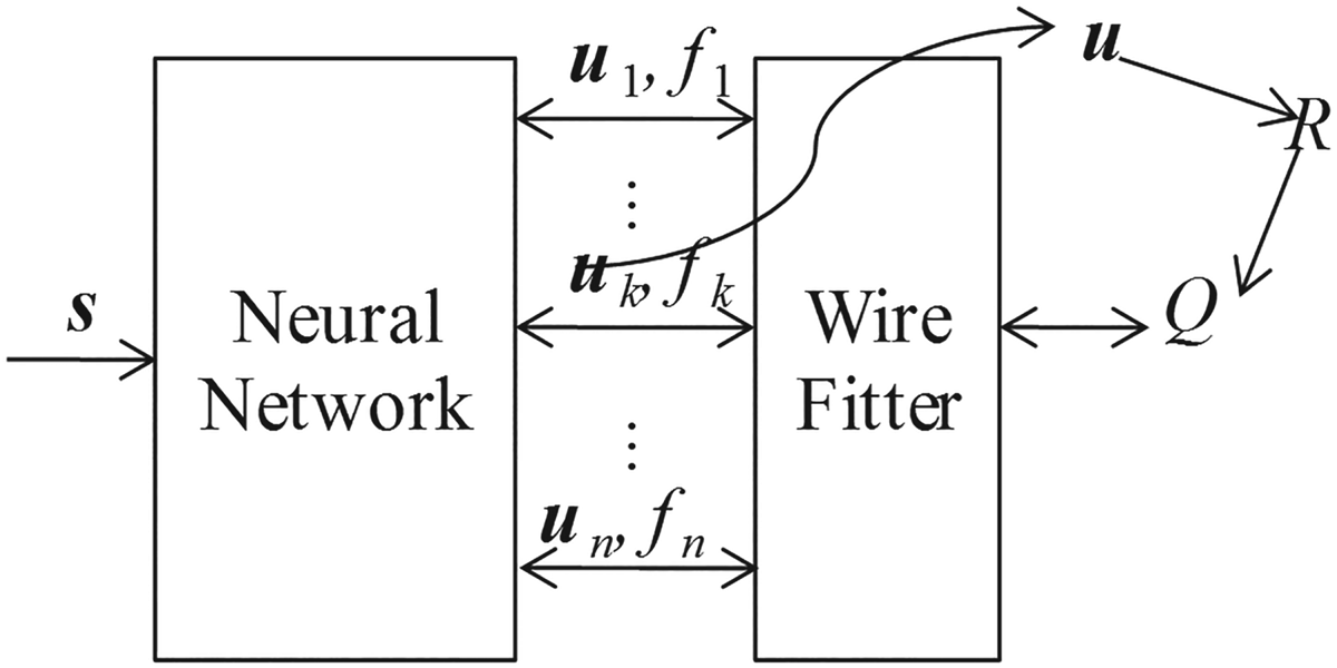
Figure 3. Structure of WFNNQ.
According to the action selection strategy, choose action u k and carry it out. If the neural network has been fully trained, u k may achieve the largest reward. The Q value of the decision u = u k is calculated as the following wire fitting function:
 $$Q( {\textbf{{s}}, \; \textbf{{u}}} ) =\mathop{\mbox{lim}}\limits_{\varepsilon \to 0^+} \frac{\sum_{i=1}^n {\frac{f_i }{\Vert {u-u_i } \Vert ^2+c( {f_{\rm{max}} -f_i } ) +\varepsilon }} }{\sum_{i=1}^n {\frac{1}{\Vert {u-u_i } \Vert ^2+c( {f_{\rm{max}} -f_i } ) +\varepsilon }} }$$
The wire fitting function is a moving least squares interpolator, in which c represents the smoothing factor, and ɛ is a small positive number to avoid the denominator going to infinity.
By the execution of u = u k, the UAV state s transforms to the new state s′, and receives the instantaneous reward R (s, u, s′). Q(s, u) is renewed as:
 $$Q( {\textbf{s}, \; \textbf{u}} ) =( {1-\alpha } ) Q( {\textbf{s}, \; \textbf{u}} ) +\alpha \left[{R( {\textbf{s}, \; \textbf{u}, \; \textbf{s}^{\prime}} ) +\gamma \mathop {\mbox{max}}\limits_{u^{\prime}\in U} Q( {{\textbf{s}}^{\prime}, \; {\textbf{u}}^{\prime}} ) } \right]$$
in which α > 0 is the learning rate, and γ ∈ [0, 1] is the discount factor.
The wire fitting function has a lower computational load as it does not need the inverse operation of the matrix. Furthermore, the interpolation of wire fitting is local, which will not lead to oscillation of the polynomial interpolation. The most outstanding attribute of WFNNQ is that the partial derivative of Q(s, u ) to [u i, f i] T can be easily calculated as
 $$\begin{cases} {\dfrac{\partial Q}{\partial f_i }=\mathop {\mbox{lim}}\limits_{\varepsilon \to 0^+} \frac{( {D_i +cf_i } ) \sum\nolimits_{i=1}^n {D_i^{-1} } -c\sum\nolimits_{i=1}^n {f_i D_i^{-1} } }{\left({D_i \sum\nolimits_{i=1}^n {D_i^{-1} } } \right)^2}} \\ {\dfrac{\partial Q}{\partial u_{ij} }=\mathop{\mbox{lim}}\limits_{\varepsilon \to 0^+} \frac{2( {u_j -u_{ij} } ) \left[{f_i \sum_{i=1}^n {D_i^{-1} } -\sum\nolimits_{i=1}^n {f_i D_i^{-1} } } \right]}{\left({D_i \sum\nolimits_{i=1}^n {D_i^{-1} } } \right)^2}} \end{cases}$$
in which  $D_{i} =u-u_{i} ^{2}+c( {f_{\rm{max}} -f_{i} } ) +\varepsilon $, and u ij is the component of u i. In the 4D trajectory generation problem, u ij (j = 1···3) equals the 3D coupling coefficients k x, k y and k z respectively. These partial derivatives allow the error of the Q(s, u) to be propagated to the neural network.
Uniformly express the partial derivative of Q to z k (f k or u kj) as  $\frac{\partial Q}{\partial z_{k}}=\mathop {\mbox{lim}}\limits_{\Delta \to 0} \frac{\Delta Q}{\Delta z_{k} }$. According to the WFNNQ algorithm (Gaskett et al., Reference Gaskett, Wettergreen and Zelinsky1999
), a scaling factor a(z k
) can be used to share the correction of Δ Q
on pairs of [u i, f i] T
. The variation of z k is
$\frac{\partial Q}{\partial z_{k}}=\mathop {\mbox{lim}}\limits_{\Delta \to 0} \frac{\Delta Q}{\Delta z_{k} }$. According to the WFNNQ algorithm (Gaskett et al., Reference Gaskett, Wettergreen and Zelinsky1999
), a scaling factor a(z k
) can be used to share the correction of Δ Q
on pairs of [u i, f i] T
. The variation of z k is
 $$\Delta z_k =a( {z_k } ) \left({\frac{\partial Q}{\partial z_k }}\right)^{-1}\Delta Q$$
By continually training the neural network, the output Q function will converge to the (u i, y i) with the best reward.
3.2 The reward function
In the distributed multi-UAV system, every vehicle should learn to provide the local optimal trajectory according to its own states and information about its neighbours. The objective of learning is described in the form of the reward function R(s, u, s′). In this paper, the reward function of the i th UAV is designed as:
 $$\begin{align}R_i &=\omega _l L_i +\omega _v \left\| {v_{{\rm max},i} } \right\|^2+\sum\limits_{e_{ij} \in E} {l_{ij} } \int_{t=0}^T {\frac{\omega _d }{p_i \left( t \right)-p_j \left( t \right)^2+\varepsilon }} dt \\ &\quad +\omega _u \sum\limits_{j=1}^N {\mbox{Cu}_{ij} } +\omega _o \sum\limits_{j=1}^{N_{\rm{obs}} } {\mbox{Co}_{ij} }\end{align}$$
where R i is the weighted sum of each trajectory performance including the trajectory length L i, the maximum velocity v max, i, and the reciprocal of the distance between the i th UAV and its neighbours. As the states of the nearer UAVs should be considered preferentially to avoid potential conflicts, l ij in Laplacian matrix L is used to describe the influence of UAVj on the trajectory generation of UAVi.
At the beginning of training, the UAVs may frequently collide with neighbouring UAVs and obstacles. Therefore, the collision penalties Cuij and Coij are added into R i. Cuij is the conflict between UAVi and UAVj, Coij denotes the collision between UAVi and the j th obstacle, and N obs represents the number of obstacles. The notations ωl, ωv, ωd, ωu and ωo are the weights of the performances, p i = [X i, Y i, Z i] T is the position of UAVi.
3.3. The organisation of multi-UAV learning by WoLF-PHC
In the 4D trajectory generation method for multiple UAVs, the learning of the multi-agent system is organised by the WoLF-PHC algorithm. WoLF-PHC uses the mixed strategy π = [πi] n
to select action u, which means that the i th
strategy [u i, f i] T
(i = 1 · · · n
) is selected with the probability πi. There have been some attempts to apply the mixed strategy in continuous state and action spaces, such as the function approximation (Tao and Li, Reference Tao and Li2006), but general methods to design the approximate function are not provided. In this paper, we use the neural network to renew πi and the estimate of average policy  $\bar {\pi }_{i} ( {\textbf{s}, \; \textbf{u}_{i} }) $ in a similar way as WFNNQ. The WFNNQ learning structure with mixed strategy is shown in Figure 4.

Figure 4. Combination of WFNNQ and WoLF-PHC.
At the beginning of learning, WoLF-PHC initialises the mixed strategy of the neural network output as πi = p i(u i, y i) = 1/n . Training then goes on continually to search for the best strategy with the PHC algorithm.
At the first step of iteration, input state s
into the neural network, the output includes [u i, f i] T
, πi and  $\bar{\pi}_{i}\ ( i=1\cdots n) $. After carrying out action u i
according to πi(s, u i
), the probability πi and
$\bar{\pi}_{i}\ ( i=1\cdots n) $. After carrying out action u i
according to πi(s, u i
), the probability πi and  $\bar{\pi}_{i}$ should be corrected.
The correction δi of πi is called the learning rate. To balance the rationality and convergence of learning, WoLF-PHC adopts the WoLF principle to calculate δi, as shown in Equation (14).
 $$\delta _i =\begin{cases} {\delta _{\rm{win}} } & {\mbox{if}\ \sum\limits_{\textbf{u}_i \in U} {\pi_i ( {\textbf{s}, \; \textbf{u}_i } ) Q_i ( {\textbf{s}, \; \textbf{u}_i } ) } >\sum\limits_{\textbf{u}_i \in U} {\bar {\pi }_i ( {\textbf{s}, \; \textbf{u}_i } ) Q_i ( {\textbf{s}, \; \textbf{u}_i } ) } }\\ {\delta _{\rm{lose}} } \hfill & {\mbox{otherwise}} \end{cases}$$
if  $\sum\nolimits_{\textbf{u}_{i} \in U} {\pi _{i} ( {\textbf{s}, \; \textbf{u}_{i} } ) f_{i} ( {\textbf{s}, \; \textbf{u}_{i} } ) } \gt\sum\nolimits_{\textbf{u}_{i} \in U} {\bar {\pi }_{i} ( {\textbf{s}, \; \textbf{u}_{i} } ) f_{i} ( {\textbf{s}, \; \textbf{u}_{i} } ) }$, the strategy u i
is winning, otherwise the strategy is justified as ‘lose’. The algorithm applies δlose > δwin
, and the learning rate decreases with the learning times.
$\sum\nolimits_{\textbf{u}_{i} \in U} {\pi _{i} ( {\textbf{s}, \; \textbf{u}_{i} } ) f_{i} ( {\textbf{s}, \; \textbf{u}_{i} } ) } \gt\sum\nolimits_{\textbf{u}_{i} \in U} {\bar {\pi }_{i} ( {\textbf{s}, \; \textbf{u}_{i} } ) f_{i} ( {\textbf{s}, \; \textbf{u}_{i} } ) }$, the strategy u i
is winning, otherwise the strategy is justified as ‘lose’. The algorithm applies δlose > δwin
, and the learning rate decreases with the learning times.
After the selection of action u i, the correction of the mixed strategy πi is
 $$\pi _i ( {\textbf{s}, \; \textbf{u}_i } ) =\pi _i ( {\textbf{s}, \; \textbf{u}_i } ) + \begin{cases} {\delta _i } & {\mbox{if}\ u_i =u} \\ {\dfrac{-\delta _i }{\vert U\vert -1}} & {\mbox{otherwise}} \end{cases}$$
in which u is the selected action.
The average strategy is then renewed as
 $$\bar {\pi }_i ( {\textbf{s}, \; \textbf{u}_i } ) =\bar {\pi }_i ( {\textbf{s}, \; \textbf{u}_i } ) +\beta \frac{\pi _i ( {\textbf{s}, \; \textbf{u}_i } ) -\bar {\pi }_i ( {\textbf{s}, \; \textbf{u}_i } ) }{n_l }$$
in which n l is the number of iterations, and β is the discount factor.
The neural network is then trained with the state s and the output actions  $a_{i} =[ u_{i}, \; f_{i}, \; \pi_{i}, \; \bar{\pi}_{i}] ^{{\rm T}}\ ( i=1\cdots n) $. By continual correction of πi, the best rewarded strategy will achieve the highest decision probability. The 4D trajectory generation method based on multi-agent WFNNQ learning is summed up in Figure 5.
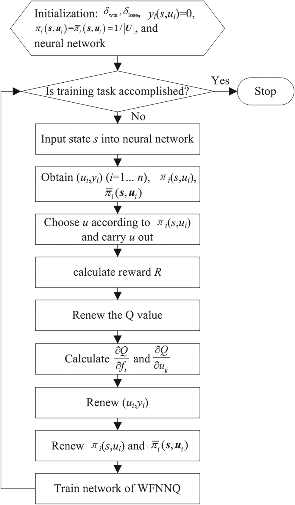
Figure 5. 4D-trajectory generation based on MAQL.
4. SIMULATIONS AND RESULTS
The simulations carried out to validate the performance of the proposed 4D trajectory generation method based on the I-tau-G strategy and MAQL (tau-MAQL) are summarised in this section. For comparison, the tests are handled by the 4D trajectory generation method based on the I-tau-G strategy and decentralised receding horizontal optimisation (I-tau-GDRHO) (Yang et al., Reference Yang, Fang and Li2016).
A realistic multi-UAV cooperation simulation scenario is designed as there is no benchmark to verify the validity of the 4D trajectory generation method for multiple UAVs (Alejo et al., Reference Alejo, Cobano, Heredia and Ollero2013 ). In this scenario, five homogeneous UAVs complete a typical cooperative formation aggregation mission in a virtual 3D space of 25 × 25 × 25 m3 . UAVs should generate collision-free trajectories and simultaneously approach the aggression position with the desired speed at the arrival time. For each UAV, the maximum velocity was set to v max = 6 m/s, the distance measurement range R avoid = 15 m, the safe separation R safe = 1 m, and the valid communication distance R c = 20 m. The initial and goal motion states of UAVs are randomly generated for each test case, and the arrival time for the formation aggregation mission is T = 20 s. All of the simulations were performed on a laptop with a 2·6 GHz Core i5-3230M CPU and 4 GB of RAM running Matlab R2015a.
4.1. Simulations of 4D trajectory generation capability
To validate the 4D trajectory generation capability of the proposed tau-MAQL method, 100 test cases were randomly generated. The proposed method is trained by the cases one by one until the reward function of reinforcement learning approaches convergence. Each of the cases was trained for 200 episodes.
Figure 6 shows the mean cost of the 4D trajectories in the first (Figure 6(a)) and fifth (Figure 6(b)) cases, in which the cost is the reward of movement along a trajectory, as shown in Equation (13). In Figure 6(a), along with the training steps, the total trajectory cost of the multi-UAV system descends and converges. After the training of five cases, as shown in Figure 6(b), the standard deviation in the 200 episodes is less than 10% of the average cost. Therefore, it can be concluded that the tau-MAQL method converged. The other 95 cases are used to test the adaptive capability of tau-MAQL to similar missions and environments.

Figure 6. Mean cost of 4D trajectories for five UAVs: (a) first case, (b) fifth case.
4.2. Simulations of adaptive capability to similar tasks
The trained tau-MAQL method was used to solve the other 95 test cases. The statistical data of the performance is shown in Table 1. The notation  $\bar{t}$ is the mean decision time for different numbers of communication-established UAVs. Because tau-MAQL does not need to optimise the problem repeatedly, its decision time
  $\bar{t}$ is obviously smaller than that of I-tau-GDRHO for different UAV numbers.
  $\bar{C}_{r} =\bar{R}_{{\rm MAQL}}/\bar{R}_{{\rm DRHO}}$ refers to the mean cost ratio between trajectories generated by tau-MAQL and I-tau-GDRHO, in which
  $\bar{R}_{{\rm MAQL}}$ and
  $\bar{R}_{{\rm DRHO}}$ denote the motion cost for a UAV to move along the trajectory provided by individual methods. The calculation of the trajectory cost is the same as the reward function shown in Equation (13). On average, the motion cost of trajectories generated by tau-MAQL is 64·6% larger than the comparison method with receding optimisation. Hence the proposed tau-MAQL can generate near optimal 4D trajectories with less time consumption than I-tau-GDRHO.
Table 1. Performance comparison of generation of 4D trajectories.

The flight security of trajectories is compared in Table 2. The notations Ncu, Nco and Ncb denote the number of cases in which the trajectories conflict with only UAVs, only obstacles, and both UAVs and obstacles, respectively. A total of 95 test cases were carried out, four of which encountered collision problems using the tau-MAQL method. Though the flight security of I-tau-GDRHO is better, tau-MAQL plans trajectory directly with learning experience, but without complicated optimisation time and again. Therefore, the proposed tau-MAQL method can generate near optimal 4D trajectories with less time consumption, and can guarantee flight safety for similar but untrained cases. Furthermore, flight safety will be gradually improved by training for more cases.
Table 2. Number of cases with conflicts.

4.3. Simulations of 4D trajectory tracking
To examine the flyability and tracking error tolerance of the generated 4D trajectories, the kinematics and dynamics model of five quad-rotor UAVs was designed in Simulink. To visualise the simulated results, a 3D scenario was designed by the Virtual and Reality Toolbox of Matlab, as shown in Figure 7. A video of this simulation is shown in the attachment to this paper.

Figure 7. Visualised 3D simulation scenario.
Figure 8 shows the spatial tracking results of the 4D trajectories planned by tau-MAQL. The arbitrarily generated initial positions are marked by hovering UAVs from UAV1 to UAV5, the destinations are numbered from G1 to G5, and the obstacles are described by spheres.

Figure 8. Spatial tracking results of 4D trajectories.
As not all the details of the flights can be displayed in this part, the most dangerous trajectory, namely the trajectory of the UAV, is chosen to show the tracking results. The closest distances between each UAV and other UAVs are shown in Figure 9, and the distances between each UAV and the nearest obstacles are shown in Figure 10. The dashed bold line represents the warning separation of 1 m. According to Figures 9 and 10, the UAVs keep a safe distance from each other and a safe distance from obstacles, so the flight safety of all UAVs is guaranteed.

Figure 9. Closest distance of each UAV from another UAV.

Figure 10. Distance between each UAV and the nearest obstacles.
Figure 11 shows the 3D tracking results of UAV4. The 4D trajectory provides smooth guidance for movements along three axes, and the UAV arrives at its destination at the prescribed arrival time. The velocities of the five UAVs during trajectory tracking are shown in Figure 12, showing that the 4D guidance is able to fulfil the dynamic constraints of the UAVs, as the trajectories rapidly become smooth.

Figure 11. 3D positions of UAV4.

Figure 12. Velocity of UAVs.
5. REAL-TIME FLIGHT SIMULATION FOR SUBSONIC UAVS
In order to evaluate sufficiently the performance of 4D trajectory generation using tau-MAQL for high-speed fixed-wing UAVs, a real-time flight simulation based on our high subsonic UAVs was carried out, using an aerodynamic model of the UAVs. In the simulation. three UAVs took off from the same airport at different times (at 30 s intervals), and performed a formation flight task that involved assembly at the desired time, a triangle shaped formation flight, and then separation from each other. Figure 13 shows the tracking results of the 4D trajectories planned by tau-MAQL. Tau-MAQL provided a circuitous route for UAV1, which took off first, and planned a shortcut for UAV3 to save time. The result manifested that the three aircraft finally arrived at the rally point close to the desired time, and the errors were kept within 3·2 s.

Figure 13. Tracking results of 4D trajectories of three UAVs.
Relative distances from the second UAV in 3D, and the forward components, are shown in Figures 14 and 15, respectively. Figure 16 shows lateral distances from the planned trajectory of the second UAV. When the UAVs arrived at the rally point, they continued flying side by side with 500 m lateral separation from their neighbours as designed, and their relative velocities were close to zero, as shown in Figures 17 and 18. The flight formation then transformed into the ‘Δ’ and ‘∇’ forms successively, as planned by tau-MAQL. The UAVs arrived at their own destinations simultaneously, with the same desired velocity (170 m/s). The UAVs then separated and flew away from each other in a lateral direction with the desired relative velocities and finally returned to the airport.

Figure 14. 3D relative distances of UAV1 and UAV3 from UAV2.

Figure 15. Forward distances of UAV1 and UAV3 from UAV2.

Figure 16. Lateral distances of UAV1 and UAV3 from the planned trajectory of UAV2.

Figure 17. Forward velocities of UAV1 and UAV3 relative to UAV2.

Figure 18. Lateral velocities of UAV1 and UAV3 relative to UAV2.
Although there were no other obstacles in the air, except for neighbour UAVs, the position errors shown in Figures 14–16, and the relative velocities shown in Figures 17 and 18, demonstrate that the 4D trajectories planned by tau-MAQL were safe and flyable for our UAVs, which were capable of 4D guidance.
6. CONCLUSION
In this paper, a multi-UAV 4D trajectory generation method (tau-MAQL) based on the I-tau-G guidance strategy and MAQL is presented. The 4D trajectories generated by the improved tau-G strategy were found to guide both position and velocity to the desired values at the desired time. As it is not appropriate to discretise the states and actions of the trajectories provided by the I-tau-G strategy, WFNNQ learning was adopted. The WoLF-PHC algorithm was also applied to organise the multi-UAV system.
The main advantage of this method is the combination of bionic tau theory and reinforcement learning in multi-UAV applications. With the benefit of the I-tau-G strategy, the 4D trajectory can guide the UAV movements smoothly with desired initial and terminal velocities. Furthermore, the trained MAQL can obviously improve the planning efficiency better than optimisation methods.
Challenging dynamic simulations of multi-UAV formations were carried out to validate the convergence, execution time, adaptive capability and trajectory quality of the proposed tau-MAQL method. The simulation results show that tau-MAQL can provide near optimal 4D trajectories with conspicuously greater efficiency in terms of computing time. The flight safety, flyability and 4D guidance capability of the trajectories can meet the requirements for cooperative flight. Meanwhile, the trained tau-MAQL was found to have enough adaptive capability to deal with similar environments and missions.
ACKNOWLEDGEMENTS
This work was jointly funded by the National Natural Science Foundation of China (Nos. 61703366), and the Fundamental Research Funds for the Central Universities (No. 2016| FZA4023, 2017QN81006).


