


1. INTRODUCTION
The Inertial Navigation System (INS) achieves high precision navigation through continuous integral computation based on angular velocity and acceleration, and is an essential component of a long-range missile (Chang et al., Reference Chang, Hu and Li2015; Cheng and Li, Reference Cheng and Li2013; Liu et al., Reference Liu, Xu and Liu2015; Lu et al., Reference Lu, Xie and Chen2009). The initial alignment is one of the key technologies of a missile-borne INS. Its rapidity and precision are the two most important parameters which determine the launching preparation time and the navigation precision of the missile, respectively (Wang et al., Reference Wang, Sun and Zhang2012).
Normally, the initial alignment process is divided into two phases, coarse and fine alignment. The purpose of coarse alignment is to provide a desirable initial condition for the fine alignment (Li et al., Reference Li, Fang and Du2012; Chang et al., Reference Chang, Li and Chen2015; Wu et al., Reference Wu, Wu and Hu2010). Some fine initial alignment methods have been investigated in the last few decades. These methods are mainly performed on a stationary base after the missile has been erected along the X-axis from the horizontal state to the vertical state with the pitch angle varying by 90° (Lu et al., Reference Lu, Xie and Li2016; Li et al., Reference Li, Wang and Lv2015). For instance, the most common optical alignment method adopts some optical instruments to obtain the initial attitude angle, which is the Euler angle of the INS. However, the optical alignment method is complex and time consuming, and cannot meet the requirement of rapidity (Li et al., Reference Li, Wang and Lv2015). Usually, a fine self-alignment method using a Kalman filter is adopted (Wu et al., Reference Wu, Wang and Zhu2014). It is performed on a stationary base after the missile has been erected to the vertical state. The extra time is devoted to the fine self-alignment method, and some unobservable state variables are difficult to accurately estimate quickly (Gao et al., Reference Gao, Zhang and Wang2015; Wu et al., Reference Wu, Zhang and Wu2012). Therefore, the rapidity of fine initial alignment will be severely influenced (Cho et al., Reference Cho, Lee and Wang2013; Wu et al., Reference Wu, Wu and Hu2011). How to improve the rapidity of fine initial alignment has become an urgent problem for missile-borne INS development.
In order to solve the aforementioned problem, a fast fine initial self-alignment method for a missile-borne INS is proposed, which is performed during the erecting process on a stationary base. According to the proposed convected Euler angle error model, the erecting manoeuvre can be optimised to prevent the large Euler angle errors. The fine initial alignment model is established to estimate and correct the initial misalignment. The observability degree analysis indicates that the system observability can be improved. The proposed method may not only share the erecting manoeuvre, but also improve the system observability so that the alignment time can be reduced. Several experiments have been carried out, and verify that the proposed method is effective for improving the rapidity of the fine initial alignment for a missile-borne INS.
This paper is organised as follows. In Section 2, the convected Euler angle error is modelled to optimise the erecting manoeuvre. Section 3 presents the fine initial alignment model. The observability degree is analysed in Section 4. Section 5 introduces the fine alignment experiment and finally, conclusions are drawn in Section 6.
2. MODELLING CONVECTED EULER ANGLE ERROR TO OPTIMISE ERECTING MANOEUVER
For the INS, the digital computational platform is theoretically equivalent to the local level navigation frame. Gyroscope outputs are used to maintain the digital computational platform. Accelerometer outputs are obtained and then integrated to acquire velocity and position. It is vital to determine the body attitude matrix, which represents a coordinate system transformation relation of the body frame with respect to the navigation frame.
The angular velocity from the body frame to the navigation frame is denoted in the body frame, which can be calculated by:
 $$\omega_{nb}^{b}=\omega_{ib}^{b}-C_{n}^{b}\omega_{in}^{n}=\omega_{ib}^{b}-C_{n}^{b}(\omega_{ie}^{n}+\omega_{en}^{n})$$
where  $\omega_{ib}^{b}$ is an angular velocity vector of the body frame with respect to the inertial frame denoted in the body frame, and can be directly measured by gyroscopes.
  $\omega_{in}^{n}$ is the angular velocity vector of the navigation frame with respect to the inertial frame denoted in the navigation frame, which can be written as:
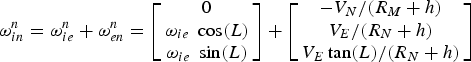 $$\omega_{in}^{n}=\omega_{ie}^{n}+\omega_{en}^{n}=\left[\matrix{ 0 \cr \omega_{ie}\ \cos(L) \cr \omega_{ie}\ \sin(L) }\right] +\left[\matrix{ -V_{N}/(R_{M} +h) \cr V_{E}/(R_{N} +h) \cr V_{E}\tan(L)/(R_{N} +h) }\right]$$
where  $\omega_{ie}^{n}$ is the angular velocity vector of the Earth frame with respect to the inertial frame denoted in the navigation frame.
  $\omega_{en}^{n}$ is the angular velocity vector of the navigation frame with respect to the Earth frame denoted in the navigation frame. V E and V N are the velocity in east and north directions. R M and R N are the transverse and meridian radii of curvature. L and h represent latitude and height respectively.
As shown in Figure 1, to accurately derive the Euler angle error differential equation, the transformation relation between the angular velocity of the body frame with respect to the navigation frame denoted in the body frame and the Euler angle velocities, can be expressed as:
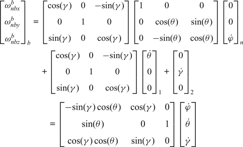 $$\eqalign{ \left[\matrix{ \omega_{nbx}^{b} \cr \omega_{nby}^{b} \cr \omega_{nbz}^{b} }\right]_b =&\left[\matrix{ \cos(\gamma) & 0 & -\!\sin(\gamma) \cr 0 & 1 & 0 \cr \sin(\gamma) & 0 & \cos(\gamma) }\right]\left[\matrix{ 1 & 0 & 0 \cr 0 & \cos(\theta) &\sin(\theta) \cr 0 & -\!\sin(\theta) &\cos(\theta) }\right]\left[\matrix{ 0 \cr 0 \cr \dot{\varphi} }\right]_n \cr +&\left[\matrix{ \cos(\gamma) & 0 & -\!\sin(\gamma) \cr 0 & 1 & 0 \cr \sin(\gamma) & 0 & \cos(\gamma) }\right]\left[\matrix{ \dot{\theta} \cr 0 \cr 0 }\right]_1+\left[\matrix{ 0 \cr \dot{\gamma} \cr 0 }\right]_2 \cr &=\left[\matrix{ -\!\sin(\gamma)\cos(\theta) & \cos(\gamma) & 0 \cr \sin(\theta) & 0 & 1 \cr \cos(\gamma)\cos(\theta) &\sin(\gamma) & 0 }\right]\left[\matrix{ \dot{\varphi} \cr \dot{\theta} \cr \dot{\gamma} }\right]}$$
where  $\omega_{nbi}^{b}$ is the angular velocity of the body frame with respect to the navigation frame denoted in body frame along the i axis. The Euler angle differential equation induced by the angular velocities of the body frame with respect to the navigation frame denoted in the body frame can be written as:
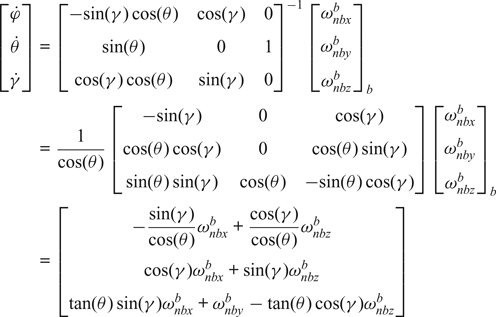 $$\eqalign{ \left[\matrix{ \dot{\varphi} \cr \dot{\theta} \cr \dot{\gamma} }\right] &=\left[\matrix{ -\!\sin(\gamma)\cos(\theta) &\cos(\gamma) & 0 \cr \sin(\theta) & 0 & 1 \cr \cos(\gamma)\cos(\theta) &\sin(\gamma) & 0 }\right]^{-1} \left[\matrix{ \omega_{nbx}^{b} \cr \omega_{nby}^{b} \cr \omega_{nbz}^{b} }\right]_b \cr &={1 \over \cos(\theta)}\left[\matrix{ -\!\sin(\gamma) & 0 & \cos(\gamma) \cr \cos(\theta)\cos(\gamma) & 0 & \cos(\theta)\sin(\gamma) \cr \sin(\theta)\sin(\gamma) & \cos(\theta) & -\!\sin(\theta)\cos(\gamma) }\right]\left[\matrix{ \omega_{nbx}^{b} \cr \omega_{nby}^{b} \cr \omega_{nbz}^{b} }\right]_b \cr &=\left[\matrix{ -{\sin(\gamma) \over \cos(\theta)}\omega_{nbx}^{b} +{\cos(\gamma) \over \cos(\theta)}\omega_{nbz}^{b} \cr \cos(\gamma)\omega_{nbx}^{b}+\sin(\gamma)\omega_{nbz}^{b} \cr \tan (\theta)\sin(\gamma)\omega_{nbx}^{b}+\omega_{nby}^{b} -\tan (\theta)\cos(\gamma)\omega_{nbz}^{b} }\right]}$$
The differentiation errors of the Euler angle between the azimuth φc, pitch θc, roll γc with respect to the computational frame ocxcyczc and azimuth φ, pitch θ and roll γ with respect to the navigation frame onxnynzn, can be expressed as:
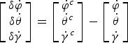 $$\left[\matrix{ \delta\dot{\varphi} \cr \delta\dot{\theta} \cr \delta\dot{\gamma} }\right]=\left[\matrix{ \dot{\varphi}^c \cr \dot{\theta}^c \cr \dot{\gamma}^c }\right] -\left[\matrix{ \dot{\varphi} \cr \dot{\theta} \cr \dot{\gamma} }\right]$$
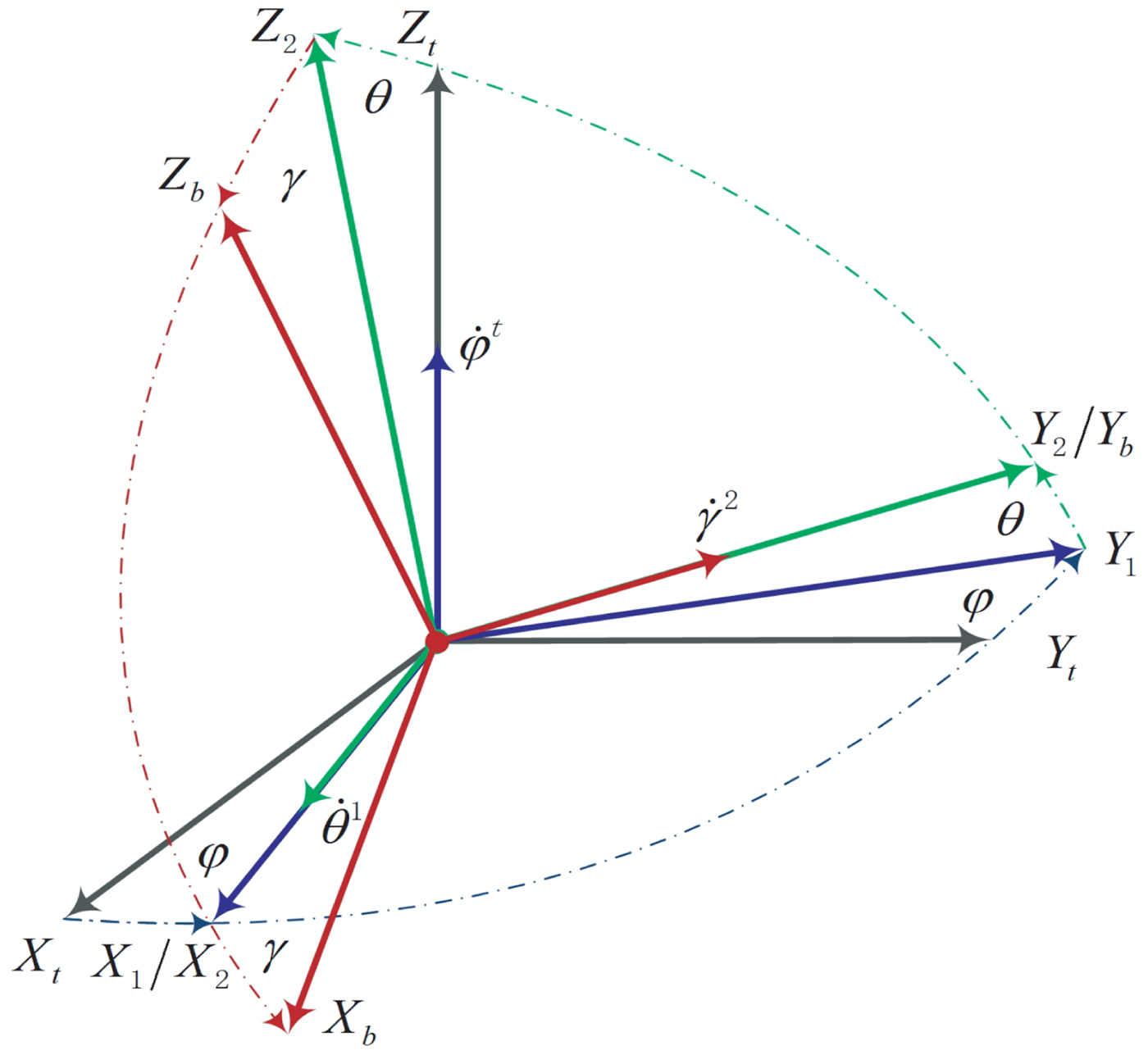
Figure 1. Euler angles transformation relation for INS.
Using Equations (4) and (5), the differential equations of Euler angle error in azimuth, pitch and roll can be obtained. The differential equation of pitch angle error is written as:
 $$\delta\dot{\theta}=\dot{\theta}^{c}-\dot{\theta}=\cos(\gamma^{c})\omega_{nbx}^{b}+\sin(\gamma^{c})\omega_{nbz}^{b}-\big[\cos(\gamma^{c}-\delta\gamma)\omega_{nbx}^{b}+\sin(\gamma^{c}-\delta\gamma)\omega_{nbz}^{b}\big]$$
 By Taylor expansion, we have  $\sin(\delta\gamma)\approx\delta\gamma, \cos(\delta \gamma)\approx 1$; ignoring the terms as small as the second order, the differential equation of pitch error can be rewritten as:
 $$\delta\dot{\theta}\approx\big[\cos(\gamma^{c})\omega_{nbz}^{b}-\!\sin(\gamma^{c})\omega_{nbx}^{b}\big]\delta\gamma$$
The differential equation of roll angle error can be obtained as:
 $$\eqalign{ \delta\dot{\gamma}=&\dot{\gamma}^{c}-\dot{\gamma}=\tan(\theta^{c})\big[\sin(\gamma^{c})\omega_{nbx}^{b}-\!\cos(\gamma^{c})\omega_{nbz}^{b}\big]+\omega_{nby}^{b} \cr &-\tan(\theta^{c}-\delta\theta)\big[\sin(\gamma^{c}-\delta\gamma)\omega_{nbx}^{b}-\!\cos(\gamma^{c}-\delta\gamma)\omega_{nbz}^{b}\big]-\omega_{nby}^{b}}$$
 Based on Taylor expansion, we have  $\sin(\delta\theta)\approx\delta\theta$,
  $\tan(\theta^{c}-\delta\theta)=\tan(\theta^{c})-\sec^{2}(\theta^{c})\delta\theta$; ignoring the terms as small as the second order, the differential equation of the roll angle error can be rewritten as:
 $$\delta\dot{\gamma}=\tan(\theta^{c})\big[\cos(\gamma^{c})\omega_{nbx}^{b}+\sin(\gamma^{c})\omega_{nbz}^{b}\big]\delta\gamma+\sec^{2}(\theta^{c})\big[\sin(\gamma^{c})\omega_{nbx}^{b}-\!\cos(\gamma^{c})\omega_{nbz}^{b}\big]\delta\theta$$
The differential equation of azimuth angle error can be written as:
 $$\eqalign{ \delta\dot{\varphi}=\dot{\varphi}^{c}-\dot{\varphi}&=-{1 \over \cos(\theta^{c})}\big[\sin(\gamma^{c})\omega_{nbx}^{b}-\!\cos(\gamma^{c})\omega_{nbz}^{b}\big] \cr &\quad +{1 \over \cos(\theta^{c}-\delta\theta)}\big[\sin(\gamma^{c}-\delta\gamma)\omega_{nbx}^{b}-\!\cos(\gamma^{c}-\delta\gamma)\omega_{nbz}^{b}\big] }$$
 Based on Taylor expansion, assuming  $\sin(\delta\theta)\approx\delta\theta$,
  $\sin(\delta\gamma)\approx\delta\gamma$,
  $\cos(\delta\theta)\approx\cos\break (\delta\gamma)\approx 1$,
  $\sec(\theta^{c}-\delta\theta)\approx\sec(\theta^{c})-\sec(\theta^{c})\tan(\theta^{c})\delta\theta$, ignoring the terms as small as the second order, the differential equation of azimuth angle error can be rewritten as:
 $$\delta\dot{\varphi}\approx\sec(\theta^{c}) \left\{\matrix{ \big[\cos(\gamma^c)\omega_{nbz}^{b} -\!\sin(\gamma^{c})\omega_{nbx}^{b}\big]\tan (\theta^{c})\delta\theta \cr -\big[\cos(\gamma^{c})\omega_{nbx}^{b} +\sin(\gamma^{c})\omega_{nbz}^{b}\big]\delta\gamma }\right\}$$
According to Equations (7), (9) and (11), the differential equation of convected Euler angle error caused by the erecting manoeuvre can be obtained as:
 $$\eqalign{ \left[\matrix{ \delta\dot{\theta} \cr \delta\dot{\gamma} \cr \delta\dot{\varphi} }\right] ={1 \over \cos (\theta^{c})} &\left[\matrix{ 0 \cr \sec(\theta^{c})\big(\sin(\gamma^{c})\omega_{nbx}^{b}-\!\cos(\gamma^{c})\omega_{nbz}^{b}\big) \cr \sec(\theta^c)\sin(\theta^{c})\big(-\!\sin(\gamma^{c})\omega_{nbx}^{b}+\cos(\gamma^{c})\omega_{nbz}^{b}\big) }\right. \cr & \quad \left.\matrix{ -\!\cos(\theta^{c})\sin(\gamma^{c})\omega_{nbx}^{b}+\cos(\theta^{c})\cos(\gamma^{c})\omega_{nbz}^{b} & 0 \cr \sin(\theta^{c})\cos(\gamma^{c})\omega_{nbx}^{b}+\sin(\theta^{c})\sin(\gamma^{c})\omega_{nbz}^{b} & 0 \cr -\!\cos(\gamma^{c})\omega_{nbx}^{b}-\!\sin(\gamma^{c})\omega_{nbz}^{b} & 0 }\right] \left[\matrix{ \delta\theta \cr \delta\gamma \cr \delta\varphi }\right]}$$
The convected Euler angle error equation can be obtained as:
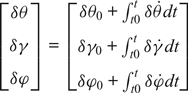 $$\left[\matrix{ \delta\theta \cr \delta\gamma \cr \delta\varphi }\right]=\left[\matrix{ \delta\theta_{0}+\int_{t0}^{t}\delta\dot{\theta} dt \cr \delta\gamma_{0}+\int_{t0}^{t}\delta\dot{\gamma} dt \cr \delta\varphi_{0}+\int_{t0}^{t}\delta\dot{\varphi} dt }\right]$$
where δφ0, δθ0, δγ0 are errors of initial azimuth, pitch and roll of INS calculated by analytical coarse alignment, respectively. The convected Euler angle error equation is related to the motion of the missile-borne INS and aimed to optimise the erecting manoeuvre. It is distinct from the traditional error equation of INS which is the misalignment angle error equation and is applied to analyse the error of INS in navigation computation.
In the normal erecting manoeuvre, the missile body is rotated 90° along the X-axis from the horizontal state to the vertical state. From Equations (12) and (13), it can be found that the convected Euler angle errors will gradually increase with the pitch angle. Moreover, the convected Euler angle errors of a missile-borne INS can be affected by the angular velocities of the body frame with respect to the navigation frame denoted in the body frame along X-and Z-axes  $\omega_{nbx}^{b}$,
  $\omega_{nbz}^{b}$, except Y-axis
  $\omega_{nby}^{b}$. Therefore, the missile-borne INS should be erected from horizontal to the vertical state along the Y-axis instead of the X-axis. The optimised erecting manoeuvre can prevent the larger Euler angle errors, and can be shared with the fine initial alignment. In this way, the rapidity of the fine initial alignment can be improved.
3. FINE INITIAL ALIGNMENT MODEL
3.2. State equation modelling of the fine initial alignment
A Kalman filter is designed to estimate and correct the initial misalignment in real-time. According to the error equation of INS, the state equation of system is expressed by:
 $$\dot{\bi X}={\bi FX}+{\bi GW}$$
where X is the state vector of Kalman filter, that is a fifteen-dimensional state variable.  ${\bi X}=[\phi_{{\rm E}} \quad \phi_{{\rm N}} \quad \phi_{{\rm U}} \quad \delta V_{{\rm E}} \quad \delta V_{{\rm N}} \quad \delta V_{{\rm U}} \quad \delta L \quad \delta\lambda \quad \delta h \quad \varepsilon_{E} \quad \varepsilon_{N} \quad \varepsilon_{U} \quad \nabla_{E} \quad \nabla_{N} \quad \nabla_{U}]^{T}$ where
  $\phi_{i},\ \delta V_{i},\ \varepsilon_{i}$ and ∇i are misalignment, velocity error, gyroscope drift and accelerometer bias along the i axis in the navigation frame and
  $\delta L,\ \delta\lambda$ and δ h are the errors of latitude, longitude and altitude. W is system noise,
  ${\bi W}=[\matrix{ w_{\varepsilon_{E}} &w_{\varepsilon_{N}} &w_{\varepsilon_{U}} &w_{\nabla_{E}} &w_{\nabla_{N}} &w_{\nabla_{U}}}]^{T}$ which includes gyroscope random errors and accelerometer random errors. F is a 15 × 15 dimensional state transformation matrix, and can be expressed as:
 $${\bi F}=\left[\matrix{ F_{1} & F_{2} & F_{3} & C_{b}^{n} & 0_{3\times 3} \cr F_{4} & F_{5} & F_{6} & 0_{3\times 3} & C_{b}^{n} \cr 0_{3\times 3} & F_{7} & F_{8} & 0_{3\times 3} & 0_{3\times 3} \cr 0_{3\times 3} & 0_{3\times 3} & 0_{3\times 3} & 0_{3\times 3} & 0_{3\times 3} \cr 0_{3\times 3} & 0_{3\times 3} & 0_{3\times 3} & 0_{3\times 3} & 0_{3\times 3} }\right]$$
where every submatrix F i is described (Han and Fang, Reference Han and Fang2013). G is a 15×6 dimensional process noise matrix, and can be expressed as:
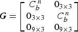 $${\bi G}= \left[\matrix{ C^{\,n}_b &0_{3\times 3} \cr 0_{3\times 3} & C^{\,n}_b \cr 0_{9\times 3} &0_{9\times 3} }\right]$$
where  $C_{b}^{\,n}$ is an attitude transformation matrix from the body frame to the navigation frame.
3.2. Measurement and measurement equation modelling of the fine initial alignment
The missile launching system includes the launching vehicle, missile with INS, and erecting mechanism as shown in Figure 2. The position of the launching location can be obtained through the Global Navigation Satellite System (GNSS) receiver of the launching vehicle. After coarse alignment, the missile will be erected from the horizontal to the vertical state. Since the launching vehicle is static, the measurements including positions and velocities can be calculated by modelling the lever arm. The lever arm  ${\bf R}_{I}^{b}=[X_{I}\ Y_{I}\ Z_{I}]^{T}$, refers to the spatial vector between the rotating centre of erecting mechanism O o and the sensing centre of the missile-borne INS O b in the body frame ObXbYbZb. The positions and velocities of the missile-borne INS sensing centre O b relative to erecting mechanism rotating centre O o are time-varying.
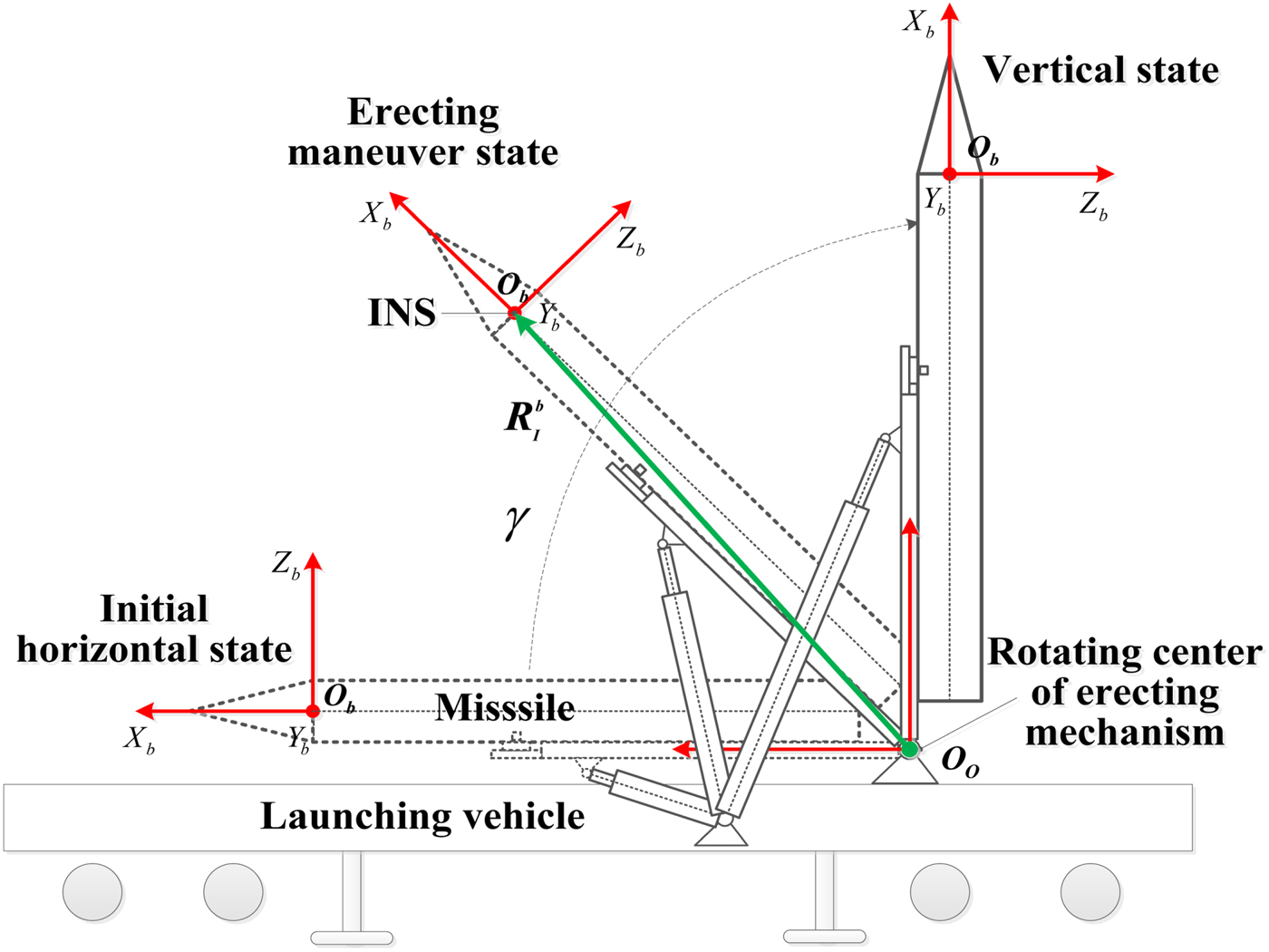
Figure 2. The missile launching system mainly include launching vehicle, missile with INS and erection mechanism.
The missile can be erected from the horizontal to the vertical state as shown in Figure 2. The position measurement of the missile-borne INS centre can be calculated by modelling of the lever arm. Compared with the rotating centre of the erecting mechanism O o, the relative position vector calculated by the lever arm can be expressed as:
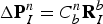 $$\Delta {\bf P}_{I}^{n}=C_{b}^{n}{\bf R}_{I}^{b}$$
Using the lever arm model, the position measurement vector in the sensing centre of the missile-borne INS can be calculated in real-time:
 $${\bf P}_{S}^{n}={\bf P}_{O}^{n}+{\bf \Pi}\triangle {\bf P}_{I}^{n}={\bf P}_{O}^{n}+{\bf \Pi} C_{b}^{n}{\bf R}_{I}^{b}$$
where  ${\bf P}_{O}^{n}$ represents the position vector in the rotating centre of the erecting mechanism O o in the navigation frame,
  ${\bf P}_{O}^{n}=[L_{o}\ \lambda_{o}\ h_{o}]^{T}$. Π represents a matrix which can transform a position vector from the navigation frame to the Earth frame. The position measurement of fine alignment in the erecting process can be further expressed as:
 $$\left[\matrix{ L_{s} \cr \lambda_{s} \cr h_{s} }\right]=\left[\matrix{ L_{o} \cr \lambda_{o} \cr h_{o} }\right]+ \left[ \matrix{ {1 \over R_{M}+h} &0 &0 \cr 0 &{\sec L \over R_{N}+h} &0 \cr 0&0 &1} \right] \left[\matrix{ T_{11} & T_{21} & T_{31} \cr T_{12} & T_{22} & T_{32} \cr T_{13} & T_{23} & T_{33} }\right]\left[\matrix{ X_{I} \cr Y_{I} \cr Z_{I} }\right]$$
where T ij is an element of attitude transformation matrix  $C_{b}^{\,n}$ with i, j = 1, 2, 3.
When the launching vehicle stops at the launching location, the velocity of the rotating centre of the erecting mechanism,  ${\bf V}_{O}^{n}$ can be assumed as
  ${\bf V}_{O}^{n}=[\matrix{ 0 &0 &0}]^{T}$. The velocity measurement in the sensing centre of the missile-borne INS can be calculated in real-time:
 $${\bf V}_{S}^{n}={\bf V}_{O}^{n}+\triangle {\bf V}_{I}^{n}={\bf V}_{O}^{n}+C_{b}^{n}(\omega_{nb}^{b}\times {\bf R}_{I}^{b})=C_{b}^{n}(\omega_{nb}^{b}\times {\bf R}_{I}^{b})$$
where  $\omega_{nb}^{b}$ is an angular velocity vector of the missile-borne INS body frame with respect to the navigation frame denoted in the missile-borne INS body frame, and has been given in Equation (1). The angular velocity vector
  $\omega_{nb}^{b}$ can be further expressed as:
 $$\left[\matrix{ \omega_{nbx}^{b} \cr \omega_{nby}^{b} \cr \omega_{nbz}^{b} }\right]=\left[\matrix{ \omega_{ibx}^{b} \cr \omega_{iby}^{b} \cr \omega_{ibz}^{b} }\right] -\left[\matrix{ T_{11} & T_{12} & T_{13} \cr T_{21} & T_{22} & T_{23} \cr T_{31} & T_{32} & T_{33} }\right]\left[\matrix{ -{V_{N} \over R_{M}+h} \cr \omega_{ie} \cos L+{V_{E} \over R_{N}+h} \cr \omega_{ie} \sin L+{V_{E}\tan L \over R_{N}+h} }\right]$$
where VE, VN, VU are the velocities in east, north and up directions, which can be updated in real-time by fine alignment.  $R_{M}=R_{0}(1-e^{2})/(1-e^{2}\sin^{2}L)^{3/2}, R_{N}=R_{0}/(1-e^{2}\sin^{2}L)^{1/2}$ with R 0 is the radius of the Earth. e is the flat ratio of the navigation system. ωie is the Earth angular rate. The velocity measurement of the missile-borne INS sensing centre can be further expressed as:
 $$\left[\matrix{ V_{SE}^{n} \cr V_{SN}^{n} \cr V_{SU}^{n} }\right]=\left[\matrix{ T_{11} & T_{21} & T_{31} \cr T_{12} & T_{22} & T_{32} \cr T_{13} & T_{23} & T_{33} }\right] \left(\left[\matrix{ 0 & -\omega_{nbz}^{b} & \omega_{nby}^{b} \cr \omega_{nbz}^{b} & 0 & -\omega_{nbx}^{b} \cr -\omega_{nby}^{b} & \omega_{nbx}^{b} & 0 }\right]\left[\matrix{ X_{I} \cr Y_{I} \cr Z_{I} }\right]\right)$$
where  $V_{SE}^{n},\ V_{SN}^{n}$ and
  $V_{SU}^{n}$ are the velocity measurements of the fine initial alignment along east, north and up directions respectively. These measurements can be obtained by the modelling of the lever arm, which are independent of external equipment, ensuring the accuracy of measurement for fine alignment.
Taking the difference in the measurements obtained by the modelling of the lever arm and the positions and velocities of the INS as measurement quantities of fine alignment Z, the measurement equation of the filter can be written as:
 $${\bi Z}={\bi HX}+{\bi v}$$
where  ${\bi v}=[\matrix{ v_{\delta L} &v_{\delta\lambda} &v_{\delta h} &v_{V_{E}} &v_{V_{N}} &v_{V_{U}}}]^{T}$ is the measurement noise matrix. H is a measurement matrix which represents the transformation relationship between the state quantities and the measurement quantities. According to Equations (16) and (19), the measurement quantities Z can be further calculated by:
 $$\eqalign{ {\bi Z}&=\left[\matrix{ \delta V_{E} \cr \delta V_{N} \cr \delta V_{U} \cr \delta L \cr \delta\lambda \cr \delta h }\right] =\left[\matrix{ V_{E} \cr V_{N} \cr V_{U} \cr L \cr \lambda \cr h }\right]-\left[\matrix{ V_{SE}^{n} \cr V_{SN}^{n} \cr V_{SU}^{n} \cr L_{s} \cr \lambda_{s} \cr h_{s} }\right]=\left[\matrix{ V_{E} \cr V_{N} \cr V_{U} \cr L-L_{o} \cr \lambda-\lambda_{o} \cr h-h_{o} }\right] \cr &\quad -\left[\matrix{ T_{11}(\omega_{nby}^{b}Z_{I} -\omega_{nbz}^{b}Y_{I})+T_{21}(\omega_{nbz}^{b}X_{I} -\omega_{nbx}^{b}Z_{I})+T_{31}(\omega_{nbx}^{b}Y_{I}-\omega_{nby}^{b}X_{I}) \cr T_{12}(\omega_{nby}^{b}Z_{I} -\omega_{nbz}^{b}Y_{I})+T_{22}(\omega_{nbz}^{b}X_{I} -\omega_{nbx}^{b}Z_{I})+T_{32}(\omega_{nbx}^{b}Y_{I}-\omega_{nby}^{b}X_{I}) \cr T_{13}(\omega_{nby}^{b}Z_{I} -\omega_{nbz}^{b}Y_{I})+T_{23}(\omega_{nbz}^{b}X_{I} -\omega_{nbx}^{b}Z_{I})+T_{33}(\omega_{nbx}^{b}Y_{I}-\omega_{nby}^{b}X_{I}) \cr {T_{11}X_{I}+T_{21}Y_{I}+T_{31}Z_{I} \over R_{M}+h} \cr {\sec L(T_{12}X_{I}+T_{22}Y_{I}+T_{32}Z_{I}) \over R_{N}+h} \cr T_{13}X_{I}+T_{23}Y_{I}+T_{33}Z_{I} }\right] }$$
where L, λ and h are latitude, longitude and altitude calculated by the missile-borne INS in real-time. The measurement matrix H can be expressed as:
 $${\bi H}=[\matrix{ {\bi H}_{{\rm V}} &{\bi H}_{{\rm P}}}]^{{\rm T}}$$
 $${\bi H}_{{\rm P}}=[0_{3\times 6}\ \hbox{diag}\ (R_{M}+h,\ (R_{N}+h)\cos L,\ 1)\quad 0_{3\times 6}]$$
 $${\bi H}_{{\rm v}}=[\matrix{ 0_{3\times 3} &\hbox{diag}(1,\ 1,\ 1) &0_{3\times 9}}]$$
Using these models, the fine initial alignment of the missile-borne INS can be realised through the Kalman filter.
4. OBSERVABILITY DEGREE ANALYSIS
Observability is important to the fine initial alignment, which requires careful investigation. Since the system is a time-varying system, its observability can be analysed according to the observability analysis of a Piecewise Linear Constant System (PWCS) theory (Ma et al., Reference Ma, Fang, Wang and Li2014). The PWCS theory can determine whether the system is completely observable or not, but it cannot analyse the observability degree. The observability degree for every state can be computed by means of the Singular Value Decomposition (SVD) method (Pei et al., Reference Pei, Liu and Zhu2014).
According to the PWCS theory, the matrix H and F are constant for every time segment j, but they may vary from segment to segment. Stripped Observability Matrix (SOM) is defined as the following equation:
 $${\bi {Q}}_{j}=\left[\matrix{ ({\bi {H}}_{j})^{T} &({\bi {H}}_{j}{\bi {F}}_{j})^{T} &\cdots &({\bi {H}}_{j}{\bi {F}}_{j}^{n-1})^{T}}\right]^{T}$$
According to the SVD theorem, each Qj of every segment is decomposed through singular value decomposition:
 $${\bi {Q}}={\bi {U}}{\bi {S}}{\bi {V}}^T=\left[\matrix{ {\bi {u}}_{1} &{\bi {u}}_{2} &\cdots &{\bi {u}}_{m}}\right]\left[\matrix{ \Lambda_{r\times r} & 0 \cr 0 & 0 }\right] \left[\matrix{ {\bi {v}}_{1} &{\bi {v}}_{2} &\cdots &{\bi {v}}_{r}}\right]^{T}$$
where  $\Lambda={\bi {diag}}(\matrix{ \sigma_{1} &\sigma_{2} &\cdots &\sigma_{r}})$.
  $\sigma_{1}\geq\sigma_{2}\geq\cdots\geq\sigma_{r}\geq 0$ are singular values of the matrix. Every state variable has a corresponding singular value in each time segment. The greater the singular value, the higher the observability degree of state variable.
The erecting manoeuvre is performed within 100 s. According to PWCS theory, the erecting process is divided into 100 segments. Each time segment lasts for 1 s. Table 1 shows the observability degree corresponding to misalignment angles in different time segments.
Table 1. Observability degree corresponding to misalignment angles in different time segments.
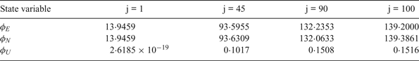
The misalignment angles ϕE and ϕN are totally observed through the whole process. In the first time segment, the observability degree of ϕU is less than 1, which is unobservable, and its degree of observability is very low; in the 100th time segment, the observability degree of ϕU improvement has been obviously improved, increasing from 2·6185 × 10−19 to 0·116. The results of observability degree analysis show that the erecting manoeuvre is conducive to enhancing the observability degree of some state variables, especially ϕU. The results of observability degree analysis show that the erecting manoeuvre is conducive to improving the system observability.
5. FINE ALIGNMENT EXPERIMENT
5.1. Experiment equipment and operation
To validate the proposed fine initial alignment method, three erecting experiments of a missile-borne INS were carried out. A high precision INS is developed with gyroscope drift and accelerometer bias which is better than 0·01°/h and 50 μ g, respectively (Li et al., Reference Li, Fang and Wu2014). The missile-borne INS is installed in a simulated missile with its Y-axis as the rotation axis of the erecting mechanism. When the launching vehicle arrived at the known launching location, it was stopped and attempted to be kept horizontal. The position vector of the rotating centre of the erecting mechanism O o in the navigation frame can be obtained through the GNSS receiver of the launching vehicle, which is  ${\bf P}_{o}^{n}=[\matrix{ L_{o} &\lambda_{o} &h_{o}}]^{T}=[\matrix{ 39{\cdot}797810^{\circ} &116{\cdot}410779^{\circ} &46{\cdot}426m}]^{T}$.
According to Equations (16) and (19), the lever arm vector is used to calculate the position and velocity measurements, and must be obtained before erecting alignment. The lever arm vector  ${\bf R}_{I}^{b}$ is measured by the laser total station instrument, and
  ${\bf R}_{I}^{b}=[\matrix{ 9{\cdot}161\,\hbox{m} &-0{\cdot}317\,\hbox{m} &0{\cdot}700\,\hbox{m}}]^{T}$. The lever arm is considered as a rigid lever arm and the length of the lever arm is unchanged during the whole experiment.
First, the initial attitude matrix of the missile-borne INS can be calculated by an analytical coarse alignment for ten seconds. Then, the fine alignment is performed during the erecting process. Using the erecting mechanism, the missile-borne INS is rotated 90° clockwise to the vertical state along the Y-axis within 100 s. The existing fine initial alignment method is performed on a stationary base after the missile-borne INS has been erected to the vertical state along the X-axis. The two alignment methods can be compared with each other. A set of optical measurement equipment including a laser tracker and a theodolite are used to measure the azimuth of the missile-borne INS in real time, and the result can be regarded as a reference for fine alignment.
5.2. Experiment results and analysis
The measurement equation of the proposed dynamic model is established through modelling and compensation of the lever arm effect. The position and velocity measurements are obtained in real time. According to Equations (18) and (20), measurements of the missile-borne INS can be calculated by three gyroscope outputs, the lever arm vector  ${\bf R}_{I}^{b}$ and the attitude matrix of INS
  $C_{b}^{n}$, which is independent of external equipment. The velocity and position measurements are given in Figures 3 and 4. The measurement equation of the existing method is available from the model of traditional self-alignment on a stationary base, and the measurements are constant.
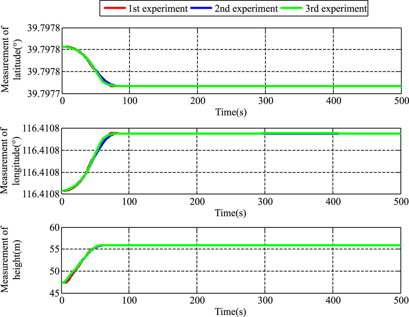
Figure 3. The measurement of position.

Figure 4. The measurement of velocity.
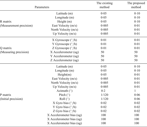
For the fine initial alignment, the Kalman filter parameters must be determined. According to the specifications of the missile-borne INS, the filter parameters can be obtained, as shown in Table 2.
Table 2. Parameters of Kalman filter used in the fine initial alignment.
Based on these filter parameters, three group fine initial alignment experiments have been carried out. Taking the azimuth measured by optical instruments as a reference, the azimuth errors obtained by the proposed method and the existing alignment method are given in Figure 5. Both alignment methods can obviously reduce the azimuth errors by a Kalman filter estimation to the requirement of precision which is δφ = 0·05°.

Figure 5. Azimuth errors operated by the proposed method and the existing method compared with the reference obtained by optical instruments.
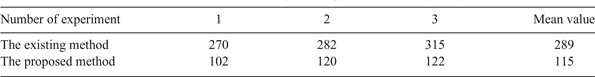
Compared with existing methods, the proposed method may not only share the erecting manoeuvre, but also improve the system observability. Therefore, the rapidity of the proposed alignment method is significantly better than the existing alignment method. Time consumption of the two fine initial alignment methods is given in Table 3. When the azimuth accuracy is better than 0·05°, time consumed by using the proposed alignment method is 115 s for three experiments, which is far less than 289 s consumed in the existing method. The experiment results prove that the proposed alignment method is faster and provides a valid solution.
Table 3. Times consumed by two alignment methods (unit: s).
6. CONCLUSIONS
In this paper, a fast fine initial self-alignment method of a missile INS is proposed, which is performed during the erecting process on a stationary base. The convected Euler angle error is modelled to optimise the erecting manoeuvre scheme which can prevent the large Euler angle error. Then, the fine alignment model is established to estimate and correct the initial misalignment. The observability degree was analysed by PWCS theory and SVD theory, which indicates the improvement of system observability. The proposed method may not only share the erecting manoeuvre, but also improves the system observability so that the alignment time can be reduced. The fine initial alignment experiments show that the rapidity of the proposed alignment method is significantly better than the existing alignment method, and proves the validity of the proposed method. It can contribute to the fast fine initial alignment of a missile-borne INS.
ACKNOWLEDGMENTS
The work described in the current paper was supported by National Natural Science Foundation of China under Grant 61571030, Grant 61722103 and Grant 61421063; in part by The National High Technology Research and Development Program of China (863 program) under Grant 2015AA124001 and Grant 2015AA124002; in part by Basic Scientific Research under Grant YWF-17-BJ-Y-71. The authors would like to thank all members of Science and Technology on Inertial Laboratory, Fundamental Science on Novel Inertial instrument and Navigation System Technology Laboratory for their useful comments regarding this work.


