


1. INTRODUCTION
The geolocation of moving platforms, that is, the accurate determination of their position coordinates at any time in some well-defined coordinate system, is an important aspect of most survey systems, where positional registration of collected data can vary in required accuracy from metres to millimetres. For example, the reliable detection of Unexploded Ordnance (UXO) and their discrimination from non-hazardous ferromagnetic objects depends not only on the sensor technology, but also on the precise geolocation data that are needed to invert the detection signals (Lee, Reference Lee2009). Positions at the precision levels of 1 cm to 10 cm and with high temporal resolution are necessary to map and characterize (discriminate) candidate UXO (Simms and Carin, Reference Simms and Carin2004; Bell, Reference Bell2005).
Where available, the Global Positioning System (GPS) or other similar Global Navigation Satellite System (GNSS) is the primary geolocation system for most survey platforms. It is aided by local systems in areas where satellite signal reception is obstructed or degraded. Typical aiding systems include local ranging (e.g. laser, radar, and acoustic systems) or completely autonomous sensors, such as Inertial Measurement Units (IMUs). In the case of UXO detection systems, navigation systems such as Real-Time Kinematic (RTK) GPS are unable to satisfy the strict position accuracy requirement in various challenging environments where signals from GPS are frequently blocked. Therefore, the primary geolocation system can be integrated with a three-dimensional IMU for potential improvement, but also to increase the temporal resolution of the geolocation capability. In this paper, we analyze the combination of a geodetic GPS receiver and two tactical-grade IMUs (Honeywell HG1700 and HG1900) that were deployed on each of two Naval Research Laboratory (NRL) UXO detection platforms: a vehicle-towed trailer and a cart-based system.
With two IMUs we have two solutions of the same vehicle trajectory, where each is combined with GPS using a filter. We test both the Extended Kalman Filter (EKF) and the Unscented Kalman Filter (UKF). In addition, the Wave Correlation Filter (WCF) is applied external to these filters because ideally the two inertial navigation solutions should be perfectly correlated, and differences would be caused only by errors. The WCF removes non-correlated spectral components using a pre-defined threshold. The two filtered solutions are averaged to give improved position estimates. Since both solutions are strongly affected by sensor biases that are not removed by the WCF, remaining error biases and trends of the estimated position are removed finally using an end-matching algorithm with respect to GPS updates points. Results of these methods applied to our field data are compared and analyzed.
2. METHODOLOGY
2.1. IMU Data Preprocessing
The performance of IMUs can be improved when the white noise of the sensors is removed in a pre-processing step. The medium-frequency band of the IMU data provides a good approximation of the navigation signal, while the high frequency part has few details of the signal and constitutes primarily noise. The separation of signal from noise is achieved by a wavelet de-noising technique that decomposes the IMU output into approximation (signal) and detail (noise) using a pre-defined wavelet transform (Nassar, Reference Nassar2003). The raw IMU data from HG1700 and HG1900 were de-noised using the Wavelet Multi Resolution Analysis (WMRA) method with the symlet ‘sym12’ wavelet (Daubechies, Reference Daubechies1992) up to level 4. Subsequently, this approximation of the IMU signal was employed in the Kalman filtering process.
2.2. Extended Kalman Filter (EKF)
The Kalman Filter (or EKF for nonlinear systems) is widely used to estimate positions of integrated IMU/GPS systems (Rogers, Reference Rogers2000; Jekeli, Reference Jekeli2000; Titterton, Reference Titterton and Weston2004). The Kalman Filter is an optimal, sequential, linear, least-squares estimation algorithm based on a priori statistics of the system states, that include, in the first place, the nine navigation states (three position errors (δxT), three velocity errors (δvT), and three orientation errors (δψT)). Since IMU errors include temporally correlated components, these states are typically augmented by states associated with biases and scale factor errors of gyroscopes (b gSg) and accelerometers (b aSa), among others. For the EKF all error states must be modeled appropriately using linear dynamics models. Collecting the states in the vector, εT=(δxT δvT δψT b gSg ba Sa), we write the linear error dynamics model as
where F is the dynamics matrix characterizing the time propagation of errors and u is a vector of normally distributed random variables, uncorrelated in time, scaled by the matrix G, and driving the dynamics of the error states (see the detailed F and G in Jekeli, Reference Jekeli2000).
The errors can be estimated by observations, y, that are linearly (or through linearization) related to them:
where H is the sensitivity matrix and v is the (white) noise in the observations.
The state estimation is optimal in the sense of least squares (Schaffrin, Reference Schaffrin and Sans`o1995; Jekeli, Reference Jekeli2000) and obtained recursively at discrete times, t k, according to
where Φk,k−1 is the state transition matrix from time t k−1 to t k. The innovation (actual minus predicted observations) in parentheses is scaled by the Kalman gain matrix, K k, which can be thought of as the ratio between the error covariance matrix of the estimates, P k, and the error covariance matrix of the observations, R: K k=P kHkTR −1.
2.3. Unscented Kalman Filter (UKF)
The UKF is a recursive application of the Unscented Transformation (UT) of state variables through the nonlinear state dynamics model (Julier and Uhlmann, Reference Julier and Uhlmann1996). The UKF differs from the EKF in that it propagates various deterministic sample states – not just the ‘predicted state’ as in Equation (4) – directly through the nonlinear system models in order to estimate the states and their covariance without requiring the linearization (Julier et al., Reference Julier, Uhlmann and Durrant-Whyte1995). Thus, it avoids the formulation and computation of derivatives of the system model. Because the EKF only uses the first-order terms of the Taylor series expansion of the nonlinear functions, it often introduces large errors in the estimated statistics of the posterior distributions of the states. This is especially important when the models are highly dynamic and the local linearity assumption breaks down (i.e. the effects of the higher-order terms of the Taylor series expansion of the system model become significant).
The UT propagates a suitably chosen set of sample points (sigma points) in the state space through the (nonlinear) system dynamics such that they accurately capture the transformed mean and covariance matrix of the state vector (Julier et al., Reference Julier, Uhlmann and Durrant-Whyte2000; Wan and van der Merwe, Reference Wan and van Der Merwe2001).
For an n-dimensional random variable x with mean, ![]() , and covariance, P, 2n+1 sigma points, χ i, of the UT are generated as follows
, and covariance, P, 2n+1 sigma points, χ i, of the UT are generated as follows

where α and κ are scaling parameters and ![]() is the i th row or column of the matrix square root of
is the i th row or column of the matrix square root of ![]() .
.
Given a nonlinear function, f(x), it can be shown that the following weighted combinations of z i=f(χ i), i=0 ,…, 2n, estimate the first two statistical moments (mean, ![]() , and covariance, P z) of f(x) very well, at least up to second order in the non-linearities:
, and covariance, P z) of f(x) very well, at least up to second order in the non-linearities:


with weights given by

The weights for the mean sum to unity, while for the covariance they sum to (1−α 2+β). The scaling parameter, α (10−4⩽α⩽1), controls the spread of the sigma points around ![]() and serves to maintain the positive semi-definiteness of the covariance (van der Merwe et al, Reference Van der Merwe, Doucet, de Freitas and Wan2000). For a Gaussian state vector, x, the estimation of the mean and covariance of f(x) is accurate up to third order. The parameter, β, is used to increase the accuracy of the higher-order moments.
and serves to maintain the positive semi-definiteness of the covariance (van der Merwe et al, Reference Van der Merwe, Doucet, de Freitas and Wan2000). For a Gaussian state vector, x, the estimation of the mean and covariance of f(x) is accurate up to third order. The parameter, β, is used to increase the accuracy of the higher-order moments.
2.4. Wave Correlation Filter (WCF)
The WCF ideally extracts common spectral components from two signals, while rejecting disparate ones, thus removing errors if the two signals are supposed to refer to the same source. Of course, common errors are not removed. With this filter we anticipate obtaining a more accurate positioning solution from the dual IMU measurements, where random errors left in the two final solutions should be uncorrelated and amenable to elimination or reduction by the WCF (a similar approach was used by Serpas, Reference Serpas2003 and by Li, Reference Lee2009 to improve solutions derived from independent data sets). Let the two EKF solutions along the trajectory be denoted ![]() and
and ![]() , respectively. The corresponding Fourier transforms are G 1(l) and G 2(l), where l is the wave number. The correlation coefficient, r l, per wave number is obtained by
, respectively. The corresponding Fourier transforms are G 1(l) and G 2(l), where l is the wave number. The correlation coefficient, r l, per wave number is obtained by
Each solution is filtered according to a pre-defined threshold:
The final position estimates are obtained by transforming the average of the retained frequency components back into the time domain:
where is F the Fourier transform.
2.5. End-Matching
The remaining trend and bias errors of both the EKF and UKF solutions after WCF processing were corrected by the end-matching method with respect to the GPS positions. In terms of latitude, longitude and height coordinates, the end-matching algorithm is a simple linear fit to given data at the ends of a free-inertial trajectory:
![$$\underbrace {\left[ {\matrix{ {\tilde \phi _r} \cr {\tilde \lambda _r} \cr {\tilde h_r} \cr}} \right] - \left[ {\matrix{ {\hat \phi _w} \cr {\tilde \lambda _w} \cr {\hat h_w} \cr}} \right]}_Y = \underbrace {\left[ {\matrix{ 1 & {(t - t_0 )} \cr 1 & {(t - t_0 )} \cr 1 & {(t - t_0 )} \cr}} \right]}_A\underbrace {\left[ {\matrix{ {b_0} \cr m \cr}} \right]}_X$$](https://static.cambridge.org/binary/version/id/urn:cambridge.org:id:binary:20151022042206496-0160:S0373463311000567_eqn11.gif?pub-status=live)
where ![]() are GPS points,
are GPS points, ![]() are the position after applying the WCF, and b 0 is a bias and m is the trend.
are the position after applying the WCF, and b 0 is a bias and m is the trend.
The remaining bias and trend (vector X) error can be found by least-squares estimation
3. TEST AND ANALYSIS
The described methods were evaluated using IMU/GPS data from field tests conducted at NRL's UXO test site located at the Army Research Laboratory Blossom Point Facility in Maryland with the Multi-sensor Towed Array Detection System (MTADS), (Figure 1a) and a cart-based system (Figure 2). At the centre of MTADS we mounted OSU's dual-IMU/GPS system (Figure 1c): two tactical-grade IMUs (HG1700 and HG1900) in the IMU box (Figure 1b), one Topcon geodetic GPS receiver (GB-1000), and a laptop computer for data collection and communication with the sensors. The cart-based system has only OSU's IMU/GPS system and one large 12 V battery for power (Figure 2).

Figure 1. (a) The NRL Multi-sensor Towed Array Detection System (MTADS), (b) IMU box, (c) OSU's dual-IMU/GPS system.
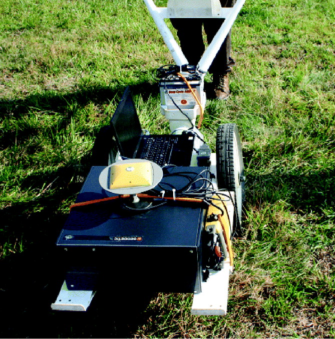
Figure 2. The NRL cart-based system with OSU's dual-IMU/GPS geolocation system.
Eight field tests were performed using the two platforms and various GPS satellite configurations. Among these tests, GPS malfunctioned for one complete test, and three tests were designed for deliberate GPS degradation (near a wooded area). Thus, we considered only the four Tests 2, 5, 6, and 7 in this analysis. They were divided into two test scenarios (Scenario 1: Tests 2 and 5, Scenario 2: Tests 6 and 7) according to the number of visible GPS satellites. The GPS Geometric Dilution of Precision (GDOP) for Scenario 1 was lower than that for Scenario 2.
The test range is roughly 84 m long by 24 m wide. The vehicle-towed trailer and cart-based system were moved along trajectories that are typical of a UXO survey. At the end of each trajectory segment there are large turns to align the platform to the next straight segment of the trajectory.
Figure 3 shows the GPS trajectories of the vehicle-towed trailer and the cart-based system for Scenario 1 (Test 2, MTADS; Test 5, Cart) and Scenario 2 (Test 6, Cart; Test 7, MTADS). The total distance of Test 2 (Test 5) is about 2,016 m (398 m) and the speed of the MTADS (Cart) is about 1·85 m/s (0·95 m/s). The total distance of Test 6 (Test 7) is about 352 m (514 m) and the speed of the Cart (MTDAS) is about 1·0 m/s (1·9 m/s).

Figure 3. The GPS trajectory of the vehicle-towed trailer and Cart-based system (Tests 2 and 5 are Scenario 1 and Tests 6 and 7 are Scenario 2).
The kinematic GPS analysis package ‘KinTOOLS’ was used to process 1 Hz GPS data collected by the Topcon GB-1000 receiver. The proximity to the base station (less than 1 km) allowed us to use a single-frequency L1 analysis. We also computed the L1-L2 combined frequency solution and we found the L1 solution to be sufficient and robust with less noise than the combined solution. Each trajectory using the individual inertial sensors was estimated by the EKF or the UKF and then the WCF was applied to the common solutions with the threshold value of 0·5 (Equation (10)). The remaining bias and trend errors are further removed by the end-matching method. Figure 4 illustrates the general IMU/GPS data processing and analysis procedure.

Figure 4. IMU/GPS Data Processing Flowchart.
3.1. Scenario 1
The filtered free-inertial (IMU-only) positions of the vehicle-towed trailer and cart-based system were computed along the straight sections within 2, 4, and 6 second intervals representing artificial periods of GPS unavailability. Figure 5 illustrates parts of the estimated positions from the trajectory of Test 2.

Figure 5. The estimated vehicle trajectory using GPS, the HG1700 w/ UKF the WCF, and end-matching, for different update rates.
As the interval between GPS updates increases from 2 to 6 seconds, the IMU-estimated position (HG1700) using the EKF with WCF and end-matching is demonstrably better than the position using just the EKF and the EKF with WCF. Similar improvement was obtained with the WCF applied to the UKF solutions.
Figure 6 shows the standard deviations of position errors of the three coordinates (based on all straight sections of the trajectory) of Tests 2 and 5 according to the UKF, the WCF estimates based on the UKF solutions, the estimates obtained by applying the UKF, the WCF, and end-matching, and the Unscented Kalman Smoother (UKS) (see Annex for detail derivation). We show only the UKF-only estimates for the HG1700 because it yields better position accuracy than the HG1900.
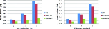
Figure 6. The standard deviation of position error in the straight section according to the UKF, the UKF with WCF, and the UKF with WCF and end-matching based on the UKF solutions (left: Test 2, right: Test 5).
Test 5 (Cart-based system) yielded overall better performances than Test 2 (vehicle-towed trailer) because the cart-based system experienced lower dynamics and slower speed than the vehicle-towed trailer. The WCF with end-matching improved the UKF solutions (control updates every two points) of Test 2 by about 46%, compared to an 11% decrease in the standard deviation of errors without the end-matching. Also, the WCF with end-matching improved the UKS solutions (control updates every two points) of Test 2 by about 5%.
In the 4 and 6 second GPS outage cases, the position errors (standard deviations) decreased 64% and 76% with respect to the UKF-only errors, 55% and 70% relative to the UKF with WCF, and 9% and 14% respect to the UKS. In Test 5, the position errors with the WCF and end-matching decreased about 52%∼69% with respect to the UKF-only solutions, 46%∼64% with respect to the UKF plus WCF solutions and 4%∼10% with respect to the UKS considering all 2, 4, and 6 second GPS outages.
3.1. Scenario 2
In Scenario 2 (Tests 6 and 7), the number of GPS satellite increased from 4∼5 to 7∼8, and the PDOP correspondingly decreased from 4·3 (Test 5) to 2·6 (Test 6). Similar to Scenario 1, the WCF and end-matching improved the performances of the UKF in all straight sections (Figure 7). In Test 6 (Test 7), the position errors with the WCF decreased about 52%∼69% (50%∼73%) with respect to the UKF-only solutions, 44%∼63% (43%∼67%) with respect to the UKF with WCF solutions, and 4%∼13% (4%∼12%) with respect to the UKS considering all GPS outages.

Figure 7. The standard deviation of position error in the straight section according to the UKF, the UKF with the WCF, and the UKF with the WCF and end-matching based on the UKF solutions (left: Test 6, right: Test 7).
4. CONCLUSION
The combination of two IMUs and a GPS receiver has been employed to address the precision geolocation needs for survey platforms, such as a UXO detection and discrimination system. Application of the WCF with end-matching to the two individual IMU solutions in field tests and, based on the UKF (UKS), demonstrated the ability to improve the position accuracy of the geolocation system. The standard deviations of the position errors of the UKF (UKS) were reduced from 52 (4)% to 75 (14)% for a vehicle-towed platform, and from 50 (4)% to 69 (13)% for a cart-based system, while GPS was unavailable for up to 6 seconds. The improved geolocation accuracy will enhance geophysical data inversion performance and will decrease substantial UXO remediation cost.
ANNEX
Unscented Kalman Smoother (UKS)
The Unscented Kalman Smoother (UKS) is based on the application of the Rauch-Tung-Striebel (RTS) smoothing algorithm to the UKF. A summary of the UKS starts with the propagation of the sigma points through the dynamic model (see Sarkka (Reference Sarkka2008) for more detailed derivations)
where ![]() denotes the sigma point i, which corresponds to x k.
denotes the sigma point i, which corresponds to x k.
For the next step, compute the predicted mean, the predicted covariance and the cross-covariance
where the definitions of the weights are the same as for Equation (7)
Finally, compute the smoother gain, the smoothed mean and the covariance
This is a recursive procedure. It can be used for calculating the smoothing distribution of step k from the smoothing distribution of time step k+1. The initial conditions for k=N are:
ACKNOWLEDGEMENTS
This study was supported by SERDP project MM-1565, contracts W912HQ-07-P-0013 and W912HQ-08-C-0044. We would like to thank Daniel A. Steinhurst and Glenn R. Harbaugh, both at the Naval Research Laboratory (NRL), for helping conduct our field tests at NRL's UXO test site.


