1. INTRODUCTION
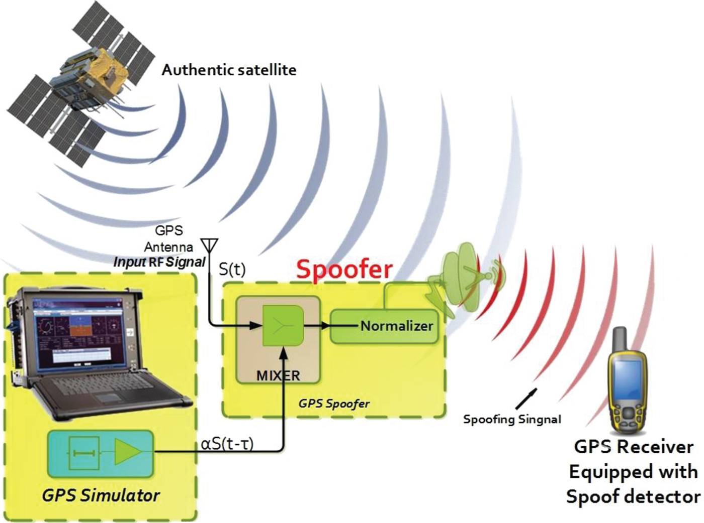
The importance of applying security to telecommunication and electronic systems has increased significantly, leading to various signal protection methods. Global Positioning System (GPS) signals should be protected against attacks and GPS spoofing attacks attempt to deceive a receiver by broadcasting counterfeit signals. The spoofing signals are usually slightly stronger than authentic signals. They may be generated by a delay and re-emission of an authentic reserved GPS signal (Baziar et al., Reference Baziar, Moazedi and Mosavi2015).
Figure 1 illustrates an in-process spoofing attack. A spoofer can produce incorrect navigation data for the GPS receiver by taking the receiver correlation peak (Jovanovic et al., Reference Jovanovic, Botteron and Farine2014). Figure 2 shows the tracking loop of the target receiver at four moments (T1-T4) during a spoofing process. As can be seen, the spoofer transmits a fake signal to the target receiver in either a synchronous (row A) or an asynchronous (row B) manner. Multipath (MP) exists in all parts of the figure. Five correlation taps are investigated (very Early (VE), Early (E), Prompt (P), Late (L) and very Late (VL)). In a locked condition, the “VE” tap equals to “VL” and the “E” tap equals the “L” tap. In a synchronised attack, the spoofer is aware of the phase centre of the receiver antenna. The forged signal remains hidden while the authentic signal is under control. At first, the amplitude of the spoofing signal (SPOOF) is smaller than the original Line-of- Sight (LOS) signal (T1). After a while, the correlation peak of SPOOF increases slowly (T2) and is finally adapted to the LOS peak (T3). After that, the SPOOF starts to control the tracking loop (T4).

Figure 1. GPS receiver's deviation from the original path.
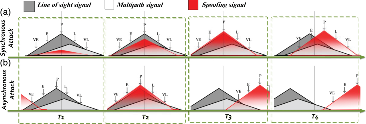
Figure 2. Two different spoofing scenarios with the correlation region types in tracking loop: (a) synchronous spoofing and (b) asynchronous spoofing.
On the other hand, in asynchronous attacks, SPOOF is not aligned with LOS. SPOOF power is originally higher than LOS (T1). The LOS peak approaches the SPOOF peak in steps (T2). After interaction of two peaks (T2) the target receiver ignores the LOS (T3) and SPOOF starts to direct the receiver (T4). It is worth noting that a synchronous attack is difficult to implement and an asynchronous attack is a more realistic scenario (Bonebrake and O'Neil, Reference Bonebrake and O'Neil2014; Humphreys et al., Reference Humphreys, Ledvina, Psiaki, O'Hanlon and Kintner2008).
A variety of solutions have recently been presented for detection and reduction of spoofing attacks. One of the methods in this field considers the receiver Carrier-to-Noise (C/No) ratio for identifying any spoofing by abnormal and sudden changes in the received signal (Jahromi et al., Reference Jahromi, Broumandan, Nielsen and Lachapelle2012a). Under standard weather conditions, only ionosphere changes and satellite movements may make gradual modifications in the received power (Jahromi et al., Reference Jahromi, Broumandan, Nielsen and Lachapelle2012b).
Presence or absence of a spoofing attack can also be detected by statistical hypothesis tests (Cavaleri et al., Reference Cavaleri, Motella, Pini and Fantino2010). For example, the Signal Quality Monitor (SQM) method can effectively detect abnormal sharp signal peaks and the overlapped peaks which approach the authentic signal. However, they are not applicable in cases where a spoofing attack does not affect the shape of the correlation peak. This situation happens when counterfeit and authentic signals are almost aligned (Pini et al., Reference Pini, Fantino, Cavaleri, Ugazio and Presti2001). To improve the performance of the SQM method, several approaches, such as Vestigial Signal Defence (VSD), Vector Based (VB), and a combined technique have been suggested.
VSD is a method based on the supervision of destruction of complex correlation. Performance of this method depends on the weakness of authentic GPS signals during a spoofing attack (Wesson et al., Reference Wesson, Shepard, Bhatti and Humphreys2011). In the VB method, the output including five correlator branches are exploited in a statistical hypothesis test to detect spoofing. If all the correlator branches are less than the threshold, the signal will be authentic. Although this method is efficient, it increases the complexity of hardware and processing. Two extra correlation taps in the tracking loop and a feature extraction segment are needed. Additionally, the use of the χ2-test and determining the threshold level have particular complexity (Lashley and Bevly, Reference Lashley and Bevly2009; Jahromi et al., Reference Jahromi, Lin, Broumandan, Nielsen and Lachapelle2012c).
Choosing the valid signal based on Signal to Noise Ratio (SNR) characteristics combined with a decision rule is used to counter a spoofing attack. These approaches are simple to implement, but not reliable. Some types of spoofing attack deceive a victim receiver into reporting a counterfeit position without significantly changing the SNR of the signal, such as attacks that distort the received correlation profile or change the pseudo-range of some satellites. Since generating these attacks are not difficult, achieving a secure GPS receiver based on only this approach is not possible (Nielsen et al., Reference Nielsen, Dehghanian and Lachapelle2012). Some methods constantly investigate compatibility of GPS signals by supplementary equipment including Inertial Measurement Units (IMUs) and the positioning information gathered from wireless local network stations or mobile networks for spoofing threat detection. In this way, auxiliary equipment positioning information can be used to separate the spoofing threat. If different methods result in incompatible positions, spoofing is probable. The main problem of this technique is the complexity of hardware and software of GPS receivers. It is obvious that extra equipment imposes more cost to the navigation process (Niedermeier et al., Reference Niedermeier, Beckmann and Eissfeller2012). IMU sensors need calibration before use (Petovello, Reference Petovello2003). Wireless positioning technology such as cellphone networks requires additional equipment. Besides, the mentioned technology does not offer a positioning solution with the same accuracy as a GPS signal.
Ochin et al. (Reference Ochin, Dobryakova and Lemieszewski2012) detected spoofing by recognising statistical incompatibility while analysing the specifications of satellite signals. The main problem with this technique is the availability of authentic signal information before starting an attack. In fact, after a spoofing attack, the specifications of the spoofing signal are placed in the allowed threshold level. Adaptation and estimation of the input signal is an approach that extracts the GPS signal characteristics. In this method, any unexpected or significant change represents an occurrence of a spoofing attack (Humphreys et al., Reference Humphreys, Psiaki, Kintner and Ledvina2006).
Simple and intermediate spoofers transmit multiple spoofing signals from one antenna, while the valid GPS signals from different satellites arrive from different directions (Nielsen et al., Reference Nielsen, Broumandan and Lachapelle2010). This can be used to estimate the effect of Three-Dimensional (3D) spatial processing of received signals based on the antenna array (Montgomery et al., Reference Montgomery, Humphreys and Ledvina2009a; Reference Montgomery, Humphreys and Ledvina2009b). This technique is reliable but takes more computation, time and results in hardware complexity. Moreover, this method increases the receiver dimensions, and may not be easy to implement in common civil receivers.
It is apparent that a more accessible low cost and reliable technique with higher accuracy is required. In recent years, artificial intelligence techniques have been used to control a broad range of systems (Mosavi and Shafiee, Reference Mosavi and Shafiee2016). This paper presents a new spoof recognition method implemented in a GPS Software Defined Receiver (SDR). The proposed algorithm utilises Neural Networks (NNs) to recognise abnormal distortions of correlation for spoofing detection. As will be shown later, by applying NN, the signal index moves beyond the allowed threshold level and spoofing is recognised when the attacker wants to occupy the receiver's correlation peak. The offered method needs no extra hardware and does not increase the receiver size or production cost. In our approach, there is no necessity for any authentic signal after training.
To better comprehend the proposed algorithm, initially it is required to explain collection of the utilised data set for feature extraction and classification. This will be explained in the next section. After that, GPS spoof signal pattern recognition and feature extraction are discussed in Section 3. The required features for classifier algorithms are provided in this step. Section 4 explains the proposed method. After a general description of the suggested algorithm, two conventional approaches are studied. Finally, the detailed description of our suggested technique is discussed. In Section 5 an evaluation with experimental results and comparison with other methods are reported. Finally, Section 6 concludes the work.
2. GPS SIGNAL DATA COLLECTION
To test the proposed approach, delay spoofing is generated. The original data collection process records authentic signals from GPS satellites. These signals are reinforced and sampled in the 5·7 MHz rating at the front-end. After down-conversion to an Intermediate Frequency (IF), filtering and Analogue-to-Digital Conversion (ADC), the sampled time-discrete signal is fed into a SDR (Baziar et al., Reference Baziar, Moazedi and Mosavi2015).
Figure 3 shows the hardware equipment used for data collection. As can be seen, signals received from the GPS antenna are combined with signals generated by a GPS simulator after an appropriate delay. The resulting signal is applied to a front-end which prepares the proper two-bit digital signal for the SDR. Then, the sampled spoofing signal enters the acquisition and tracking sections of the SDR equipped with the proposed anti-spoofing algorithm. The following formula is the model of the GPS spoofing signal (Baziar et al., Reference Baziar, Moazedi and Mosavi2015):
 $$R_{C/A} (t) = A_{C}^{A} (t) C_{i}^{A} (t) D_{i}^{A} (t) \sin (w_{L1} t + \varphi_{L1}^{A}) + A_{C}^{D} (t) C_{i}^{D} (t) D_{i}^{D} (t)\sin (w_{L1} (t - \Delta t_{D}) + \varphi_{L1}^{D})$$
where A C , C i , and D i represent amplitude, Coarse/Acquisition (C/A) code and navigation data, respectively. Also, indexes A, D, L1, and i denote the authentic signal, delayed signal, L1 channel carrier and number of GPS satellites, respectively. w L1 is the angular frequency of the L1 signal, φ L1 is L1 signal phase and Δ t D is the delay of the counterfeit signal. To hide a valid GPS signal at the receiver, the power of the spoofing signal must be increased. The deception process generates a delayed signal as shown in Figure 4 (Lo and Enge, Reference Lo and Enge2010). The yellow boxes show a schematic of the hardware in Figure 3.
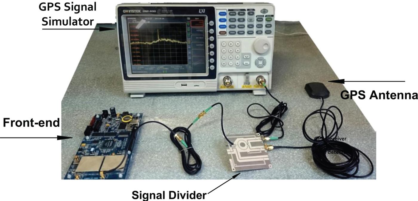
Figure 3. GPS hardware used for data collection.

Figure 4. Scheme of delayed spoofing GPS.
3. SPOOF SIGNAL PATTERN RECOGNITION AND FEATURE EXTRACTION
Spoof signal pattern recognition is a methodology which exploits various categories of features. When the spoof signal correlation peaks are close to the original signal correlation peak, the extracted features of the spoof pattern are used to detect the signal type. As can be seen in Figure 5, phase and amplitude matching does not occur in spoof and authentic signals. Multipath signals are delayed with attenuated amplitude. M 1 and M 2 are the first and second multipath components, respectively. Other components such as ionospheric disturbances are not considered since their attenuation is high.
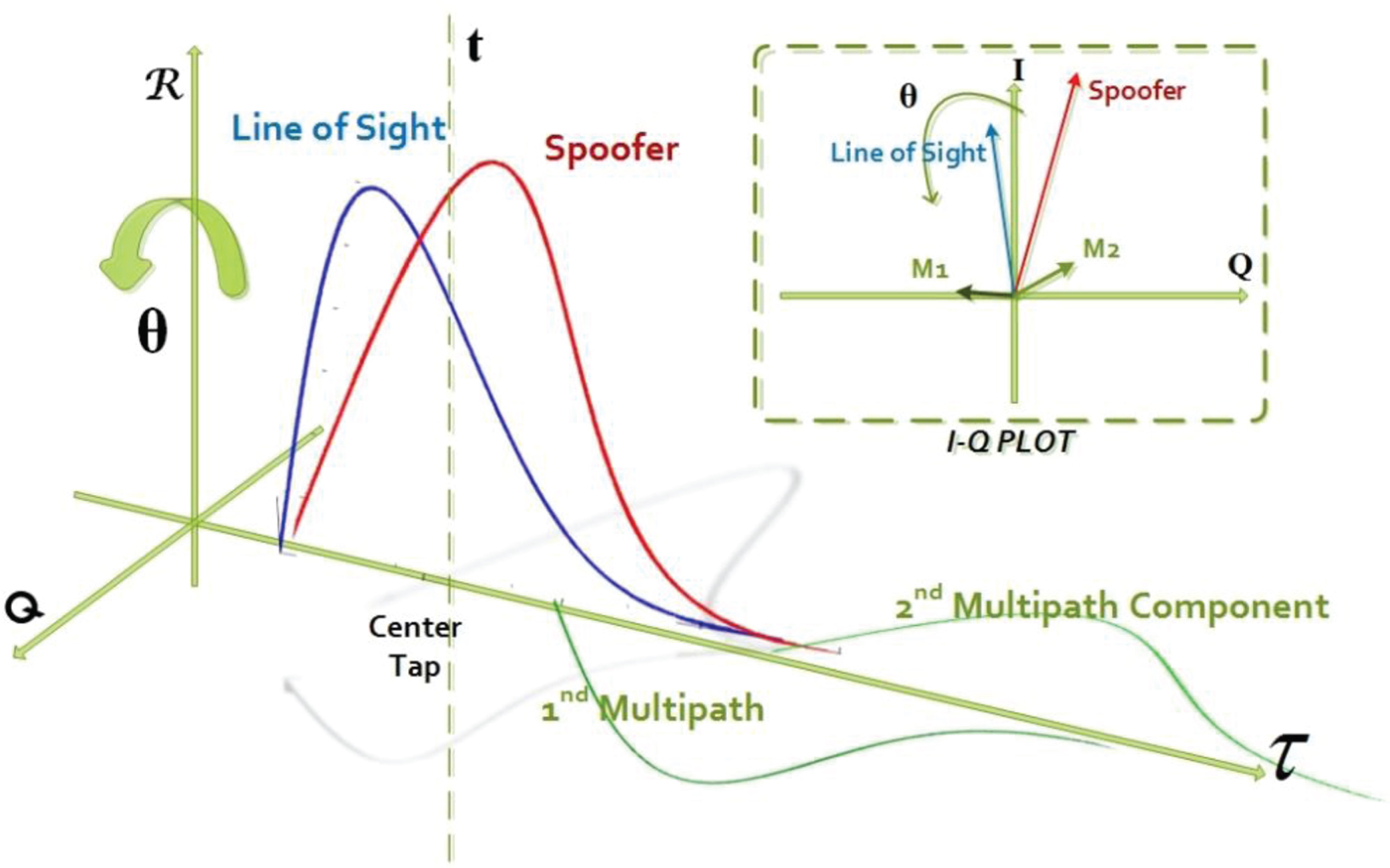
Figure 5. GPS signal with spoofing and multipath signals (the spoofing attack complex correlation scope, In-phase and Quadrature plots).
Equations (2) and (3) represent the signals shown in Figure 5. It is difficult for a spoof attacker to adapt the spoofing signal carrier phase with an authentic signal. If the correlation of the produced C/A signal is obtained by total input signal, a complex correlation function x in time t and offset delay τ can be calculated (Wesson et al., Reference Wesson, Shepard, Bhatti and Humphreys2011).
 $$\eqalign{ x(t, \tau) &= x_{d} (t, \tau) + x_{m} (t, \tau) + x_{S} (t, \tau) + \eta (t, \tau) }$$
 $$\eqalign{ x(t, \tau) &= \alpha_{d} (t) R (\tau - \tau_{d} (t)) e^{\,j\theta_{d} (t)} + \sum\limits_{k=1}^2 {\alpha_{m,k} (t)R(\tau -\tau_{m,k} (t))} e^{\,j\theta_{m,k} (t)} \cr &\quad + (\alpha_{\rm S} (t) R(\tau - \tau_{d} (t))e^{\,j\theta_{s} (t)}) n_{spoofing} + \eta (t, \tau) }$$
In Equation (2), x
d
indicates the LOS signal correlation function (original authentic GPS signal). x
m
indicates multipath elements (M1 and M2 in Figure 5), x
s
is a spoofing signal and η is additive white Gaussian noise. In Equation (3), R(τ) shows complex correlation and
 $0 \le \alpha \lpar t\rpar \le l$
is an amplitude factor. τ
d
(t) is the time delay in seconds. Phase θ (t) is expressed in radians, which vary with time and n
spoofing
shows the number of the spoofer.
$0 \le \alpha \lpar t\rpar \le l$
is an amplitude factor. τ
d
(t) is the time delay in seconds. Phase θ (t) is expressed in radians, which vary with time and n
spoofing
shows the number of the spoofer.
Ignoring
 $\eta \lpar t\comma \; \tau\rpar $
and x
m
(t), the discussion that follows in the rest of this section aims at exploring a way to recognise that the received signal only includes x
d
(t) or is a collection of x
d
(t) and x
s
(t). In other words, it is assumed that for any input signal there are two classes: spoofing
$\eta \lpar t\comma \; \tau\rpar $
and x
m
(t), the discussion that follows in the rest of this section aims at exploring a way to recognise that the received signal only includes x
d
(t) or is a collection of x
d
(t) and x
s
(t). In other words, it is assumed that for any input signal there are two classes: spoofing
 $\lpar x_{d} \lpar t\comma \; \tau\rpar + x_{S} \lpar t\comma \; \tau\rpar \rpar $
and authentic x
d
(t, τ).
$\lpar x_{d} \lpar t\comma \; \tau\rpar + x_{S} \lpar t\comma \; \tau\rpar \rpar $
and authentic x
d
(t, τ).
The basis of classification in this study is the features of signal vectors. These features are the phase, energy and correlation distribution function extracted from the output of the correlator branch. The first step is to obtain a complex correlation function (I-Q vectors) by data extraction from the output including three correlators. The selected features compose classes with low correlation and high variance The delta criterion, the coefficient of early and late phase criterion and the total levels of signal are considered as the features. The first feature is the delta criterion (X1) calculated as (Wesson et al., Reference Wesson, Shepard, Bhatti and Humphreys2011):
 $$x_{1} = \Delta_{\tau} (t) = \displaystyle{{I_{E,\tau} (t)-I_{L,\tau}(t)}\over{2I_{p} (t)}}$$
where I E, τ (t) and I L, τ (t) are the real part of the former and latter correlation indices, respectively which are above and below the main branch I p (t) in the phase element by τ seconds. The second input is early and the late phase criterion and is calculated by (Wesson et al., Reference Wesson, Shepard, Bhatti and Humphreys2011):
 $$x_{2} = ELP_{\tau} (t) = \tan^{-1} \left(\displaystyle{{Q_{L, \tau} (t)}\over{I_{L, \tau} (t)}} - \displaystyle{{Q_{E, \tau} (t)}\over{I_{E, \tau} (t)}} \right)$$
where Q E, τ(t) and Q L, τ(t) are early and late branches which are earlier and later than I p (t) in the square of the element in time t by τ seconds. Finally, the third input is the signal level:
 $$x_{3} = SL = \displaystyle{{1}\over{T}} \int_T {\vert x(t, \tau) \vert^{2} d \tau}$$
This equation calculates the normalised value of correlation function integration, which is the normalised energy of the process. After determining the input indices, the data features are normalised in equations between −1 and 1.
 $$x_{scale} = x_{input} \cdot S + O$$
 $$S = \displaystyle{{x_{hi} - x_{low}}\over{x_{max } - x_{min}}},\quad O = \displaystyle{{x_{max} \cdot x_{low} -x_{min} \cdot x_{hi}}\over{x_{max} - x_{min}}}$$
where S and O are scale and deviation coefficients, respectively. Parameters of x min and x max determine the minimum and maximum of the input data, and x hi and x low are the range of scale.
Figures 6 to 8 show the three inputs described above. It is obvious that a spoofing signal has a different behaviour in comparison with an authentic signal in the early-late phase since the spoofing signal has failed to keep the phase adaptation with the authentic signal that requires a spoofer to be close enough to the receiver antenna phase centre. A spoofer needs a signal level higher than an authentic signal to keep the GPS receiver correlation peak as shown in Figure 5.
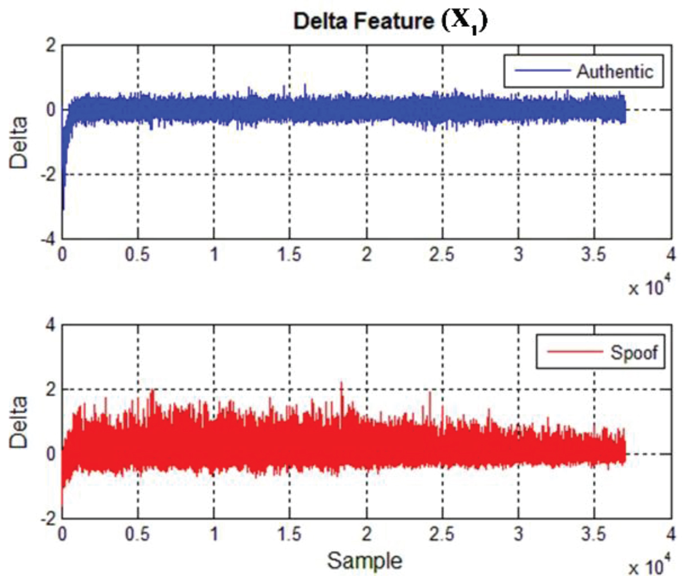
Figure 6. Delta feature (X 1) (the difference between early and late phase to In-phase ratio).
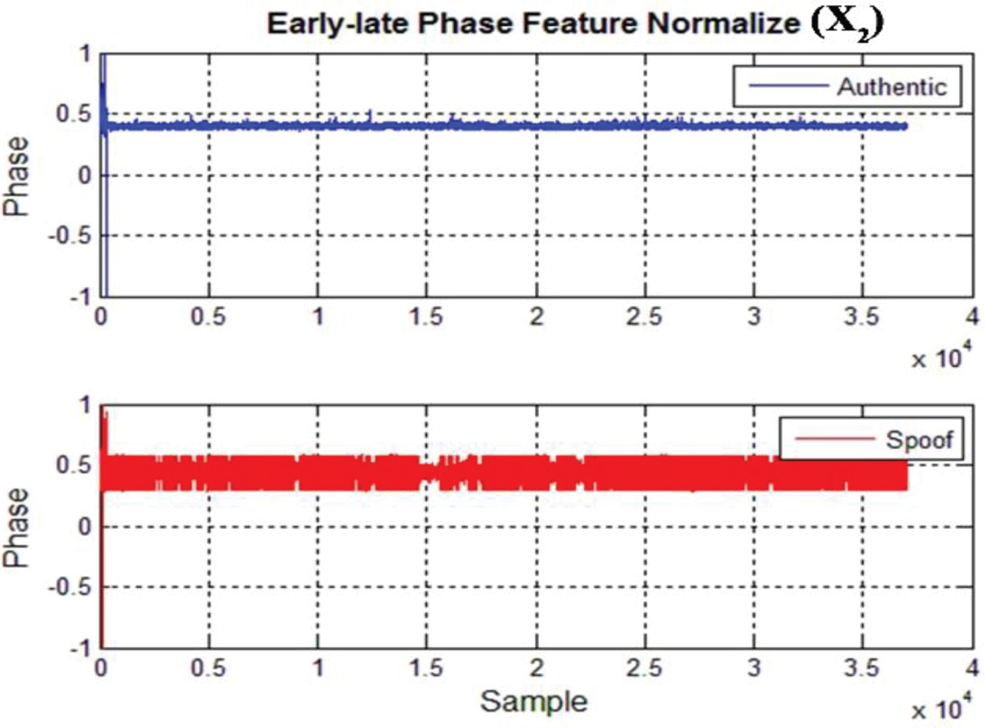
Figure 7. Early-late phase feature (X 2) (normalised phase in radians).
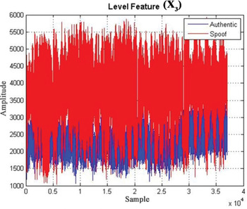
Figure 8. Signal level feature (X 3).
4. GPS SPOOFING DETECTION METHODS
The classifiers to be explained here are the K-Nearest Neighbourhood (KNN) classifier, the naive Bayesian classifier, and the proposed recognition method based on NN.
4.1. K-Nearest Neighbourhood Classifier
KNN is a simple algorithm that stores all available samples and classifies a new sample based on a similarity measure with a spoof signal in the delta, early-late and signal level features. By measuring the distance between the new sample and samples in memory, its class can be estimated (Kantardzic, Reference Kantardzic2003). A case is classified by a majority vote of its neighbours, with the case being assigned to the class most commonly among its K-nearest neighbours measured by a distance function (Han et al., Reference Han, Pei and Kamber2011).
Here, the samples are signal features and two classes exist; spoofing and authentic. The first issue is introducing proper criteria to recognise the distance of signals. In this case, a feature vector and Euclidean distance can be used. Each feature determines a dimension and the sample vector of the signal is the value of each feature in every dimension. The problem of this method is a slow training process. If this step is implemented without evolutionary or mathematical algorithms (Hassanat et al., Reference Hassanat, Abbadi, Altarawneh and Alhasanat2014), the complexity will be n 2 where n is the number of samples.
The feature space, training data and K value can influence classification accuracy. K is constant and should be previously determined. A small K increases noise sensitivity and with a large K, a neighbour may be included in more than one class (Bhatia and Vandana, Reference Bhatia and Vandana2010). Therefore, after deciding different values for K, we use the validation process.
One method employed in prediction applications is cross-validation which divides the data into two groups, training and test data. The analysis is implemented on training data, while validation is implemented on test data. To decrease discrepancies, validation is usually repeated and the results are averaged.
K-fold is an efficient method for cross-validation (Ma et al., Reference Ma, Yang and Cheng2014). The KNN algorithm can be implemented as:
-
1 The best positive integer K is specified along with a new sample (see Figure 9).
-
2 Select K entries in our database which are closest to the new sample (see Figure 10).
-
3 Find the most common classification of these entries.
-
4 This is the classification given to the new sample.

Figure 9. Error value by increasing the number of neighbourhoods.
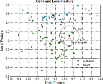
Figure 10. Prediction of new sample class based on delta and level features.
K-fold cross-validation is one way to achieve a better result than the “leave one out” method. The data set is divided into K subsets, and the leave one out method is repeated K times (Arlot and Celisse, Reference Arlot and Celisse2010). Each time, one of the K subsets is used as the test set and the other K-1 subsets form a training set. The loss value for two methods of K-fold and re-substitution (resub) is shown in Figure 9 for different numbers of K. K-fold loss is the error of K-fold cross-validation and resub-loss returns the classification loss by resubstituting. As can be seen in Figure 9, the minimum loss obtained with K-fold is K = 15, but for this K the resub-loss is high. Therefore, K = 13 is selected as a number for which both methods have a low loss equal to 0·02. Because we test the algorithm with replaced data, the resub-loss method is not as good as K-fold. After repeating the simulation several times, 0·0467 is selected as the worst achieved loss. 0·0467 is considered to be a high error value. Moreover, the main problem of the K-fold algorithm is high dependence on the training data and the value of K. Unpredictable conditions are created for new features, decreasing the robustness of the KNN algorithm.
4.2. Naive Bayesian Classifier
This classifier is based on Bayes' theorem with independent assumptions between the predictors. A naive Bayesian model is easy to build, with no complicated iterative parameter estimation which makes it particularly useful for very large data sets.
Bayesian-based methods are good for recognising the nature of a signal but are sensitive to the initial parameters. Moreover, they need adequate training based on initial knowledge about probability values. In the next stages, acquired data is utilised and signal properties are categorised based on their probability of occurrence. This information should be approximated if it is not available. For this purpose, prior knowledge from collected data helps in considering assumptions about probability distribution.
From a mathematical view, this method has a little risk. Bayes' theorem provides a way of calculating the posterior probability P(c | x) from P(c), P(x), and P(x | c). The naive Bayes classifier assumes that the effect of the value of a predictor (x) on a given class (c) is independent of the other predictor values. This assumption is called class conditional independence (Burmana, Reference Burmana1989):
 $$P(c\vert x) = \displaystyle{{P(x\vert c)P(c)}\over{P(x)}}$$
where P(c) is the prior probability of class, P(x) is the prior probability of the predictor, P(c | x) is the posterior probability of the predictor (class c) given attribute (x) and P(x | c) is the likelihood and the probability of the predictor given class.
Signal features are important for this classifier. The basis of its operation is that the probability of some features in a specific signal is higher. This method introduces an example dataset which acts as a high probability spoofing signal. Three calculated features from the previous section can be seen in Figure 11. These features are used in the Bayesian classifier algorithm. x(x
1, x
2, x
3) is a new sample vector feature of the GPS signal whose components are classification features. New observation x belongs to class Cj if its probability of belonging (posterior probability,
 $P\lpar Cj\vert x\rpar \rpar $
is greater than the probability of belonging to other classes. This can be expressed as:
$P\lpar Cj\vert x\rpar \rpar $
is greater than the probability of belonging to other classes. This can be expressed as:
 $$j = \mathop{arg \ max}\limits_{x_k} \prod\limits_{k=1}^3 P\lpar x_{k} \vert C_{j} \rpar \cdot P\lpar C_{j} \rpar \Rightarrow x_{k} \in C_{j}$$
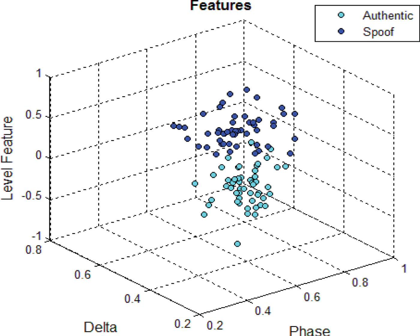
Figure 11. 3D plot of features (x 1, x 2, x 3).
To obtain positioning parameters, 37,000 samples with a 5·7 MHz sampling rate are required. Classification performance can be analysed in a 2 × 2 confusion matrix including True Positives (TP), False Positives (FP), False Negatives (FN) and True Negatives (TN). In our problem, positive means authentic signals and negative means spoofed signals. In this way, the (1,1) element, TP, is the number of correctly detected authentic samples and the (2,2) element, TN, is the number of correctly detected spoofing samples. The (1,2), FP, reports the number of falsely detected authentic signals Finally, the (2,1) element, FN, reports falsely detected spoofing samples. It can be concluded that the first and second rows are respectively related to authentic and spoofed signals and off-diagonal elements indicate the classification error. Therefore, as this matrix changes into a diagonal matrix, better results are achieved in classification (Kantardzic, Reference Kantardzic2003). The training and test confusion matrix can be expressed as Equations (11) and (12), respectively. As expected, classification error in the training set is nearly zero.
 $$CM_{Train} = \left( {\matrix{ {36999} & 1 \cr 4 & {36996} \cr } } \right)$$
 $$CM_{Test} = \left( {\matrix{ {28860} & {8140} \cr {925} & {36075} \cr } } \right)$$
Here, two sets of the 37,000 samples with known class were used. As can be seen, the number of errors in the test phase is more than the number of errors in the training phase.
4.3. Design, Training and Validation of NN for Spoof Detection
Figure 12 shows the tracking loop of the SDR where the proposed detection algorithm based on Multi-Layer-Perceptron (MLP) NNs is implemented. The features are extracted from correlation outputs after the tracking loop locks. The NN is trained off-line and then tested and ready to use in the proposed algorithm. The investigation of the extracted features is done continuously. Detection of a spoofing signal generates an alarm for the user. While the spoofing exists, the process is repeated.

Figure 12. Proposed spoofing detection algorithm based on NN.
To utilise MLP NN, selection of the proper architecture and training algorithm is of great importance (Visa et al., Reference Visa, Ramsay, Ralescu and Knaap2011). Suitable architecture means selecting the optimal number of layers, the number of neurons in each layer and the proper activation function for each neuron (Azami et al., Reference Azami, Mosavi and Sanei2013). Here, the optimal structure is selected through a trial-and-error design process. Before applying NN for signal classification, the network should be trained. The designed NN system for spoofing detection has three criteria as its input space. It is trained with back propagation, Quasi-Newton, gradient descent and Levenberg Marqurardt (LM).
The results showed that LM has the best response in this application and is thus selected as the learning algorithm. The input layer is mapped onto the space of the signal classes or the output layer (Mosavi et al., Reference Mosavi, Mohammadi, M. Refan and Farrokhi2003). Hidden layers process the received information from the input layer and deliver it to the output layer. Each network is trained by receiving authentic and spoofing data. Several conditions are considered to stop the learning process. Time of learning or number of epochs pass a predetermined limit; gradient of error variations approaches to zero; error increases for several epochs. In this experience, network learning is being performed and the weighting coefficients between the layers are modified so that the difference between the predicted and measured values is acceptable. In this way, the learning process is completed by achieving this condition. The trained NN may be exploited for spoofing detection by a new collection of genuine GPS data. The LM training algorithm is a standard method for non-linear least squares problems with a rapid convergence. The LM algorithm is a combination of Newton-Gauss and maximum gradient descent and has the benefits of both mentioned algorithms. Therefore, the LM algorithm is used in this paper. In comparison with other algorithms, it has increased convergence speed, and lower computation and memory requirements (Mosavi, Reference Mosavi2007). Figure 13 shows a GPS receiver equipped with the anti-spoofing method. As can be seen, there is no change in receiver structure.
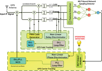
Figure 13. Vector-based GPS receiver structure with NN method.
The NN preparation procedure for spoofing detection unfolds as follows:
• First step
Compute complex correlation function of input signal in tracking loop (see Section 2).
• Second step
Three outputs of correlator branches are used by the feature extraction process. The features, delta criterion, early-late phase criterion coefficient and total level of normalised signal are extracted and used as the inputs of the MPL NN (see Section 3).
• Third step
The training algorithm is applied for classification according to the statistical properties of classes. Interpretation of classes is to be performed in this step. Finally, the MLP NN output analyser ascertains whether a spoofing attack is present or not.
5. ANALYSIS AND COMPARISION
To evaluate the designed NN algorithm, training and test data are sampled from two collections of spoofed and original data. The original data is authentic and collected in urban areas, while spoofing data is generated in the GPS laboratory of Iran University of Science and Technology as explained in Section 2.
After the NN is trained, GPS signals are tested to evaluate the classification method. The performance of the implemented NN is described by a confusion matrix. As described in Section 4.2, the classification is more effective if TP and TN elements are large. The Confusion Matrix (CM) for train and test data is observed as Equations (13) and (14), respectively.
 $$CM_{Train} = \left( {\matrix{ {29517} & {83} \cr {266} & {29344} \cr } } \right)$$
 $$CM_{Test} = \left( {\matrix{ {7362} & {38} \cr {78} & {7322} \cr } } \right)$$
From 37,000 samples, 80% are randomly selected for training and 20% for testing. It is worth noting that usually in algorithms which need to be trained, 70% of data is separated for training and 30% for testing (Mosavi, Reference Mosavi2007). As can be seen, 38 samples of spoofed signals are falsely selected as authentic signals and 78 authentic samples are falsely selected as spoofed data.
To evaluate accuracy, a series of indices are used for showing classification results, containing overall accuracy, Kappa coefficient, product accuracy, user precision, omission, and commission error. The dependency matrix information is summarised in the Kappa correlation coefficient. Overall accuracy is calculated by division of total signals which are classified correctly (TP) into the number of total signals. If the samples that are the true members of a category (TN and TP), are placed in other categories (FP and FN) while classifying the data, an omission error will happen. This error occurs when the vectors which are indeed the members of other classes are selected as members of the related class. This shows the process of changes of training parameters during training.
Figure 14 shows the variation of training error in each epoch. Until the eleventh epoch, the Mean Square Error (MSE) error of the NN significantly decreases. Training steps continue until the MSE error reaches five periods. This is the algorithm stopping condition selected by the trial-and-error process. Finally, if the slope is zero, the training can be stopped. As can be seen, the error remains 1·1262 × 10−5 for several epochs. More training data and epochs can increase the accuracy of classification, but the training time and over-fitting will probably be increased. After training (with correlation coefficient R value equal to 0·994), the classification error is extracted and shown in Figure 15 for the test data. Each circle represents a single sample. If the circles are on the line, the classification is done well. Circular deviation of the line indicates an error in the classification of the sample. Concentration of circles on 1 and 0 at the fit line demonstrates correct classification of the authentic and spoof groups. Similar to the confusion matrix in condition of false classification, the related circle inclines to other groups out of the fit line.
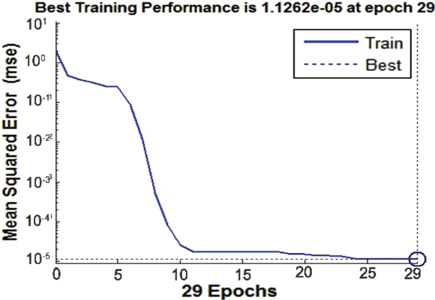
Figure 14. NN performance during training.
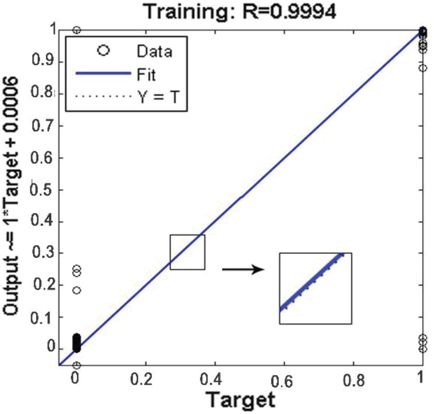
Figure 15. Classification error.
The SDR simulation was performed using MATLAB software in a computer with a dual-core 2·8 GHz CPU and 4 GB RAM. As can be seen in Table 1, the MLP NN was simulated by different architectures and eventually, an optimised structure (3-2-1) was chosen by a trial-and-error process. In this network, detection time is shorter with approximately equal error. The number of neurons in the first layer is equal to the number of three input indices. The number of neurons in the hidden layer and output layer is two and one, respectively. Thus, the network complexity is calculated using the following equation:
 $$Order = i \cdot j + j \cdot r + j + r = 11$$
where i, j, and r are the number of neurons in the input, hidden, and output layers, respectively. MSE in this table refers to the average of recognition mistakes by trained NN output. Low MSE indicates that the MLP NN usually selects the correct class of the sample. True detection probability is the ratio of correctly detected samples to all received samples. Detection time is the period that is needed for the algorithm to decide whether a spoofing attack is present. Complexity is also the of order of the NN. As can be seen, NN is faster than the other methods. Increasing the amount of training data always improves the classification accuracy, although NN achieves the results better than naive Bayesian and KNN with a lower amount of training data (Mosavi, Reference Mosavi2007).
Table 1. The results of applying the proposed approach to detect spoofing based on NN.

Naive Bayesian and KNN depend on training samples and make large errors in unpredictable conditions. For an effective performance, large memory is needed. The reason is that for every spoof condition, some samples in training data are required. KNN has more computational complexity than the naive Bayes method. Computing Euclidean distance of the new sample with all samples increases the algorithm processing time. In summary, these methods are faster than NNs but with lower performance. Therefore, we concentrate on the quality of results rather than the execution time.
There are many efforts to facilitate the convergence and improve the accuracy of the LM algorithm in NN training such as momentum adaptation and variable learning rate. Some better results can be derived by artificially making the error greater for neurons operating in the saturation zone. By using a LM optimisation technique, we observed a considerable improvement in detection.
Table 2 presents properties of the methods discussed in Section 1 and suggested algorithms. To make a better judgement we assigned a numerical value to each feature. The worst and the best cases are considered for any feature; score of 0 indicates the worst state and scores of 10 indicate the best state. After that, depending on the algorithm performance a number from 0 to 10 is assigned to any feature. For example, with regard to the feature “necessary equipment”, an algorithm is awarded 10, if no extra equipment is needed. If there is the need to make basic changes in receiver structure, it earns 0. As can be seen the proposed algorithm performs better than others, because the offered method needs no extra hardware and does not increase the receiver size and production costs. Moreover, there is no necessity for any authentic signal after NN training, and it considers several features of the input signal. Since the data collection process in this work is done in an urban environment the authentic signals include multipath signals. Amplitude of multipath signals are attenuated because of reflection from nearby buildings. However, the spoofing signal in this study is stronger than the authentic signal. In this way, multipath effect can be ignored in our spoof detection algorithm, but it will be investigated in position error compensation. Therefore, in this work, the spoofing signal will be detected reliably after the receiver starts its operation. A limitation of the algorithm is its need to train before operating in a GPS receiver. Of course, this is necessary in all intelligent methods, and we need some authentic and spoofing data to train, test and evaluate the NN in the detection algorithm.
Table 2. Comparing previous methods and proposed algorithm.
CONCLUSION
In this paper, existing spoofing detection methods and their problems are investigated. A new NN-based approach is then proposed for GPS spoofing detection. Based on signal pattern recognition methodology, delta criterion, coefficient of early and late phase criterion and total levels of signal are utilised as the input of a MLP NN. The structure of (3-2-1) is chosen by trial-and-error process. The least accuracy obtained by the NN-based SDR simulation is 98·75% correct detection of spoofing signals from authentic signals. Moreover, the detection time is less than 0·5 seconds. The KNN and naive Bayesian classifier algorithms are also tested. In comparison with NN, they are very dependent on the parameters of the processed input data. True detection probability for NN is 99·3247%, but naive Bayesian and KNN methods detect spoofing with a probability of 62·312% and 77·291%. Smart systems have not yet been used for controlling GPS spoofing and this is a modern process in the GPS spoofing detection field. Previous detection methods suffer from problems such as high cost and complexity, but this algorithm, after training, is real-time, low cost, easy to implement and reliable.