


1. INTRODUCTION
Inertial Navigation System (INS) technology is widely applied for bridging GPS outages (Aloi and Korniyenko, Reference Aloi and Korniyenko2007; Grejner-Brzezinska et al., Reference Grejner-Brzezinska, Yi and Toth2001) or even replacing the Global Positioning System (GPS) in certain environments, such as urban canyons or indoor scenarios (Collin, Reference Collin2015; Zhang et al., Reference Zhang, Yuan, Shen, Li and Chang2015; Correa et al., Reference Correa, Barcelo, Morell and Vicario2016) because of the signal blockages of GPS. Zero velocity update (ZUPT), as one of the high-accuracy position methods used in INS without any other assisting sensors, has been widely used in urban canyon land vehicle navigation (Grejner-Brzezinska et al., Reference Grejner-Brzezinska, Yi and Toth2001) and indoor pedestrian navigation (Godha and Lachapelle., Reference Godha and Lachapelle2008; Wang et al., Reference Wang, Zhao, Qiu and Gao2015).
By periodically stopping and observing the velocity error using an estimation filter such as a Kalman filter, the ZUPT technology can correct the user's velocity, restrict the position and attitude errors, and further estimate the sensor bias errors. In land vehicle INS, previous work focuses on proposing various kinds of advanced ZUPT methods. An improved filter estimation method applied in ZUPT for land-based survey systems was proposed by Ben et al. (Reference Ben, Yin, Gao and Sun2009). A new hybrid extended particle filter combined with ZUPT is proposed for integrated navigation system (Yang et al., Reference Yang, Gao and Li2010). Li et al. (Reference Li, Pan, Lee, Ren, Liu, Grejner-Brzezinska and Toth2012) proposed an adaptive ZUPT algorithm to identify the zero velocity condition and improve the position accuracy of the cart-mounted geolocation system for unexploded ordnance. Ramanandan et al. (Reference Ramanandan, Chen and Farrell2012) proposed a new frequency domain approach, using only IMU data, to detect the zero velocity condition for land vehicles. In indoor pedestrian navigation, ZUPT is a key method to improve indoor position accuracy without GPS data by mounting the Inertial Measurement Unit (IMU) on a foot/shoe (Godha and Lachapelle., Reference Godha and Lachapelle2008; Ojeda and Borenstein, Reference Ojeda and Borenstein2007; Zhou et al., Reference Zhou, Downey, Stancil and Mukherjee2010). To improve the accuracy of the ZUPT, some researchers focus on zero velocity detection or walking motion (Wang et al., Reference Wang, Zhao, Qiu and Gao2015; Bebek et al., Reference Bebek, Suster, Rajgopal, Fu, Huang, Cavusoglu, Young, Mehregany, van den Bogert and Mastrangelo2010; Elhoushi et al., Reference Elhoushi, Georgy, Noureldin and Korenberg2016). Also, some researchers focus on integration with other sensors, such as magnetic sensors (Yun et al., Reference Yun, Calusdian, Bachmann and McGhee2012; Fourati, Reference Fourati2015), visual sensors (Tian et al., Reference Tian, Hamel and Tan2014) and pressure sensors (Zihajehzadeh et al., Reference Zihajehzadeh, Lee, Lee, Hoskinson and Park2015). However, research and improvement of the ZUPT method itself is still necessary to improve the position accuracy or the adaptability in flexible walking motion conditions, such as while running.
To improve the position accuracy of all points along the travel route, an optimal smoothing method is employed in the early inertial survey systems (Huddle, Reference Huddle1986). However, there is a drawback in that all traditional smoothing methods can only be applied for post-processing applications. Suh (Reference Suh2012) proposes a two-step smoother method consisting of an attitude smoother and a velocity smoother. In the two-step smoother, the post-processing works on the previous segment of the path, so that the delay time is the interval between the two stops. A step-wise smoothing algorithm of ZUPT-aided INSs was proposed by Colomar et al. (Reference Colomar, Nilsson and Händel2012), and this is applied to the data in a step-wise way requiring a suggested varying-lag segmentation rule. Even though the step-wise smoothing algorithm can be used in near real-time applications, it cannot estimate the position error at the real-time point or the end point.
The existing smoothing methods cannot be used in real-time processing because all the smoothing techniques are backward processing methods that always start from the end of the forward filtering mission. However, real-time processing is necessary for most navigation applications. Thus, an online smoothing method is proposed in this paper for ZUPT-aided INS by combining the reverse navigation with the smoothing algorithm.
The paper is organised as follows. In Section 2, the traditional ZUPT method based on Kalman filter is briefly reviewed. In Section 3, the reverse navigation algorithm and its error model are introduced. In Section 4, an online smoothing method for ZUPT based on reverse navigation is elaborated. In Section 5, the test results as well as an accuracy verification are reported. The last section is conclusion and discussion.
2. ZERO VELOCITY UPDATE.
2.1. Principle of Zero Velocity Update
The principle of ZUPT is shown in Figure 1. With the inertial navigation calculation, a Kalman filter is used to estimate the navigation errors by observing velocity error when the vehicle stops. The states of the Kalman filter including the navigation errors (position, velocity and attitude errors) and the sensor errors (gyro and accelerometer biases) are required. The state equation is the error function of the navigation algorithm. When the vehicle is moving, only the filter prediction step is carried out; when the vehicle stops, the filter updating step is carried out by using the observations of velocity error. The navigation results are exported after compensated by the errors estimated by the filter.
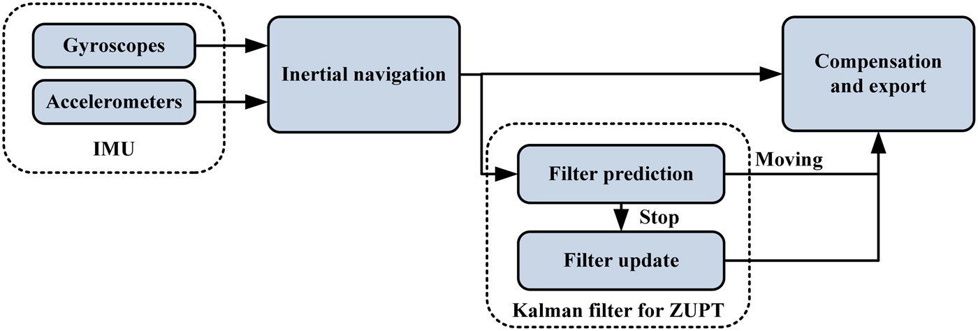
Figure 1. Principle of zero velocity update.
2.2. Strapdown INS Algorithm and Error Model
Most of the land vehicle and pedestrian INSs adopt micromechanical or optical gyroscope strapdown IMUs. In a strapdown INS, the IMU is mounted on the vehicle or the body without a static platform. Angular velocity and acceleration are measured by gyroscopes and accelerometers in the body frame (denoted by b). A mathematical platform is established in the computer to calculate the navigation results (attitude, velocity and position). The local geographical frame (E-N-U frame) is chosen as the navigation frame (denote by n), the strapdown INS algorithm can be written as:
 $$\eqalign{& {\dot{\bi C}}_b^n = {\bi C}_b^n {\bi \Omega} _{nb}^b \cr & {{\dot{\bi v}}}^n = {\bi C}_b^n {\bi f}^b - (2{\bi \omega} _{ie}^n + {\bi \omega} _{en}^n ) \times {\bi v}^n + {\bi g}^n \cr & \dot L = v_N^n \,/\,(R_N + h),\;\dot \lambda = v_E^n \sec L\,/\,(R_E + h),\;{\dot h} = v_U^n} $$
where
 ${\bi \Omega} _{nb}^b = ({\bi \omega} _{nb}^b \times )$
,
${\bi \Omega} _{nb}^b = ({\bi \omega} _{nb}^b \times )$
,
 ${\bi \omega} _{nb}^b = {\bi \omega} _{ib}^b - ({\bi C}_b^n )^T({\bi \omega} _{ie}^n + {\bi \omega} _{en}^n )$
,
${\bi \omega} _{nb}^b = {\bi \omega} _{ib}^b - ({\bi C}_b^n )^T({\bi \omega} _{ie}^n + {\bi \omega} _{en}^n )$
,
 ${\bi g}^n = [0 \quad \ 0\ \quad {-}g ]^T,\ {\bi \omega} _{ie}^n = [0 \quad {\omega _{ie}\cos L}$
 ${\omega _{ie}\sin L} ]^T$
,
${\omega _{ie}\sin L} ]^T$
,
 ${\bi \omega} _{en}^n = [\matrix{ { - v_N^n /(R_N + h)} & {v_E^n /(R_E + h)} & {v_E^n \tan L/(R_E + h)} \cr} ]^T$
.
${\bi \omega} _{en}^n = [\matrix{ { - v_N^n /(R_N + h)} & {v_E^n /(R_E + h)} & {v_E^n \tan L/(R_E + h)} \cr} ]^T$
.
 ${\bi C}_b^n $
is the direction cosine matrix to transform vectors from body frame to navigation frame;
${\bi C}_b^n $
is the direction cosine matrix to transform vectors from body frame to navigation frame;
 ${\bi v}^n$
represents the vector defined by the velocity directions of east, north and up in the navigation frame,
${\bi v}^n$
represents the vector defined by the velocity directions of east, north and up in the navigation frame,
 ${\bi v}^n = [\matrix{ {v_E^n} & {v_N^n} & {v_U^n} \cr} ]^T$
; L, λ and h are the latitude, longitude and height, respectively;
${\bi v}^n = [\matrix{ {v_E^n} & {v_N^n} & {v_U^n} \cr} ]^T$
; L, λ and h are the latitude, longitude and height, respectively;
 ${\bi \omega} _{ib}^b $
represents the angular velocity vector with respect to the inertial space measured by the gyroscope triad in the body frame;
${\bi \omega} _{ib}^b $
represents the angular velocity vector with respect to the inertial space measured by the gyroscope triad in the body frame;
 ${\bi f}^b$
is the specific force vector measured by the accelerometer triad; ω
ie
and g are the self-rotation angular velocity and the gravity acceleration of the earth; R
N
and R
E
are the meridian radius and the transverse radius of curvature, respectively;
${\bi f}^b$
is the specific force vector measured by the accelerometer triad; ω
ie
and g are the self-rotation angular velocity and the gravity acceleration of the earth; R
N
and R
E
are the meridian radius and the transverse radius of curvature, respectively;
 ${\bi \Omega} _{nb}^b $
is the skew symmetric matrix constituted by the element of
${\bi \Omega} _{nb}^b $
is the skew symmetric matrix constituted by the element of
 ${\bi \omega} _{nb}^b = \left[ {\matrix{ {\omega _{nbx}^b} & {\omega _{nby}^b} & {\omega _{nbz}^b} \cr}} \right]^T$
(symbolised by
${\bi \omega} _{nb}^b = \left[ {\matrix{ {\omega _{nbx}^b} & {\omega _{nby}^b} & {\omega _{nbz}^b} \cr}} \right]^T$
(symbolised by
 $({\bi \omega} _{nb}^b \times ) = \left[ {\matrix{ 0 & { - \omega _{nbz}^b} & {\omega _{nby}^b} \cr {\omega _{nbz}^b} & 0 & { - \omega _{nbx}^b} \cr { - \omega _{nby}^b} & {\omega _{nbx}^b} & 0 \cr}} \right]$
in this paper).
$({\bi \omega} _{nb}^b \times ) = \left[ {\matrix{ 0 & { - \omega _{nbz}^b} & {\omega _{nby}^b} \cr {\omega _{nbz}^b} & 0 & { - \omega _{nbx}^b} \cr { - \omega _{nby}^b} & {\omega _{nbx}^b} & 0 \cr}} \right]$
in this paper).
According to the algorithm, the error model of the strapdown INS in Equation (1) can be written as (Titterton and Weston, Reference Titterton and Weston1997):
 $$\eqalign{ {\dot {\bi \psi}} &= - {\bi \psi} \times {\bi \omega} _{in}^n + \delta {\bi \omega} _{in}^n - {\bi C}_b^n \delta {\bi \omega} _{ib}^b \cr \delta {{\dot {\bi v}}}^n &= {\bi f}^n \times {\bi \psi} - (2{\bi \omega} _{ie}^n + {\bi \omega} _{en}^n ) \times \delta {\bi v}^n - (2{\bi \omega} _{ie}^n + {\bi \omega} _{en}^n ) \times {\bi v}^n - \delta {\bi g}^n + {\bi C}_b^n \delta {\bi f}^b \cr \delta \dot L& = \delta v_N^n /(R_N + h) - \delta h \cdot v_N^n /(R_N + h)^2 \cr \delta \dot \lambda & = \delta v_E^n \sec L/(R_E + h) + \delta L \cdot v_E^n \tan L\sec L/(R_E + h) - \delta h \cdot v_E^n \sec L/(R_E + h)^2 \cr \delta \dot h &= \delta v_U^n} $$
where
 $${\bi \omega }_{in}^n = {\bi \omega }_{ie}^n + {\bi \omega }_{en}^n ,\delta {\bi \omega }_{in}^n = \delta {\bi \omega }_{ie}^n + \delta {\bi \omega }_{en}^n ,\delta {\bi \omega }_{ie}^n = [\matrix{ 0 & { - \delta L \cdot \omega _{ie}\sin L} & {\delta L \cdot \omega _{ie}\cos L} \cr } ]^T,$$
 $$\delta {\bi \omega} _{en}^n = \left[ {\matrix{ { - \delta v_N^n /(R_N + h) + \delta h \cdot v_N^n /{(R_N + h)}^2} \cr {\delta v_E^n /(R_E + h) - \delta h \cdot v_E^n /{(R_E + h)}^2} \cr {\delta v_E^n \tan L/(R_E + h) + \delta L \cdot v_E^n {\sec} ^2L/(R_E + h) - \delta h \cdot v_E^n \tan L/{(R_E + h)}^2} \cr}} \right].$$
 ${\bi \psi} $
is the attitude error vector in the mathematical platform,
${\bi \psi} $
is the attitude error vector in the mathematical platform,
 ${\bi \psi} = \left[ {\matrix{ {\delta \alpha} & {\delta \beta} & {\delta \gamma} \cr}} \right]^T$
. δα, δβ and δγ are the three attitude error elements, which can be replaced by the roll, pitch and yaw Euler errors for small angle misalignments;
${\bi \psi} = \left[ {\matrix{ {\delta \alpha} & {\delta \beta} & {\delta \gamma} \cr}} \right]^T$
. δα, δβ and δγ are the three attitude error elements, which can be replaced by the roll, pitch and yaw Euler errors for small angle misalignments;
 $\delta {\bi v}$
is the velocity error vector,
$\delta {\bi v}$
is the velocity error vector,
 $\delta {\bi v} = \left[ {\matrix{ {\delta v_E} & {\delta v_N} & {\delta v_U} \cr}} \right]^T$
. The elements δv
E
, δv
N
and δv
U
denote the velocity errors in the east, north and up direction respectively; δL, δλ and δh stand for the latitude, longitude and height error respectively;
$\delta {\bi v} = \left[ {\matrix{ {\delta v_E} & {\delta v_N} & {\delta v_U} \cr}} \right]^T$
. The elements δv
E
, δv
N
and δv
U
denote the velocity errors in the east, north and up direction respectively; δL, δλ and δh stand for the latitude, longitude and height error respectively;
 $\delta {\bi g}^n$
is the gravity anomaly vector;
$\delta {\bi g}^n$
is the gravity anomaly vector;
 $\delta {\bi \omega} _{ib}^b $
and
$\delta {\bi \omega} _{ib}^b $
and
 $\delta {\bi f}^b$
are the error vectors of gyroscope and accelerometer triad respectively.
$\delta {\bi f}^b$
are the error vectors of gyroscope and accelerometer triad respectively.
2.3. Kalman Filter
In this paper, the attitude errors, velocity errors, position errors, the gyroscope biases (ε
x
, ε
y
and ε
z
) and the accelerometer biases (
 $\nabla _x$
,
$\nabla _x$
,
 $\nabla _y$
and
$\nabla _y$
and
 $\nabla _z$
) are chosen as the state of the Kalman filter:
$\nabla _z$
) are chosen as the state of the Kalman filter:
 $$\eqalign{& {\bi x} = \left[ {\;\delta \alpha \;\;\;\delta \beta \;\;\;\delta \gamma} \right.\;\;\;\delta v_e\;\;\;\delta v_n\;\;\;\delta v_u\;\;\;\delta L\;\;\;\delta \lambda \;\;\;\delta h \cr & \;\;\;\;\;\;\;\varepsilon _x\;\;\;\varepsilon _y\;\;\;\varepsilon _z\;\;\;\nabla _x\;\;\;\nabla _y\;\;\;\nabla _z\left. {} \right]^T} $$
Assuming that the gyroscope and accelerometer measurement errors are constant biases and ignoring the gravity anomaly, the error model can be expressed in a discrete form as:
 $${\bi x}_k = {\bi \Phi} _{k - 1,k}{\bi x}_{k - 1} + {\bi w}_k$$
where
 ${\bi x}_k$
is the state vector at time k;
${\bi x}_k$
is the state vector at time k;
 ${\bi \Phi} _{k - 1,k}$
is the state transition matrix from time k−1 to k;
${\bi \Phi} _{k - 1,k}$
is the state transition matrix from time k−1 to k;
 ${\bi w}_k$
is the system noise.
${\bi w}_k$
is the system noise.
When the vehicle or the body stops, the velocity of the system should be zero in theory. Thus, the observation velocity is expressed as
 ${\bi v}_{obv}^n {\rm = [0}\;\;{\rm 0}\;\;{\rm 0}{\rm ]}^T$
. The measurement equation can be derived as:
${\bi v}_{obv}^n {\rm = [0}\;\;{\rm 0}\;\;{\rm 0}{\rm ]}^T$
. The measurement equation can be derived as:
 $${\bi z}_k = ({\bi v}^n - {\bi v}_{obv}^n ) = {\bi H}_k{\bi x}_k + {\bi v}_k$$
where
 ${\bi z}_k$
is the aiding measurement,
${\bi z}_k$
is the aiding measurement,
 ${\bi H}_k = \left[ {\matrix{ {0_{3 \times 3}} & {{\bi I}_{3 \times 3}} & {0_{3 \times 9}} \cr}} \right]$
is the measurement matrix and
${\bi H}_k = \left[ {\matrix{ {0_{3 \times 3}} & {{\bi I}_{3 \times 3}} & {0_{3 \times 9}} \cr}} \right]$
is the measurement matrix and
 ${\bi v}_k$
is the measurement noise.
${\bi v}_k$
is the measurement noise.
In the Kalman filter, the system and measurement noise are considered as a Gaussian distribution:
 $${\bi w}_k \sim N(0,{\bi Q}_k),\,\,{\bi v}_k \sim N(0,{\bi R}_k)$$
The Kalman filter calculation steps are:
Prediction:
 $${\hat {\bi x}}_{k/k - 1} = {\bi \Phi} _{k - 1,k}{\hat {\bi x}}_{k - 1}$$
 $${\bi P}_{k/k - 1} = {\bi \Phi} _{k - 1,k}{\bi P}_{k - 1}{\bi \Phi} _{k - 1,k}^T + {\bi Q}_k$$
Updating:
 $${\bi K}_k = {\bi P}_{k/k - 1}{\bi H}_k^T [{\bi H}_k{\bi P}_{k/k - 1}{\bi H}_k^T + {\bi R}_k]^{ - 1}$$
 $${\hat {\bi x}}_k = {\hat {\bi x}}_{k/k - 1} + {\bi K}_k[{\bi z}_k - {\bi H}_k{\hat {\bi x}}_{k/k - 1}]$$
 $${\bi P}_k = {\bi P}_{k/k - 1} - {\bi K}_k{\bi H}_k{\bi P}_{k/k - 1}$$
where
 ${\hat {\bi x}}_{k/k - 1}$
and
${\hat {\bi x}}_{k/k - 1}$
and
 ${\bi P}_{k/k - 1}$
are the predicted state and the covariance at time k with the given information at time k−1;
${\bi P}_{k/k - 1}$
are the predicted state and the covariance at time k with the given information at time k−1;
 ${\hat {\bi x}}_{k - 1}$
and
${\hat {\bi x}}_{k - 1}$
and
 ${\bi P}_{k - 1}$
are the estimated state and covariance at time k−1;
${\bi P}_{k - 1}$
are the estimated state and covariance at time k−1;
 ${\hat {\bi x}}_k$
and
${\hat {\bi x}}_k$
and
 ${\bi P}_k$
are the estimated state and covariance at time k.
${\bi P}_k$
are the estimated state and covariance at time k.
3. REVERSE NAVIGATION ALGORITHM
3.1. Discrete Strapdown INS Algorithm
In practice, in order to perform the recursion calculation in a computer, the strapdown INS algorithm in Equation (1) should be discretised:
 $$\eqalign{ {\bi C}_{bk}^n &= {\bi C}_{bk - 1}^n ({\bi I} + T_s{\bi \Omega} _{nbk}^b) \cr {\bi v}_k^n &= {\bi v}_{k - 1}^n + T_s[{\bi C}_{bk - 1}^n{\bi f}_k^b - (2{\bi \omega} _{iek - 1}^n + {\bi \omega} _{enk - 1}^n) \times {\bi v}_{k - 1}^n + {\bi g}^n] \cr L_k &= L_{k - 1} + T_{s}v_{Nk - 1}^n / (R_N + h_{k - 1}) \cr \lambda _k& = \lambda _{k - 1} + T_{s}v_{Ek - 1}^n \sec L_{k - 1} / (R_E + h_{k - 1}) \cr h_k &= h_{k - 1} + T_{s}v_{Uk - 1}^n} $$
where
 $$\matrix{ {{\bi \Omega }{_{nbk}^b } = ({\bi \omega }{_{nbk}^b } \times );} \hfill \cr {{\bi \omega }{_{nbk}^b } = {\bi \omega }{_{ibk}^b } - {({\bi C}{_{bk - 1}^n })}^T({\bi \omega }{_{iek}^n } + {\bi \omega }{_{en}^n });} \cr {{\bi \omega }{_{iek}^n } = {[{\matrix{ 0 & {\omega _{ie}\cos L_k} & {\omega _{ie}\sin L} \cr } }_k]}^T;} \hfill \cr } \quad {\bi \omega }_{enk}^n = \left[ \matrix{ - v_{Nk}^n /(R_N + h_k) \hfill \cr v_{Ek}^n /(R_E + h_k) \hfill \cr v_{Ek}^n \tan L_k/(R_E + h_k) \hfill} \right];$$
k is each discretised time point of the navigation process (k = 1, 2, 3, · · ·).
3.2. Reverse Strapdown INS Algorithm
Assuming that the INS navigates from position A to position B from time t 0 to t, Equation (12) can be transformed to Equation (13) to navigate from position B back to position A reversely (Yan et al., Reference Yan, Yan and Xu2008).
 $$\eqalign{ {\bi C}_{bk - 1}^n &= {\bi C}_{bk}^n ({\bi I} + T_s{\bi \Omega} _{nbk}^b)^{ - 1} \approx {\bi C}_{bk}^n ({\bi I} - T_s{\bi \Omega} _{nbk}^b ) \approx {\bi C}_{bk}^n ({\bi I} + T_s{ \tilde {\bi \Omega}} _{nbk - 1}^b ) \cr {\bi v}_{k - 1}^n & = {\bi v}_k^n - T_s[{\bi C}_{bk - 1}^n{\bi f}_k^b - (2{\bi \omega} _{iek - 1}^n + {\bi \omega} _{enk - 1}^n) \times {\bi v}_{k - 1}^n + {\bi g}^n] \cr & \approx {\bi v}_k^n - T_s[{\bi C}_{bk - 1}^n {\bi f}_{k - 1}^b - (2{\bi \omega} _{iek}^n + {\bi \omega}_{enk}^n) \times {\bi v}_k^n + {\bi g}^n] \cr L_{k - 1} & = L_k - T_{s}v_{Nk - 1}^n/(R_N + h_{k - 1}) \approx L_k - T_{s}v_{Nk}^n /(R_N + h_k) \cr \lambda _{k - 1}& = \lambda _k - T_{s}v_{Ek - 1}^n \sec L_{k - 1}/(R_E + h_{k - 1}) \approx \lambda _k - T_{s}v_{Ek}^n \sec L_k/(R_E + h_k) \cr h_{k - 1} &= h_k - T_{s}v_{Uk - 1}^n \approx h_k - T_{s}v_{Uk}^n} $$
where
 ${ \tilde {\bi \Omega}} _{nbk - 1}^b = ({ \tilde {\bi \Omega}} _{nbk - 1}^b \times )$
;
${ \tilde {\bi \Omega}} _{nbk - 1}^b = ({ \tilde {\bi \Omega}} _{nbk - 1}^b \times )$
;
 ${ \tilde {\bi \Omega}} _{nbk - 1}^b = - [{\bi \omega} _{ib k - 1}^b - ({\bi C}_{bk}^n)^T({\bi \omega} _{iek}^n + {\bi \omega} _{enk}^n )];$
If the reverse velocity is defined as
 ${\bi v}_{rk}^n = - {\bi v}_k^n $
, the reverse strapdown INS algorithm can be written as:
${\bi v}_{rk}^n = - {\bi v}_k^n $
, the reverse strapdown INS algorithm can be written as:
 $$\eqalign{{\bi C}_{bk - 1}^n & = {\bi C}_{bk}^n ({\bi I} + T_s{ \tilde {\bi \Omega}} _{nbrk - 1}^b ) \cr {\bi v}_{rk - 1}^n &= {\bi v}_{rk}^n + T_s[{\bi C}_{bk - 1}^n {\bi f}_{k - 1}^b - ( - 2{\bi \omega} _{iek}^n + {\bi \omega} _{enrk}^n ) \times {\bi v}_{rk}^n + {\bi g}^n] \cr L_{k - 1} &= L_k + T_{s}v_{Nrk}^n /(R_N + h_k) \cr \lambda _{k - 1} &= \lambda _k + T_{s}v_{Erk}^n \sec L_k/(R_E + h_k) \cr h_{k - 1} &= h_k + T_{s}v_{Urk}^n} $$
where
 ${ \tilde {\bi \Omega}} _{nbrk - 1}^b = ({ \tilde {\bi \Omega}} _{nbrk - 1}^b \times )$
;
${ \tilde {\bi \Omega}} _{nbrk - 1}^b = ({ \tilde {\bi \Omega}} _{nbrk - 1}^b \times )$
;
 ${ \tilde {\bi \Omega}} _{nbrk - 1}^b = - {\bi \omega} _{ib {k - 1}}^b - ({\bi C}_{bk}^n)^T( - {\bi \omega} _{iek}^n + {\bi \omega} _{enrk}^n)$
;
${ \tilde {\bi \Omega}} _{nbrk - 1}^b = - {\bi \omega} _{ib {k - 1}}^b - ({\bi C}_{bk}^n)^T( - {\bi \omega} _{iek}^n + {\bi \omega} _{enrk}^n)$
;
 ${\bi \omega} _{enrk}^n = \left[ \matrix{ - v_{Nrk}^n /(R_N + h_k) \hfill \cr v_{Erk}^n /(R_E + h_k) \hfill \cr v_{Erk}^n \tan L_k/(R_E + h_k) \hfill} \right].$
It should be pointed out that, the attitude and position results in the reverse algorithm are the same as those in the forward algorithm, but the velocity result in the reverse algorithm is opposite. Comparing Equation (12) with Equation (14), it can be seen that the reverse algorithm is much the same as the forward algorithm except the sign of gyroscope measurement and self-rotation angular velocity of the earth are opposite. To sum up, the error model of the reverse INS algorithm has a similar form to the model of the forward algorithm except the sign of the gyroscope measurement, the gyroscope bias and the earth rotation angular velocity are opposite.
4. ONLINE SMOOTHING BASED ON REVERSE NAVIGATION
4.1. Principle of Online Smoothing
The principle of the online smoothing based on reverse navigation proposed in this paper is shown in Figure 2. In the forward navigation processing, the Kalman filter for ZUPT is used as usual and the IMU data are stored in the memory. At each time of the navigation process, the reverse navigation algorithm can be performed using the previous IMU data. The initial values of the reverse navigation algorithm are the forward navigation result at this moment. In the reverse navigation algorithm, a reverse Kalman filter for ZUPT is used, which is much the same as the forward one except that the sign of the gyroscope measurement, the gyroscope bias and the earth rotation angular velocity in the state function are opposite. In the reverse navigation algorithm, the fixed-point smoothing method can be used to estimate the navigation errors at the real-time point, while the Rauch-Tung-Striebel (RTS) smoothing can be used to estimate the navigation error of all points in the trajectory including the real-time point. Because the reverse navigation and the smoothing are both reversed processing algorithm, the smoothing in the reverse navigation algorithm turns into forward processing, which can realise online processing in theory and thereby estimate the real-time point or the end point.

Figure 2. Integrated architecture of online smoothing for ZUPT based on reverse navigation.
The process of the online smoothing proposed in this paper is shown in Figure 3. Each line expresses one smoothing calculation process. Taking land vehicle INS for example, the vehicle stops for 10–15 minutes as initial alignment time before navigation. Then, the vehicle also stops for 30–60 seconds for ZUPT after travelling every 8–10 minutes. In the forward navigation algorithm, the Kalman filter performs the updating equation of the Kalman filter (Equations (7) and (8)) by observing the velocity error when the vehicle stops and only carries out the prediction equation of the Kalman filter (Equations (9)–(11)) when the vehicle is travelling. At the same time, the online smoothing proposed in this paper can be performed during the navigation. At each point (normally at the stop point), the reverse navigation (Equation (14)) can be processed using the past IMU data. In the reverse navigation algorithm, when the vehicle is traveling, only the filter prediction step (Equations (7) and (8)) is carried out; when the vehicle stops, the filter updating (Equations (9)–(11)) is carried out by observing the velocity error; when the reverse navigation algorithm is calculated back to the start point, the filter updating is carried out by observing the velocity error and the position error. Then, reversed processing smoothing algorithms such as the RTS smoothing (Equations (18)–(21)) can be carried out in the forward process. Because the position information of the start point is used in the online smoothing algorithm, the position precision can be better than the traditional offline smoothing algorithm.

Figure 3. Process of online smoothing for ZUPT.
4.2. Kalman Smoothing Algorithm
In the online smoothing method proposed in this paper, various Kalman smoothing algorithms can be used. In practice, a suitable smoothing algorithm can be chosen according to the requirement.
4.2.1. Fixed-point smoothing
The fixed-point smoothing is used to estimate the states in a fixed time by all observable information after that time. The calculation steps of fixed-point smoothing are as below.
From the initial time, the updated states
 ${\hat {\bi x}}_k$
and covariance
${\hat {\bi x}}_k$
and covariance
 ${\bi P}_k$
are calculated by the Kalman filter. When the filtering time k is equal to or later than the smoothing time j, the state vector at the smoothing time can be estimated by the iterative equation after the Kalman filter:
${\bi P}_k$
are calculated by the Kalman filter. When the filtering time k is equal to or later than the smoothing time j, the state vector at the smoothing time can be estimated by the iterative equation after the Kalman filter:
 $${\hat {\bi x}}_{\,j/k} = {\hat {\bi x}}_{\,j/k - 1} + {\bi K}_k^a ({\bi z}_k - {\bi H}_k{\hat {\bi x}}_{k/k - 1})$$
 $${\bi K}_k^a = {\bi P}_{k/k - 1}^a {\bi H}_k^T ({\bi H}_k{\bi P}_{k/k - 1}{\bi H}_k^T + {\bi R}_k)^{ - 1}$$
The iterative equation of covariance matrix
 ${\bi P}_{k + 1/k}^a $
in the fixed-point smoother can be presented as:
${\bi P}_{k + 1/k}^a $
in the fixed-point smoother can be presented as:
 $${\bi P}_{k + 1/k}^a = {\bi P}_{k/k - 1}^a {\bi} \left( {{\bi \Phi} _{k + 1,k}{\bi -} {\bi \Phi} _{k + 1,k}{\bi {\rm K}}_k{\bi H}_k^T} \right)^T$$
Because the fixed-point smoothing does not need to store the filtering information, it has a low requirement of the computer's speed and storage space, which applies to the online smoothing, but only one point can be estimated in each smoothing operation.
4.2.2. RTS smoothing
The RTS smoothing is also called fixed-interval smoothing, which can estimate the states in the whole trajectory using discontinuous observable information (Gong et al., Reference Gong, Zhang and Fang2013; Liu et al., Reference Liu, Nassar and El-Sheimy2010). The calculation steps of the RTS smoother are as below.
While the Kalman filter is working, the predicted states
 ${\hat {\bi x}}_{k/k - 1}$
and covariance
${\hat {\bi x}}_{k/k - 1}$
and covariance
 ${\bi P}_{k/k - 1}$
, the updated states
${\bi P}_{k/k - 1}$
, the updated states
 ${\hat {\bi x}}_k$
and covariance
${\hat {\bi x}}_k$
and covariance
 ${\bi P}_k$
are all stored in memory for smoothing later. We assume that there are M times in the whole trajectory, and each time can be denoted as j (0 < j < M). After the calculation of the Kalman filter, the RTS smoother begins at time M. With j = M, M − 1, · · · , 1, the iterative equation of the state vector in the RTS smoother can be written as:
${\bi P}_k$
are all stored in memory for smoothing later. We assume that there are M times in the whole trajectory, and each time can be denoted as j (0 < j < M). After the calculation of the Kalman filter, the RTS smoother begins at time M. With j = M, M − 1, · · · , 1, the iterative equation of the state vector in the RTS smoother can be written as:
 $${\hat {\bi x}}_{\,j - 1/M} = {\hat {\bi x}}_{\,j - 1} + {\bi A}_{\,j - 1}\left( {{{\hat {\bi x}}}_{\,j/M} - {{\hat {\bi x}}}_{\,j/j - 1}} \right)$$
 $${\bi A}_{\,j - 1} = {\bi P}_{\,j - 1}{\bi \Phi} _{\,j,j - 1}^T {\bi P}_{\,j/j - 1}^{ - 1} $$
The iterative equation of the covariance matrix in the RTS smoother can be presented as:
 $${\bi P}_{\,j - 1/M} = {\bi P}_{\,j - 1} + {\bi A}_{\,j - 1}{\bi} \left( {{\bi P}_{\,j/M}{\bi -} {\bi P}_{\,j/j - 1}} \right){\bi A}_{\,j - 1}^T $$
where the updated states and covariance at time M of the Kalman filter is the initial value of the RTS smoother.
 $${\hat {\bi x}}_{M/M}{\bi = }{\hat {\bi x}}_M\,{\bi P}_{M/M} = {\bi P}_M$$
In this paper, the RTS smoothing is chosen to perform a high-accuracy estimation of the navigation errors. It should be pointed out that because the RTS smoothing has to store the filtering information during the navigation, it has a relatively high requirement of the computer's processing speed and storage space. To improve the software for making the online smoothing algorithm applicable to common hardware, the calculation frequency of the smoothing process can be reduced from 100 Hz to 1 Hz or even lower. In this way, only the averaged data for each second needs to be stored, and the storage space and the processing speed required of the computer can be reduced to 1% or lower.
5. FIELD TESTS
5.1. Test Arrangement
Field navigation tests were carried out in Changsha to verify the effectiveness of the online smoothing method for ZUPT-aided INS. Two IMUs with the same level of accuracy were used in the tests. Both IMUs consisted of three Ring Laser Gyros with an accuracy of 0·003°/h and three quartz accelerometers with an accuracy of 10 µg. An indexing mechanism with an accuracy of 5″ was used for estimating the inertial sensor biases during the alignment. The sampling frequency was 100 Hz. A Differential GPS (DGPS) with an accuracy of 3 cm was used to provide the reference position information for comparison. The test car, the DGPS base station and the installation of the IMU on the indexing mechanism and on the vehicle are shown in Figure 4.

Figure 4. Field test facilities.
To verify the method used in different IMUs, paths and stop intervals, six navigation tests (listed in Table 1) were designed.
Table 1. Introduction of the navigation tests.

5.2. Accuracy Test Results
In the first two tests, IMU1 was used to navigate for 2 h and 1 h 50 min respectively. During the alignment, the azimuth axis of the IMU was turned 90° by the indexing mechanism to estimate and compensate the biases of the inertial sensors. During the navigation, the test car stopped for 30 s every 10 min for ZUPT. The navigation results of Test 1 and Test 2 are shown in Figures 5 and 6. In each figure, the navigation trajectory is shown in Figure (a), the errors of inertial navigation without ZUPT are shown in Figure (b), the errors with traditional ZUPT mentioned in Section 2 are shown in Figure (c) and the errors with online smoothing ZUPT proposed in this paper are shown in Figure (d), respectively. We can see from the figures that the max position error of inertial navigation without ZUPT is about 500 m over 2 h. The position error at stop points can be compensated to 5·5 m by ZUPT-aiding, but when the car was running, the position error accumulated to 15 m in 10 min. With the online smoothing ZUPT-aiding, the maximum position error during the whole trajectory was restrained to below 5 m in both tests. It has to be pointed out that the unconventional points such as the 20 m error in Figure 6(c) and Figure 6(d) are caused by a break in the DGPS signal when the car traversed through bridges and other obstructions. That is also the reason why the position error at Stop point 5 in Test 2 cannot be obtained.

Figure 5. Results of Test 1.

Figure 6. Results of Test 2.
In Test 3 and Test 4 the method is verified using a different IMU (IMU2). Each test lasted for 1 h 20 min, and the test car also stopped for 30 s every 10 min for ZUPT. In Test 3, the biases of the inertial sensors were also estimated and compensated by the indexing mechanism, and the path was also random as in Test 1 and Test 2. The navigation result is similar to the first two tests as shown in Figure 7. The maximum position error at the stop points was decreased to 4·6 m by ZUPT-aiding, and during the whole trajectory was restrained to 4·3 m by the online smoothing ZUPT-aiding. It further illustrates the efficiency of the online smoothing method on high-accuracy IMU.

Figure 7. Results of Test 3.
The position errors in Test 4 are larger than those in the previous three tests, especially at the third stop point, which is twice as large as the max error in the previous tests. This is because during the alignment and the navigation before the third stop point, the orientation of the IMU had not changed. Under this condition, the horizontal attitude angle errors are coupled with the accelerometer bias as well as the azimuth error and the gyro bias, and therefore some states of the Kalman filter cannot be convergent. After the vehicle turned 180°, the errors were decoupled and all states of the Kalman filter were convergent so that all the errors were estimated at the next stop point by observing the velocity error. Thus the position error was restrained after the fifth stop point. We can infer from the result that turning of the vehicle is necessary for a ZUPT-aiding INS to improve the observability and ensure the Kalman filter is convergent. According to the test result, the issue of low observability in straight trajectory can be solved by adding a single-axis indexing mechanism. The errors can be decoupled by only one 90° rotation around the azimuth axis during alignment with no need of rotation during navigation. In addition, it can be seen by comparing Figure 8(c) with Figure 8(d) that the online smoothing algorithm can clearly improve the accuracy of ZUPT under bad observability conditions as well.

Figure 8. Results of Test 4.
The test conditions in Test 5 and Test 6 were the same as in Test 3, except the stop interval was extended to 15 min. Test results are shown in Figure 9 and Figure 10. The maximum position error at stop points was compensated to 8·7 m by ZUPT-aiding, and during the whole trajectory it was restrained from 70 m to 14·4 m by the online smoothing ZUPT-aiding in both tests. This proves that the online smoothing ZUPT method can maintain a high accuracy estimation even if the observation interval is extended to 15 min.

Figure 9. Results of Test 5.

Figure 10. Results of Test 6.
Statistical results of the six tests are shown in Table 2. When the stop interval is 10 min, the max position error at the stop points is 5·5 m by ZUPT-aiding, and it is 4·9 m during the whole trajectory by online smoothing ZUPT-aiding except the unusual points in Test 4. When the stop interval extends to 15 min, the max position error at the stop points was 8·7 m by ZUPT-aiding, and it was 14·4 m during the whole trajectory by the online smoothing ZUPT-aiding. This proves that by using the proposed online smoothing ZUPT method, the position error in the whole trajectory can be restrained to the same level of those at the stop points. The test results reach quite a high level accuracy in a state-of-art technical condition, which verifies the advancement of online smoothing ZUPT method proposed in this paper.
Table 2. Statistical Results of the Six Tests.

5.3. Delay Test Results
A delay test with a calculation frequency of 1 Hz was designed for calculating the position accuracy and the delay time of the reverse online smoothing method proposed in this paper. A commonly used computer with a 4 GHz quad-core processor and a 120 GB solid-state drive is adopted in the test. The 100 Hz gyro and accelerometer data of Test 1 is read for each 10 ms to simulate the online condition and the delay time is recorded by computer. The test results of existing step-wise online smoothing method and the reverse online smoothing method proposed in this paper are shown in Figure 11. It can be seen from Figure 11(a), that the accuracy of the two smoothing methods are similar and the accuracy with 1 Hz smoothing is no worse than the accuracy of Test 1 in Figure 5. It can be seen from Figure 11(b), limited by the principle, that the step-wise online smoothing method can process a step of smoothing only when the observation is obtained. The largest delay time is about 10 min because the vehicle stops every 10 min. The theoretical delay of the proposed reverse online smoothing method is 1 s because the smoothing calculation frequency is 1 Hz. In practice, this is limited by the computer's calculation speed, and the delay time increases with navigation time because the data size accumulates. However, the delay is no more than 3 s after 1 h navigation and no more than 20 s after 2 h navigation using a common computer, which is much shorter than that with the traditional online smoothing method.

Figure 11. Results of delay test results.
6. CONCLUSION AND DISCUSSION
Smoothing methods in ZUPT-aided navigation can effectively restrain position errors not only at stop points but also during the whole trajectory in independent navigation systems. To realise real-time high-accuracy estimation, an online smoothing method for ZUPT-aided INS based on reverse navigation is proposed in this paper. Six tests with two different IMUs are designed to verify the effectiveness of the proposed method. The online smoothing method was performed in different trajectories with different stop intervals. Test results prove that the online smoothing method with ZUPT can improve the position accuracy during the whole trajectory, including at real time points and the end point, to the level nearly equivalent to the accuracy at the stop points, and the results can be even better when the stop interval is reduced to 10 min or shorter. In the delay test result, the delay is no more than 3 s and 20 s after 1 h and 2 h navigation using a common computer, respectively. This is much shorter than the traditional online smoothing method. The results reach a quite a high level of accuracy in a state-of-art technical condition, which verifies the advancement of the online smoothing ZUPT method proposed in this paper.
The proposed online smoothing method has shown a great potential in land vehicle navigation for the rapidly rising Vehicle Networking and self-driving technology, which can provide high accuracy position and attitude of vehicles in real time in an urban-canyon environment. The method researched in this paper is also helpful to improve the adaptability of ZUPT-aided pedestrian INSs in flexible walking motion conditions, such as while running. In the future, the proposed online smoothing method will be verified in a Micro-Electromechanical Systems (MEMS) pedestrian navigation system.


