2.1 Quaternion-based EKF system

EKF is widely used for nonlinear systems and long-running processes (Poulose et al., Reference Poulose, Senouci and Han2019). Further, quaternion is used to describe the attitude information, because of its superiority of no singularity problem and higher computation efficiency than Euler angles (Yuan et al., Reference Yuan, Yu, Zhang, Wang and Liu2015).

Using normalised rotation quaternion, the heading estimation as a state vector at time stamp k is represented by

(2.1)\begin{equation}{\boldsymbol{X}_{\boldsymbol{k}}} = \left[ \begin{matrix}{q_k^0}&{q_k^1} & {q_k^2}&{q_k^3} \end{matrix}\right]^{\rm T}\end{equation}

where $q_k^0$ denotes the scalar part, and ${\left[ {\begin{array}{*{20}{c}} {q_k^1}&{q_k^2}&{q_k^3} \end{array}} \right]^{\rm T}}$ denotes the vector part.

According to the quaternion attitude kinematics equations (Oshman and Carmi, Reference Oshman and Carmi2006), we can deduce the discrete time model as

(2.2)\begin{equation} {{\boldsymbol{X}_{\boldsymbol{k}}} = \left( {I + \dfrac{T}{2} \cdot {\mathbf{\Omega}}_{\boldsymbol{k} - 1}^{\boldsymbol{b}}} \right) \cdot {\boldsymbol{X}_{\boldsymbol{k} - 1}}} \end{equation}

where T = sensors sampling interval, ${\mathbf{I}}$ = $4 \times 4$ identity matrix, and ${\mathbf{\Omega}}_{\boldsymbol{k}}^{\boldsymbol{b}}$ is constructed by

(2.3)\begin{equation} {\mathbf{\Omega}}_k^b = \left[\begin{matrix} 0 & - \omega_k^{x} & - \omega_k^{y} & - \omega_k^{z}\\ \omega_k^{x} & 0 & \omega_k^{z} & \omega_k^{y} \\ \omega_k^{y} & - \omega_k^{z} & 0 & \omega_k^{x}\\ \omega_k^{z} & \omega_k^{y} & -\omega_k^{x} & 0 \end{matrix}\right] \end{equation}

Observations are formed by the pitch angle ${\theta _k}$, roll angle ${\phi _k}$, and yaw ${\psi _k}$, which can be calculated by accelerations and magnetic field. Thus, the quaternion form of the Euler angles is given as

(2.4)\begin{equation} {\boldsymbol{Z}_{\boldsymbol{k}}} = \left[ \begin{matrix} {{q_0}}\\ {{q_1}} \\ {{q_2}}\\ {{q_3}} \end{matrix} \right] = \left[\begin{matrix} {\cos \dfrac{\phi }{2}\cos \dfrac{\theta }{2}\cos \dfrac{\psi }{2} + \sin \dfrac{\phi }{2}\sin \dfrac{\theta }{2}\sin \dfrac{\psi }{2}}\\ {\sin \dfrac{\phi }{2}\cos \dfrac{\theta }{2}\cos \dfrac{\psi }{2} - \cos \dfrac{\phi }{2}\sin \dfrac{\theta }{2}\sin \dfrac{\psi }{2}} \\ {\cos \dfrac{\phi }{2}\sin \dfrac{\theta }{2}\cos \dfrac{\psi }{2} + \sin \dfrac{\phi }{2}\cos \dfrac{\theta }{2}\sin \dfrac{\psi }{2}}\\ {\cos \dfrac{\phi }{2}\cos \dfrac{\theta }{2}\sin \dfrac{\psi }{2} - \sin \dfrac{\phi }{2}\sin \dfrac{\theta }{2}\cos \dfrac{\psi }{2}} \end{matrix}\right] \end{equation}

Considering a nonlinear discrete EKF system as

(2.5)\begin{equation}\begin{cases} {{\boldsymbol{X}_{\boldsymbol{k}}} = {{\mathbf{\Phi} }_{\boldsymbol{k},\boldsymbol{k} - 1}}({{\boldsymbol{X}_{\boldsymbol{k} - 1}},k - 1} )+ {\boldsymbol{w}_{\boldsymbol{k} - 1}}}\\ {{\boldsymbol{Z}_{\boldsymbol{k}}} = h({{\boldsymbol{X}_{\boldsymbol{k}}},k} )+ {\boldsymbol{v}_{\boldsymbol{k} - 1}}}\end{cases} \end{equation}

where ${\boldsymbol{Z}_{\boldsymbol{k}}}$ = observation of system, and ${\boldsymbol{w}_{\boldsymbol{k}}}$ and ${\boldsymbol{v}_{\boldsymbol{k}}}$ = process noise vector with covariance matrix ${{\mathbf{Q}}_{\mathbf{k}}} = \sigma _q^2 \cdot {\mathbf{I}}$ and measurement noise vector with covariance matrix ${{\mathbf{R}}_{\mathbf{k}}} = \sigma _R^2 \cdot {\mathbf{I}}$.

The state transition matrix is

(2.6)\begin{equation} {{\mathbf{\Phi} }_{\boldsymbol{k},\boldsymbol{k} - 1}} = I + \dfrac{T}{2} \cdot \left[ \begin{matrix} 0 & { - \omega_k^x} &{ - \omega_k^y} & { - \omega_k^z}\\ {\omega_k^x} &0 &{\omega_k^z} &{\omega_k^y} \\ {\omega_k^y} & { - \omega_k^z} &0 &{\omega_k^x}\\ {\omega_k^z} & {\omega_k^y} & { - \omega_k^x} & 0 \end{matrix}\right] \end{equation}

The measurement matrix ${{\mathbf{H}}_{\mathbf{k}}}$ is an $4 \times 4$ identity matrix for the linear measurement equation.

Finally, the heading estimation $\hat{\psi }$ from the EKF model is given by

(2.7)\begin{equation}\begin{array}{*{20}{c}} {\hat{\psi }\; = \; {{\tan }^{ - 1}}\left[ {\dfrac{{2({{q_0}{q_3} + {q_1}{q_2}} )}}{{1 - 2({q_2^2 + q_3^2} )}}} \right]} \end{array}\end{equation}

2.2 DTW-based straight-walk detection

There are mainly two pedestrian motion patterns in common indoor environments with regular corridors and corners, such as schools and supermarkets. One pattern is walking straight with a stable heading, such as along a corridor. Another pattern is turning with an apparent heading change at a short time, such as at a corner. However, due to the low quality of the sensors in smartphones, the heading estimation of the EKF system will gradually deviate from the truth, even when the user is walking straight ahead. Given that indoor moving activities involve mostly straight-line walking and less time in turning (Borenstein and Ojeda, Reference Borenstein and Ojeda2010), we proposed an accurate straight walk to limiting the heading estimation, which should be unchanged.

While holding a smartphone in front of the body, the z-axis gyro measurements present periodic feature, and shown as Figure 2.

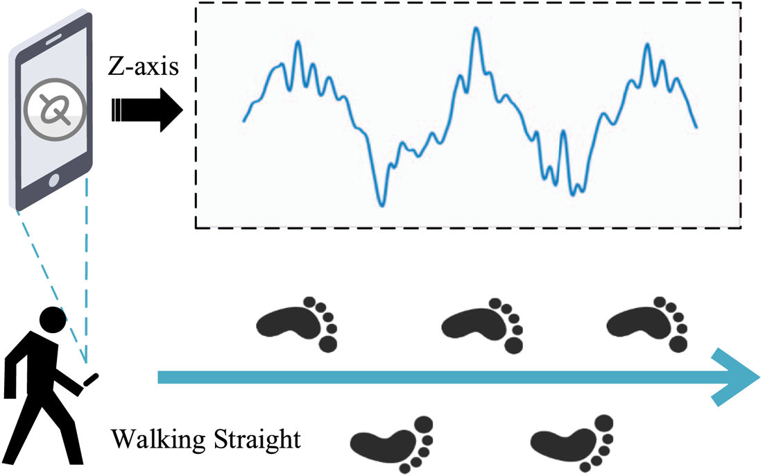
Figure 2. Periodicity of gyro measurement while walking straight

We employ the DTW method to calculate the shortest distance of z-axis part of angular velocity, within the adaptive window size N from the time interval of steps. Let $trj_{k}$ represents the sample point of a trajectory z-axis gyro measurements set at time stamp k. The shortest distance $D_{k}$ is used as dissimilarity between current sample point set $\boldsymbol{seg}_{1,\boldsymbol{k}}$ and previous one $\boldsymbol{seg}_{0,\boldsymbol{k}}$, which are given by

(2.8)\begin{equation}\left\{ \begin{array}{l} \boldsymbol{seg}_{0,\boldsymbol{k}} = [trj_{k - 2N + 1},trj_{k - 2N + 2}, \cdots ,trj_{k - N} ]\\ \boldsymbol{seg}_{1,\boldsymbol{k}} = [{trj_{k - N + 1},trj_{k - N + 1}, \cdots ,trj_k}]\\ {D_k} = DTW(\boldsymbol{seg}_{0,\boldsymbol{k}},\boldsymbol{seg}_{1,\boldsymbol{k}} )\end{array} \right.\end{equation}

According to the dissimilarity, we build a threshold-based state machine to recognise the motion patterns. A typical pedestrian trajectory is selected to illustrate the DTW-based straight-walk detection method. It includes standing still, walking straight for several steps and a ninety-degree turning. Figure 3 shows the state machine, z-axis component of gyro measurements and their corresponding dissimilarity.

Figure 3. (a) The state machine. (b) Z-axis component of gyro measurements. (c) Corresponding DTW results

The several thresholds are suffixed with ‘$\_\textrm{Thr}$’, and the six states are explained as follows:

1. 1) S1: Static state. ${D_k} < \textrm{Static}\_\textrm{Thr}$. The initial state is always S1, and means the pedestrian has no movement. While ${D_k} > \textrm{Static}\_\textrm{Thr}$, the current state becomes S2.

2. 2) S2: Transition state between S1 and S3. ${D_k} < \textrm{Turn}\_\textrm{Thr}$. In this state, the pedestrian begins to move, but may be walking straight or turning. The increment of ${D_k}$ is set as

   (2.9)\begin{equation}\begin{array}{*{20}{c}} {\Delta {D_k} = {D_k} - {D_{k - 1}}} \end{array}\end{equation}
   While ${D_k} < \textrm{Straight}\_\textrm{Thr}$ and $\Delta {D_k} < 0$, the state becomes S3. And while ${D_k} > \textrm{Turn}\_\textrm{Thr}$, the state becomes S5.

3. 3) S3: Straight state. ${D_k} < \textrm{Straight}\_\textrm{Thr}$. This state means the user is walking straight and keeping a stable heading angle. Thus, during this state, pseudo-gyro measurements $\boldsymbol{w}_{\boldsymbol{k}}^{\boldsymbol{p}}$ and the state transition matrix ${{\mathbf{\Phi} }_{\boldsymbol{k},\boldsymbol{k} - 1}}$ of EKF are provided as

   (2.10)\begin{align}\boldsymbol{w}_{\boldsymbol{k}}^{\boldsymbol{p}} &= \beta \cdot {\boldsymbol{w}_{\boldsymbol{k}}} = \beta \cdot \left[ {\begin{matrix} {\omega_k^x}&{\omega_k^y}&{\omega_k^z} \end{matrix}} \right] \end{align}
   (2.11)\begin{align} {\mathbf{\Phi}}_{\boldsymbol{k},\boldsymbol{k} - 1} &= I + \frac{{\mathrm{\beta }T}}{2} \cdot \left[ \begin{matrix} 0 & { - \omega_k^x} & { - \omega_k^y} & { - \omega_k^z}\\ {\omega_k^x} &0 &{\omega_k^z} &{\omega_k^y}\\ {\omega_k^y} & { - \omega_k^z} & 0 & {\omega_k^x}\\ {\omega_k^z} & {\omega_k^y} &{ - \omega_k^x} & 0 \end{matrix}\right]\end{align}
   where $0 < \beta < 1$ is the constraint parameter and ${w_k}$ = raw gyro measurements. While ${D_k} > \textrm{Straight}\_\textrm{Thr}$, the state becomes S4.

4. 4) S4: Transition state between S3 and S5. ${D_k} < \textrm{Turn}\_\textrm{Thr}$. This state means that the pedestrian may begin turning or is stopped. While ${D_k} < \textrm{Straight}\_\textrm{Thr}$ again, the state becomes S1. During this state, while ${D_k} > \textrm{Turn}\_\textrm{Thr}$, the state becomes S5 and in the meantime the heading difference $\delta \psi$ between magnetic-based observation ${\psi _k}$ and EKF-based state estimation ${\hat{\psi }_k}$ is recorded and will be used for compensating the heading error due to time delay of state transition, as

   (2.12)\begin{equation}\begin{array}{*{20}{c}} {\delta \psi = {\psi _k} - \; {{\hat{\psi }}_k}} \end{array}\end{equation}

5. 5) S5: Turning state. As soon as this state is detected, the real gyro measurements must be applied to track the heading change, and $\delta \psi$ is used for feedback correction, as shown in Figure 4.

6. 6) S6: Transition state between S5 and S3. It means the end of a turn and while ${D_k} < \textrm{Straight}\_\textrm{Thr}$, the state becomes S3.

Figure 4. Feedback correction of heading estimation

By applying straight-walk detection in pedestrian tracking, we not only limit the inherent heading deviation caused by the built-in sensors in the mobile phones, but also can constrain the irregular heading fluctuation caused by the swing of pedestrians.

2.3 Joint quasi static field detection

Due to hard iron error and soft iron error, magnetometer should be calibrated first. We use smartphones to collect magnetic field data in all directions in the same location and, finally, these data point will form an ellipsoid in three-dimensional space. Hence, the calibration problem can be solved by calculating the parameter of the ellipsoid, just as

(2.13)\begin{equation}\begin{array}{*{20}{c}} {\begin{array}{*{20}{c}} {1 = {a_1}{x^2} + {a_2}{y^2} + {a_3}{z^2} + {a_4}xy + {a_5}xz + {a_6}yz + {a_7}x + {a_8}y + {a_9}z} \end{array}} \end{array}\end{equation}

where ($x,y,z$) = collected data point of three-axis magnetometer, and (2.12) can be described by matrix as

(2.14)\begin{equation}\begin{array}{*{20}{c}} {\left[ {\begin{array}{*{20}{c}} {\begin{array}{*{20}{c}} 1\\ 1 \end{array}}\\ \vdots \\ 1 \end{array}} \right] = \left[ {\begin{array}{*{20}{c}} {\begin{array}{*{20}{c}} {\begin{array}{*{20}{c}} {x_1^2}&{y_1^2}&{z_1^2} \end{array}}\\ {\begin{array}{*{20}{c}} {x_2^2}&{y_2^2}&{z_2^2} \end{array}} \end{array}}& \cdots &{\begin{array}{*{20}{c}} {\begin{array}{*{20}{c}} {{x_1}}&{{y_1}}&{{z_1}} \end{array}}\\ {\begin{array}{*{20}{c}} {{x_2}}&{{y_2}}&{{z_2}} \end{array}} \end{array}}\\ \vdots & \ddots & \vdots \\ {\begin{array}{*{20}{c}} {x_n^2}&{y_n^2}&{z_n^2} \end{array}}& \cdots &{\begin{array}{*{20}{c}} {{x_n}}&{{y_n}}&{{z_n}} \end{array}} \end{array}} \right]\left[ {\begin{array}{*{20}{c}} {\begin{array}{*{20}{c}} {{a_1}}\\ {{a_2}} \end{array}}\\ \vdots \\ {{a_9}} \end{array}} \right]} \end{array}\end{equation}

that is simplified as

(2.15)\begin{equation}\mathbf{I} = \textbf{HX}\end{equation}

Thus, the three-axis scale factors and bias factors can be calculated as

(2.16)\begin{equation} X = \left[ \begin{matrix} a_1\\ a_2 \\ \vdots \\ a_9 \end{matrix} \right] = (\textbf{H}^{\textbf{T}}\textbf{H})^{ - 1}\textbf{H}^{\textbf{T}}I \end{equation}

In addition, indoor magnetic field disturbance can also cause deviation from the true local magnetic field. Fusing these bad magnetic measurements will certainly bring additional estimation error. Afzal et al. (Reference Afzal, Renaudin and Lachapelle2011), proposed a QSF detector to identify the quasi-static magnetic field based on the change of the total magnetic induction strength. However, there exist several situations in which the heading observation change sharply with a small change in the total magnetic induction strength.

In this paper, we also consider the change of the heading value computed by magnetic and the difference of heading value between current state prediction of EKF and magnetic-based method, as the additional QSF detectors.

At time stamp k, we assume that the heading value computed by magnetic field is ${\varphi _k}$, the difference between the prediction of EKF and ${\varphi _k}$, is ${\gamma _k}$, and the total magnetic induction strength is $||{ {{B_k}} ||}$. Then the observation model of JQSF is constructed by

(2.17)\begin{equation}\begin{array}{*{20}{c}} {{\boldsymbol{y}_{\boldsymbol{k}}} = {\boldsymbol{s}_{\boldsymbol{k}}} + {\boldsymbol{v}_{\boldsymbol{k}}}} \end{array}\end{equation}

where ${\boldsymbol{y}_{\boldsymbol{k}}}$ = observation, ${\boldsymbol{s}_{\boldsymbol{k}}} = {\left[ {\begin{array}{*{20}{c}} {s_k^\gamma }&{s_k^\varphi }&{s_k^B} \end{array}} \right]^\textrm{T}}$, $s_k^\gamma = {\gamma _k}$,$\; s_k^\varphi = {\varphi _k} - {\varphi _{k - 1}}$, $s_k^B = ||{ {{B_k}} ||} - ||{ {{B_{k - 1}}} ||}$ and ${\boldsymbol{v}_{\boldsymbol{k}}} = {\left[ {\begin{array}{*{20}{c}} {v_k^\gamma }&{v_k^\varphi }&{v_k^B} \end{array}} \right]^\textrm{T}}$ = Gaussian white noises with zero means, which are independent and identically distributed as

(2.18)\begin{equation}\begin{array}{*{20}{c}} {E[{{\boldsymbol{v}_{\boldsymbol{k}}}\boldsymbol{v}_{\boldsymbol{k}}^{\mathbf{T}}} ]= \left[ {\begin{array}{*{20}{c}} {\sigma_\gamma^2}&0&0\\ 0&{\sigma_\varphi^2}&0\\ 0&0&{\sigma_B^2} \end{array}} \right]} \end{array}\end{equation}

where $\sigma _\gamma ^2$, $\sigma _\varphi ^2$ and $\sigma _B^2$ = corresponding variance of $s_k^\gamma$,$\; s_k^\varphi$ and $s_k^B$. The optimal set of the variance can be determined by fine-tuning the statistical results from the measured data.

During the straight-walk state, for a window size N, if there exists a quasi-static magnetic field, the heading value from magnetic field should remain unchanged, as well as the total field strength, that is $s_k^\varphi = 0$ and $s_k^B = 0$. If one of $s_k^\varphi$ and $s_k^B$ is non-zero, there may exist a nonstatic field. Thus, we assume that the hypothesis of a nonstatic field is ${H_0}$ and that for a quasi-static field is ${H_1}$, which are given as

(2.19)\begin{equation}\begin{array}{*{20}{c}} {\left\{ {\begin{array}{*{20}{c}} {{H_0}:\; \exists k \in {\boldsymbol{\Omega }_{\boldsymbol{n}}},\; ({s_k^\varphi \ne 0} )\vee ({s_k^B \ne 0} )}\\ {{H_1}:\; \forall k \in {\boldsymbol{\Omega }_{\boldsymbol{n}}}, \; ({s_k^\varphi = 0} )\wedge ({s_k^B \ne 0} )} \end{array}} \right.} \end{array}\end{equation}

where ${\boldsymbol{\Omega }_{\boldsymbol{n}}} = \{{j \in N:\; n \le j \le n + N - 1} \}$ and n = step number.

We use the maximum likelihood estimator (MLE) to estimate the unknown parameter ${\boldsymbol{s}_{\boldsymbol{k}}}$ in the case of ${H_0}$, giving

(2.20)\begin{equation}\begin{array}{*{20}{c}} {\left\{ {\begin{array}{*{20}{c}} {\hat{s}_k^\varphi = \dfrac{1}{N}\sum\limits_{k \in {\Omega _n}} {y_k^\varphi } }\\ {\hat{s}_k^B = \dfrac{1}{N}\sum\limits_{k \in {\Omega _n}} {y_k^B} } \end{array}} \right.} \end{array}\end{equation}

where $\hat{s}_k^\varphi$ and $\hat{s}_k^B$ = MLE result of $s_k^\varphi$ and $s_k^B$ under ${H_0}$.

Then, the probability density functions (PDFs) under two cases can be given by

(2.21)\begin{align}&\left\{ {\begin{array}{*{20}{c}} {f({\boldsymbol{y};[{s_k^\varphi \; s_k^B} ],\; {H_0}} )= \mathop \prod \limits_{k \in {\Omega _n}} f({{\boldsymbol{y}_{\boldsymbol{k}}};s_k^\varphi ,{H_0}} )\cdot f({{\boldsymbol{y}_{\boldsymbol{k}}};s_k^B,{H_0}} )}\\ {f({y_k^\varphi ;s_k^\varphi ,{H_0}} )= \dfrac{1}{{2\pi \sigma_\varphi^2}}\exp\left( { - \dfrac{1}{{2\sigma_\varphi^2}}{{({y_k^\varphi - \hat{s}_k^\varphi } )}^2}} \right)}\\ {f({y_k^B;s_k^B,{H_0}} )= \dfrac{1}{{2\pi \sigma_B^2}}\exp\left( { - \dfrac{1}{{2\sigma_B^2}}{{({y_k^B - \hat{s}_k^B} )}^2}} \right)} \end{array}} \right.\end{align}

(2.22)\begin{align}&\left\{ {\begin{array}{*{20}{c}} {f({\boldsymbol{y};[{s_k^\varphi \; s_k^B} ],\; {H_1}} )= \mathop \prod \limits_{k \in {\Omega _n}} f({{\boldsymbol{y}_{\boldsymbol{k}}};s_k^\varphi ,{H_1}} )\cdot f({{\boldsymbol{y}_{\boldsymbol{k}}};s_k^B,{H_1}} )}\\ {f({y_k^\varphi ;s_k^\varphi ,{H_1}} )= \dfrac{1}{{2\pi \sigma_\varphi^2}}\exp\left( { - \dfrac{1}{{2\sigma_\varphi^2}}{{({y_k^\varphi } )}^2}} \right)}\\ {f({y_k^B;s_k^B,{H_1}} )= \dfrac{1}{{2\pi \sigma_B^2}}\exp\left( { - \dfrac{1}{{2\sigma_B^2}}{{({y_k^B} )}^2}} \right)} \end{array}} \right.\end{align}

The generalised likelihood ratio test (GLRT) is used for detecting a quasi-static magnetic field during the straight-walk state, as

(2.23)\begin{equation}\dfrac{{f({\boldsymbol{y};[{s_k^\varphi \; s_k^B} ],\; {H_0}} )}}{{f({\boldsymbol{y};[{s_k^\varphi \; s_k^B} ],\; {H_1}} )}} < \lambda\end{equation}

where $\mathrm{\lambda }$ = threshold for GLRT, for (2.20) and (2.21) in (2.22), and taking the natural log function on both sides and simplifying as

(2.24)\begin{equation}\dfrac{1}{N}\left( {\dfrac{1}{{\sigma_\varphi^2}}{{\left( {\sum\limits_{k \in {\boldsymbol{\Omega }_{\boldsymbol{n}}}} {y_k^\varphi } } \right)}^2} + \dfrac{1}{{\sigma_B^2}}{{\left( {\sum\limits_{k \in {\boldsymbol{\Omega }_{\boldsymbol{n}}}} {y_k^B} } \right)}^2}} \right) > {\mathrm{\lambda }^{SW}}\end{equation}

where ${\mathrm{\lambda }^{SW}}$ = threshold of JQSF for straight walk, and when (2.23) holds, there is a nonstatic magnetic field, and otherwise the opposite.

During the turn state, we combine ${\gamma _k}$ and $||{ {{B_k}} ||}$ to build a new JQSF detector. Similarly, the corresponding GLRT for turn state is given by

(2.25)\begin{equation}\dfrac{1}{N}\left( {\dfrac{1}{{\sigma_\gamma^2}}{{\left( {\sum\limits_{k \in {\Omega _n}} {y_k^\gamma } } \right)}^2} + \dfrac{1}{{\sigma_B^2}}{{\left( {\sum\limits_{k \in {\Omega _n}} {y_k^B} } \right)}^2}} \right) > {\mathrm{\lambda }^T}\end{equation}

The optimal value of ${\mathrm{\lambda }^{SW}}$ and ${\mathrm{\lambda }^T}$ can be obtained from experiments. Finally, using a JQSF detector, we can detect the nonstatic magnetic field resulting in the heading error and the bad magnetic measurements can be avoid in the update process of EKF.

3.1 Step detection

Zero-crossing detection is often used to measure steps by detecting the number of zero points in the processed inertial data. However, there exist many false step detections due to the random noise of sensors. Therefore, in our method, we combine the peak–valley detection of the z-axis gyro measurements with zero-crossing detection of acceleration.

The raw acceleration data is used for zero-crossing detection where every potential zero point can be detected. The raw angular velocity from gyro still contains much random noises caused by pedestrian slight body movement and sensors. Thus, we use a fourth-order Butterworth digital low-pass filter, with a cutoff frequency of ${\textrm{f}_c} = 0 \cdot 1\,\textrm{Hz}$, to filter the useless information but retain the key peak and valley of the gyro signal. Certainly, this will cause magnitude attenuation and time delay but these can be ignored if the gyro signal is used only for period constraint.

The effective acceleration samples set ${\boldsymbol{S}_0}$, and the potential starting step points set ${\boldsymbol{S}_1}$ built by zero-crossing detection towards the raw synthetic acceleration ${\tilde{\boldsymbol{a}}_{\boldsymbol{k}}}$ without the local gravity component $\boldsymbol{g}$, are shown as

(3.1)\begin{align}{{\tilde{\boldsymbol{a}}}_{\boldsymbol{k}}} &= \sqrt {{{({a_k^x} )}^2} + {{({a_k^y} )}^2} + {{({a_k^z} )}^2}} - g \end{align}

(3.2)\begin{align}{\boldsymbol{S}_0} &= \{{ {{{\tilde{\boldsymbol{a}}}_{\boldsymbol{k}}}} |\; |{{{\tilde{\boldsymbol{a}}}_{\boldsymbol{k}}}} |> \textrm{acc}\_\textrm{thr}} \} \end{align}

(3.3)\begin{align}{\boldsymbol{S}_1} &= \{{k\; |\; ({{{\tilde{\boldsymbol{a}}}_{\boldsymbol{k} - 1}} < 0} )\; \textrm{and\; }({{{\tilde{\boldsymbol{a}}}_{\boldsymbol{k}}} > 0} )} \} \end{align}

where $\textrm{acc}\_\textrm{thr}$ is the threshold of effective samples of steps. ${\boldsymbol{S}_1}$ certainly contains many false detection points because of the irregular signal jitter. The periodicity of the z-axis gyro measurements can provide time constraint of zero-crossing detection.

Therefore, the peak–valley detection of the gyro is employed, then the peak–valley points set ${\boldsymbol{S}_2}$ and the middle points set ${\boldsymbol{S}_3}$ are given as

(3.4)\begin{equation}\begin{array}{*{20}{c}} {{\boldsymbol{S}_2} = \{{k\; |\; ({w_k^z - w_{k - 1}^z} )\cdot ({w_k^z - w_{k + 1}^z} )> 0} \}} \end{array}\end{equation}

Assuming that ${\boldsymbol{S}_2} = \{{{k_{2,1}},{k_{2,2}},{k_{2,3}}, \cdots ,{k_{2,i}}, \cdots } \}$, then

(3.5)\begin{equation}\begin{array}{*{20}{c}} {{\boldsymbol{S}_3} = \left\{ {k\; |\; k = \dfrac{{({{k_{2,i}} + {k_{2,i - 1}}} )}}{2},i = 2,3, \cdots \; } \right\}} \end{array}\end{equation}

Assuming that ${\boldsymbol{S}_1} = \{{{k_{1,1}},{k_{1,2}},{k_{1,3}}, \cdots ,{k_{1,i}}, \cdots } \}$ and ${\boldsymbol{S}_3} = \{{{k_{3,1}},{k_{3,2}},{k_{3,3}}, \cdots ,{k_{3,j}}, \cdots } \}$, towards each point ${k_{3,j}}$ in ${\boldsymbol{S}_3}$, the true starting step points set ${\boldsymbol{S}_4}$ is given by

(3.6)\begin{equation}\begin{array}{*{20}{c}} {{\boldsymbol{S}_4} = \left\{ {k\; |\; k = \mathop {\arg \min }\limits_{{k_{1,i}} \in {\boldsymbol{S}_1},{k_{1,i}} > {k_{3,j}}} ({|{{k_{1,i}} - {k_{3,j}}} |} )\; } \right\}} \end{array}\end{equation}

to find the nearest zero point on the right of each middle point in ${\boldsymbol{S}_3}$, as shown in Figure 5.

Figure 5. Result of the proposed step detection method

Each starting point of one current step can be regard as the ending point of the previous step, and thus step detection is achieved and the inertial data samples of each single step are obtained, which will be used for step length estimation.

3.2 DBN-based step length estimation

Deep learning has played a significant role in many fields, such as feature-learning and data fitting, for its effective self-learning and adaption (Hua et al., Reference Hua, Guo and Zhao2015). The architecture of the proposed step-length method is based on a DBN, which is constructed with several restricted Boltzmann machines (RBMs) to learn the features of inertial step data and fit the input data vectors according to probability distribution, and a back propagation (BP) layer at the end to fine-turning and regress the step length using labelled sample. Figure 6 illustrates the architecture of the DBN proposed in this paper.

Figure 6. The architecture of the DBN

After step detection, the inertial data can be segmented by the staring points and ending points. Then each segment represents a training sample for step length estimation (Gu et al., Reference Gu, Khoshelham, Yu and Shang2018). The three-axis accelerometer readings and three-axis gyro readings are partitioned into segments as

(3.7)\begin{equation}\left\{ \begin{array}{l} \boldsymbol{s}_{{\boldsymbol{k}_{\boldsymbol{i}}}}^{{\boldsymbol{a}_{\boldsymbol{x}}}} = \left[{a_{{k_i}}^x,a_{{k_i} + 1}^x, \cdots ,a_{{k_{i + m}}}^x} \right]\\ \boldsymbol{s}_{{\boldsymbol{k}_{\boldsymbol{i}}}}^{{\boldsymbol{a}_{\boldsymbol{y}}}} = \left[{a_{{k_i}}^y,a_{{k_i} + 1}^y, \cdots ,a_{{k_{i + m}}}^y} \right]\\ \boldsymbol{s}_{{\boldsymbol{k}_{\boldsymbol{i}}}}^{{\boldsymbol{a}_{\boldsymbol{z}}}} = \left[{a_{{k_i}}^z,a_{{k_i} + 1}^z, \cdots ,a_{{k_{i + m}}}^z} \right]\\ \boldsymbol{s}_{{\boldsymbol{k}_{\boldsymbol{i}}}}^{{\boldsymbol{w}_{\boldsymbol{x}}}} = \left[{w_{{k_i}}^x,w_{{k_i} + 1}^x, \cdots ,w_{{k_{i + m}}}^x} \right]\\ \boldsymbol{s}_{{\boldsymbol{k}_{\boldsymbol{i}}}}^{{\boldsymbol{w}_{\boldsymbol{y}}}} = \left[{w_{{k_i}}^y,w_{{k_i} + 1}^y, \cdots ,w_{{k_{i + m}}}^y} \right]\\ \boldsymbol{s}_{{\boldsymbol{k}_{\boldsymbol{i}}}}^{{\boldsymbol{w}_{\boldsymbol{z}}}} = \left[{w_{{k_i}}^z,w_{{k_i} + 1}^z, \cdots ,w_{{k_{i + m}}}^z} \right]\end{array} \right.\end{equation}

where ${k_i},{k_i} + 1, \cdots ,{k_{i + m}} \in {\boldsymbol{S}_4}$ and m = size of each segment. Due to the difference of step frequency between steps, not each pair of ${k_i}$ and ${k_{i + 1}}$ are able to generate the same length of segments. Therefore, the spline interpolation method is used to guarantee the same size m of the input vector for network. The raw input vector is given as

(3.8)\begin{equation}\begin{array}{*{20}{c}} {{\boldsymbol{x}_{\boldsymbol{i}}} = {{[{\boldsymbol{s}_{{\boldsymbol{k}_{\boldsymbol{i}}}}^{{\boldsymbol{a}_{\boldsymbol{x}}}},\boldsymbol{s}_{{\boldsymbol{k}_{\boldsymbol{i}}}}^{{\boldsymbol{a}_{\boldsymbol{y}}}},\boldsymbol{s}_{{\boldsymbol{k}_{\boldsymbol{i}}}}^{{\boldsymbol{a}_{\boldsymbol{z}}}},\boldsymbol{s}_{{\boldsymbol{k}_{\boldsymbol{i}}}}^{{\boldsymbol{w}_{\boldsymbol{x}}}},\boldsymbol{s}_{{\boldsymbol{k}_{\boldsymbol{i}}}}^{{\boldsymbol{w}_{\boldsymbol{y}}}},\boldsymbol{s}_{{\boldsymbol{k}_{\boldsymbol{i}}}}^{{\boldsymbol{w}_{\boldsymbol{z}}}},{f_i}} ]}^\textrm{T}}} \end{array}\end{equation}

where ${f_i} = 1/({{k_{i + 1}} - {k_i}} )$ = step frequency of the $i$-th step, ${\boldsymbol{x}_{\boldsymbol{i}}}$ = $M \times 1$ vector and $M = 6m + 1$, which contains the six-axis inertial sensors readings and step frequency.

Since RBMs are probability-based model, each dimension in the input vector ${\boldsymbol{x}_{\boldsymbol{i}}}\;$ is normalised using the corresponding max value and min value and, assumed to obey normal distribution, is given as

(3.9)\begin{align} v &= {{[{{v_1},{v_2}, \cdots ,{v_j}, \cdots ,{v_{6m + 1}}} ]}^\textrm{T}}\end{align}

(3.10)\begin{align}{v_j} &= \dfrac{{{x_i}(j )- \textrm{min}({\boldsymbol{x}(\boldsymbol{j}} ))}}{{\textrm{max}({\boldsymbol{x}(\boldsymbol{j} )} )- \textrm{min}({\boldsymbol{x}(\boldsymbol{j} )} )}}\end{align}

(3.11)\begin{align}{v_j}&\sim N({{\mu_j},\sigma_j^2} ) \end{align}

where $\boldsymbol{v}$ = normalised input vector sent to the RBMs.

We will first use the Gaussian Bernoulli RBM to learn the feature of steps; this is unsupervised learning (Krizhevsky and Hinton, Reference Krizhevsky and Hinton2009). Unlike the autoencoder, during the training process, RBM calculates the largest probability distribution to generate and fit the training samples.

A typical Gaussian Bernoulli RBM is a two-layer stochastic network with visible layer $\boldsymbol{v}$ and hidden layer $\boldsymbol{h}$. Each hidden node obeys Bernoulli distribution, and the visible nodes obey Gaussian distribution; thus, their posterior probability are given as

(3.12)\begin{equation}\left\{ {\begin{array}{*{20}{c}} {P({{h_j} = 1\textrm{|}\boldsymbol{v}} )= sigmoid\left( {{b_j} + \displaystyle\sum_i \dfrac{{{v_i}}}{{{\sigma_i}}}{W_{ij}}} \right)}\\ {P({{v_i}\textrm{|}\boldsymbol{h}} )= N({{a_i} + {\sigma_i}{h_j}{W_{ij}},\; {\sigma_i}^2} )} \end{array}} \right.\end{equation}

where ${a_i}$ and ${b_i}$ are the bias of nodes in v and h, ${W_{ij}}$ = weight value linking the visible nodes and hidden nodes and ${\sigma _i}^2$ = variance of visible nodes.

The training process of RBM is to revise parameter $\boldsymbol{\theta } \in \{{{\mathbf{W}},\boldsymbol{a},\boldsymbol{b}} \}$ about the input vector $\boldsymbol{v}$ and make the likelihood function $P({\boldsymbol{v}|\boldsymbol{\theta }} )$ larger once we input a new sample. That is,

(3.13)\begin{equation}{{\boldsymbol{\theta }^{\boldsymbol{\ast }}} = arg\mathop {\max }\limits_{\boldsymbol{\theta }} L(\boldsymbol{\theta } )= arg\mathop {\max }\limits_{\boldsymbol{\theta }} \sum \ln P({\boldsymbol{v}|\boldsymbol{\theta }} )} \end{equation}

where the gradient method and contrastive divergence (CD) algorithm are used to achieve greater learning efficiency.

Based on the greedy layer-wise training method, the DBN is built with multiple trained RBMs, where the output of previous RBM is used as the inputs of the next RBM. After the feature learning of RBMs has completed, a supervised BP network is placed on the top layer of the DBN to estimate the step length. We use gradient descent algorithm to fine-tune the whole weight matrix of the DBN. The global objective function is to minimise the following cost function with L2 regularisation, which is given as

(3.14)\begin{equation}{J = \sum {{({{\boldsymbol{y}_{\boldsymbol{i}}} - {\boldsymbol{\theta }_{\boldsymbol{h}}}{\boldsymbol{h}_{\boldsymbol{i}}}} )}^2} + \mathrm{\lambda }\sum {\boldsymbol{\theta }_{\boldsymbol{h}}}{\boldsymbol{\theta }_{\boldsymbol{h}}}^{\mathbf{T}}} \end{equation}

where ${y_i}$ = true step length of corresponding input segment, ${\boldsymbol{\theta }_{\boldsymbol{h}}}$ = weight vector connecting the nodes of the last RBM and the nodes of the BP network, ${\boldsymbol{h}_{\boldsymbol{i}}}$ = output of the last RBM, and $\mathrm{\lambda }$ = penalty coefficient. Once the training of DBN is done, the step length estimation can be achieved in real-time pedestrian navigation.

4.1 Evaluation of step detection and step length estimation

To eliminate the gender and height influence factor, five volunteers, three males and two females of different heights, were asked to collect the step samples and record steps they walked. To evaluate the performance of step detection, four scenarios included: (a) walking straight quickly, (b) walking straight slowly, (c) walking around a rectangular corridor and (d) walking in a circle with radius 15 m. The relative error of step detection is defined as

(4.1)\begin{equation}S{D_e} = \dfrac{{|{{N_e} - {N_t}} |}}{{{N_t}}} \cdot 100\%\end{equation}

where ${N_e}$ = step counting by our method and ${N_t}$ = truth of step number. In different scenarios, each volunteer repeated the experiment five times and recorded corresponding ${N_t}$. Table 1 shows the calculated mean $S{D_e}$ of five volunteers and the step counting results. Although in scenario (b) several steps may be missed more often, the accuracy of step detection is high enough for indoor navigation.

Table 1. Step detection

The collected inertial data are also used for training and testing the DBN. After the step detection, inertial data are segmented by the starting points and ending points, then plenty of samples can be generated. The true step length of samples is given by computing the average length of steps in each experiment:

(4.2)\begin{equation}{L_t} = \dfrac{{{L_{\textrm{total}}}}}{{{N_t}}}\end{equation}

where ${L_{\textrm{total}}}$ = total length of the path.

The performance of our step length estimation method is compared with two other typical methods, Weinberg's empirical model (Weinberg, Reference Weinberg2002) and Kang's improved model (Kang and Han, Reference Kang and Han2014). To evaluate how the use of gyro information can help improve the accuracy of step length estimation, a network using both acceleration and gyro, and another using only acceleration are also compared.

One path with 50 steps and ${L_t} = 0 \cdot 7\,\textrm{m}\;$ is used, and the results of different method are shown in Figure 7(a). For all test samples, the estimation error distributions of different method are also shown in Figure 7(b).

Figure 7. The results of different step length estimation method

In conclusion, for common pedestrians walking normally, our method can achieve a high accuracy of step length estimation than can Weinberg's or Kang's models. Because the typical model based on accelerometer readings usually requires predefined parameters and thresholds, they often have a poor performance in complex and special situations due to pedestrians’ changeable motion patterns. In the proposed feature-learning method, a comprehensive training database of gait cycle from various pedestrians can help to train a more robust and accurate model of step length estimation. If enough training samples are provided, our method can perform better in wide-ranging situations, even for special groups of pedestrians, such as people with unsteady gaits. In addition, the network trained by both acceleration and angular rate is superior to the one using only acceleration, because the gyro readings can recognise the variety of turning patterns, which have a little less step length than walking straight.

4.2 Evaluation of heading estimation using DTW-based straight-walk detection and JQSF method

When a straight walk is detected, the pseudo measurements would significantly limit the heading change to a small scale. Therefore, straight-walk detection must be accurate and strict enough. Otherwise, the wrong detection of straight walk would cause negative effect on heading estimation. In other words, time delay of detecting a real turn, from the straight state into turn state, should be as small as possible. As shown in Figures 4 and 8, although the heading estimation could be corrected quickly, during the transition state the short time delay of state transition still caused location drift within several steps.

Figure 8. Drift caused by time delay of state transition

To evaluate the effectiveness of DTW-based straight-walk detection, three indicators are designed to evaluate the stability and negative effect of this method. We also set two common indoor paths for experiments: (1) walking straight and turning slowly, for example passing a corridor corner and (2) walking straight and taking a sudden turn, for example turning back. Volunteers walked along the two paths for data collection and recorded the time they began and ended a turn and repeated this pattern ten times. Table 2 shows the numerical experiment result.

Table 2. Evaluation of proposed method

From the results presented, it shows that the DTW-based straight-walk detection can be achieved with high accuracy and stability in recognising the motion patterns, and little negative effect on indoor positioning.

In fact, though a single turn brings certain location drift at decimetre level, the next turn with a different rotation direction would offset the drift error. In addition, the sudden turn with high angular rate can prompt a short duration of transition state and cause less location drift. Hence, compared with improvement of heading estimation, the little positioning error of this method could be ignored.

We also took a field experiment in an open outdoor area, where the magnetic field were almost completely undistorted. Focusing on the improvement of heading estimation by straight-walk detection, we went there and back along a straight line and set the step length to a constant, 0⋅7 m. The true heading value of each step in the straight path could be easily obtained, which were −19⋅6 degrees and 160⋅4 degrees, and then the heading estimation error could be calculated. Figure 9 shows localisation results and heading estimation error. It shows that the heading error and location error of pure PDR system using only gyroscope will quickly accumulate when walking straight. With the help of magnetic field observation, EKF method improves the result but still suffers from the heading drift. In our proposed method, the pseudo measurements ensured that bias drift of sensors cause minor effects during straight-walk state, and a more stable heading estimation during walking straight was achieved.

Figure 9. (a) The localisation results of different method. (b) The CDF of heading error of different method

To evaluate the improvement of JQSF method than QSF using only the magnetic induction strength, we also carried out experiments on several straight lines and common corridor corners of indoor building with distinct magnetic disturbance. The true heading in the straight lines should be a constant value, and during the turn passing the corner, several observation points were set in the path and the corresponding true headings were calculated by gyroscope readings in short time. The QSF and JQSF methods were used to recognise the reliable measurements belong to a quasi-static magnetic field. We assumed the points with heading drift less than three degrees were quasi-static fields. The result of one path with a straight line and a corner is given in Figure 10.

Figure 10. Recognition results of quasi-static magnetic field using the QSF and JQSF method

It can be concluded that the QSF method was able to recognise part of a non-quasi-static field, but also missed some observation points with significant heading drift, whose magnetic field may be distorted in inclined angle while the total magnitude changes a little. Considering the heading difference between prediction and observation, and the heading change of observation, JQSF performed better in eliminating the bad measurements of the magnetic field. The receiver operating characteristic (ROC) curve is shown in Figure 11. It shows that the proposed method is superior to QSF in terms of classifying the local magnetic field, and achieves a better heading estimation.

Figure 11. The receiver operating characteristic curve

4.3 Evaluation of the improved PDR system in indoor positioning

The indoor environment of experiments evaluating the overall performance of our improved PDR system is set up at a school building.

The user held the smartphone to collect inertial and magnetic data, and walked around the corridor, which formed a closed loop. Figure 12(a) shows the floor map. The segments of the path belonging to a quasi-static magnetic field was detected according to the JQSF method. There was apparently severe magnetic distortion in some area. The tracking paths of different methods and the distribution of localisation errors are all shown in Figure 12(b)–12(d).

Figure 12. (a) The floor map and QSF segments of the path. (b) Tracking paths. (c) Location error distribution. (d) CDF of location error

Figure 13 shows that our method did better in heading estimation and, finally, the localisation result formed almost a closed rectangle. The common PDR system suffered from the heading drift and gradually deviated from the true position of each step. Due to the serious magnetic disturbance, the EKF method fusing gyro and magnetic field directly had employed bad observation of magnetic-based heading, and thus caused a worse heading estimation than did all other methods. For instance, before reaching the first corner, the EKF method had already deviated from the true trajectory, unlike with other methods.

Figure 13. (a) The test space and reference path for comparison with other methods. (b) The tracking results of four different PDR systems

The JQSF detector could help to avoid the distorted magnetic field. The EKF combining JQSF detection could achieve a better performance than could the common PDR and EKF methods alone. However, there was still a key factor which caused heading error: that was the inherent bias drift of gyroscope. In our proposed method, the DTW-based straight-walk detection provided pseudo measurements to constrain the heading estimation of EKF when the heading angle should have remained unchanged. The proposed method could lower the localisation error to maximum 2 m in each step. In addition, the localisation results using our method was smoother and more stable than other methods.

4.4 Comparison results with other state-of-the-art methods

To highlight the superiority of proposed approach, the other three state-of-the-art PDR system including: (1) mpPDR (Lee and Huang, Reference Lee and Huang2019), (2) PDRNet (Asraf et al., Reference Asraf, Shama and Klein2021) and (3) EKPF (Wang et al., Reference Wang, Wang, Nie and Lin2019) were performed in a new evaluation environment, as shown in Figure 13(a). For a more reliable evaluation of the stability and robustness of these methods, the user held the smartphone and walked normally following the reference path for four circuits, finally returning to the starting point. In terms of PDRNet, the prediction deep-learning model had been reproduced with a 97⋅8% accuracy in training dataset which was collected by volunteers, and in practical test a new volunteer was employed. A magnetic fingerprint map was also built in advance for application of EKPF.

The positioning paths of these methods are depicted in Figure 13(b), and the numerical results are presented in Table 3.

Table 3. Evaluation of proposed method

Analysing the results, without any other information source, the main factor prompting positioning error is the heading deviation caused by the cumulative error of angular rate. mpPDR only performed well in the first loop and further deviated from the true trajectory after several turns. PDRNet predicted the change in distance and heading but still suffered the heading error accumulated by turns when the trained model was utilised in a practical test. Supported by the magnetic fingerprint map, EKPF fused PDR and magnetic matching results, which obtained a better and stable performance in an undistorted magnetic area. However, the perturbed magnetic field of indoor environments would significantly damage the positioning performance and cause tracking outliers. The proposed approach can alleviate the negative influence of irregular magnetic field by JQSF and provide a relative stable and accurate heading estimation which outperforms other methods.