


1. INTRODUCTION
Geomagnetic navigation is based on geographic information. Compared with other navigation modes such as satellite (Gounley et al., Reference Gounley, White and Gai2012; Jiménez et al., Reference Jiménez, Monzón and Naranjo2016) and terrain navigation (Baird et al., Reference Baird, Snyder and Beierle1990; Anderson, Reference Anderson2000; Anonsen and Hallingstad, Reference Anonsen and Hallingstad2006), geomagnetic navigation is passive, radiation-free and displays good stealth performance. It also can provide navigation information in all weather and all terrain conditions (Teixeira and Pascoal, Reference Teixeira and Pascoal2008; Zhou et al., Reference Zhou, Liu and Ge2010). Moreover, the location errors of geomagnetic navigation do not accumulate over time. Therefore, geomagnetic navigation is an ideal supplement to an Inertial Navigation System (INS).
A geomagnetic matching algorithm is the core of the geomagnetic navigation system and its quality affects the location accuracy and efficiency. The main idea is to match the geomagnetic sequence accumulated within a period with the geomagnetic map previously stored in the navigation computer. The essence of the algorithm is to determine the transformation relation between the INS's indicated trajectory and vehicle's real trajectory (Nyatega and Li, Reference Nyatega and Li2015). Generally, geomagnetic matching algorithms include a Contour Matching (CM) algorithm (Teixeira, Reference Teixeira2007; Teixeira et al., Reference Teixeira, Quintas and Pascoal2015) and an Iterated Closest Contour Point (ICCP) algorithm (Song, Reference Song2015; Wang et al., Reference Wang, Lu and Zhang2015). In the CM algorithm, it is assumed that the INS contains only the position error and a pure translation model is established to estimate the transformation relation. In the ICCP algorithm, based on the considerations of the velocity error and course error of the INS, an affine model is established to evaluate the transformation relation. Considering the complicated relations between the measured trajectory and the real trajectory, the affine model can provide more precise estimation results.
The efficiency in finding the closest points decides the instantaneity of the ICCP algorithm and this is related to the search space, search strategy, and the length of the matching sequence. Search time will be multiplied if the matching length increases (Bergström and Edlund, Reference Bergström and Edlund2016). To improve the performance of an ICCP algorithm, scholars have tried to optimise the search space and search strategy. For example, an ICCP algorithm always has to traverse the entire magnetic field to find the contour lines closest to the magnetic measurements. Liu et al. (Reference Liu, Wang and Deng2014) and Komiya et al. (Reference Komiya, Miyashita and Maruoka2015) respectively reduced the search scope of the algorithm by setting a sliding window and optimising the search space. In addition, some intelligent search strategies, such as an Ant Colony Optimisation (ACO) algorithm (Wang et al., Reference Wang, Jia, Shan and Yan2014) and Genetic Algorithm (GA) (Shahbazi et al., Reference Shahbazi, Sohn, Théau and Ménard2015), are introduced to improve the performance of the algorithm. However, all the improvements are based on the condition that the Geomagnetic Matching Sequence (GMS) is confirmed and focussed on obtaining an efficient transformation between the matching sequence and the closest-point sequence. The matching sequence is sampled from the INS's indicated trajectory according to a fixed time interval and in most cases, the sampling interval is directly given without any interpretation or description.
However, an unsuitable sampling interval will increase the matching error, or even lead to match failure. The geomagnetic field is weak and the variation of the magnetic field is not significant. It is shown that the variation range of the total intensity of Earth's main magnetic field at a height of 1,000 km above the ground is only 0.02~0.03 nT/m (Liang, Reference Liang2010). Considering the magnetic variation and the vehicle's own magnetic field, the measurements of the magnetic sensor are prone to confusion. Even in the magnetic anomaly field with more obvious local variations, the measurement problem cannot be ignored. Although geomagnetic compensation (Papoyan et al., Reference Papoyan, Shmavonyan, Khanbekyan, Khanbekyan, Marinelli and Mariotti2016; Teixeira, Reference Teixeira2012) and magnetometer calibration (Schönau et al., Reference Schönau, Zakosarenko, Schmelz, Stolz and Anders2017; Nemec et al., Reference Nemec, Janota, Hruboš and Šimák2017) technologies can effectively reduce the interference of the environment magnetic field, the residuals after compensation and the magnetic sensor's measurement noise may still cause confusion and match failure. Besides, if the sampling interval is too small, the magnetic changes of all matching points are small. If the magnetic sensor cannot distinguish these small changes, the matching algorithm still cannot work. Therefore, the proper sampling interval to generate the matching sequence for the ICCP algorithm is a prerequisite for a valid match.
Matching length is an important parameter to be confirmed before generating the matching sequence. Matching results suggest that the longer the matching sequence, the higher the matching accuracy. However, when the matching sequence reaches a certain value, the improvement in the matching accuracy is limited and the computation time of the algorithm increases rapidly. Some scholars suggested designing the matching length with the reference of the displacement corresponding to the autocorrelation coefficient of 1/e (e = 2.718) (Hinrichs, Reference Hinrichs1976). However, this reference has little application value in practice. In fact, many factors affect the matching length and it is difficult to theoretically analyse the influences of these factors. To deal with the contradictions between matching precision and real-time performance, a point-by-point iteration matching algorithm (Mora et al., Reference Mora, Mora-Pascual, García-García and Martínez-González2016) and iterative evaluation matching algorithm (Huang et al., Reference Huang, Sun, Wang, Liu and Gao2012) are proposed. Their main idea is to judge whether the matching results meet the given criteria when the matching length increases. If the criteria are met, the matching length stops increasing and the results are obtained. Based on these works, the problem of designing the matching length for a geomagnetic matching algorithm can be transformed into an optimisation problem. The judgment criteria are reasonably converted into the analytical forms and taken as the objective function, and then by selecting a suitable optimisation algorithm, the optimal parameters of the matching method can be obtained in a statistical sense.
In this paper, a novel method is proposed to generate the matching sequence of an ICCP algorithm for aircraft geomagnetic-aided navigation based on the ΔM coding principle. The Binary Particle Swarm Optimisation (BPSO) algorithm is used to optimise the parameters. The proposed △M-ICCP algorithm can adaptively adjust its parameters according to the magnetic information for the trajectory. To further enhance the real-time performance, the matching strategy of the algorithm is also improved.
2. ADAPTIVE △M-ICCP GEOMAGNETIC MATCHING ALGORITHM
2.1. Basic theory of the adaptive algorithm
The magnetic measurements on a vehicle's path can be regarded as a signal that contains different frequency components. To ensure that the magnetic values of the matching sequence fully retain the magnetic information on the path, the sampling frequency should meet the sampling theorem:
 $$f_s \ge 2f_{\max}$$
where f s is the sampling frequency. If the magnetic signal on the path is analysed by Fast Fourier Transform (FFT), then f max can be determined according to its energy spectrum. In this paper, the sum of the energies before f s is no less than 96% of the total energy on the path.
High-resolution geomagnetic maps can be obtained in two ways: field measurements (Shockley and Raquet, Reference Shockley and Raquet2015) and model interpolation (Xiao et al., Reference Xiao, Duan, Qi and Wang2017; Wang et al., Reference Wang, Yu, Qiao and Sun2016). Usually, the magnetic map is stored as grid data in the computer. Considering the accuracy of the magnetic map, the distance between two adjacent matching points should be no less than one magnetic grid:
 $$n_g = {v\times T_s \over d}\ge 1$$
where T s is the sampling period, T s = 1/f s, d is the grid spacing of the magnetic map, v is the vehicle's speed and n g represents the magnetic grids that the vehicle passes during a sampling period.
To avoid the confusion mentioned above, the magnetic changes in the matching sequence should be controlled. In this paper, only the point whose magnetic variation with the former matching point is no less than the specified threshold will be added to the matching sequence:
 $$MV_{P_i} - MV_{P_{i-1}} \ge \delta$$
where MV Pi is the magnetic value at point P i in the matching sequence and δ is the quantisation step in △M coding.
The main idea of the adaptive △M-ICCP algorithm is described as follows. In planning the vehicle's path, several calibration points are selected to correct the INS's accumulated error. Here, the calibration point is determined based on the error characteristics of the INS, the movement time of the vehicle, the accuracy of the matching algorithm and so on. When the constraints of the sampling theorem (Equation (1)) and the magnetic map (Equation (2)) are met, the magnetic measurements on the path are encoded according to the △M principle, and the points whose magnetic changes meet Equation (3) are selected as the matching points of the △M-ICCP algorithm. In the algorithm, the matching length and quantisation step at each calibration point are optimised by a suitable optimisation algorithm. In this way, the parameters of the algorithm can be adjusted according to different calibration points and paths.
2.2. Generation of GMS with △M coding principle
△M coding is easily implemented in hardware and has been maturely applied in communications. According to the △M coding principle, a binary code is used to encode the signal. In this paper, the GMS is generated in two steps. First, the measured magnetic signal before the calibration point is encoded and then the matching sequence is determined. The measured magnetic signal along the vehicle's path is denoted as MV(t), and the quantised signal of MV(t) is denoted MV′(k), then:
 $$MV'(k) = MV'(k - 1) + sign[MV(kT_s) - MV'(k - 1)]\times \delta$$
In Equation (4), when x > 0, sign(x) = 1, when x < 0, sign(x) = -1, and δ is the quantisation step of the △M coding.
The encoded sequence MVC can be expressed as:
 $$MV_{\rm C} (k) = \left\{ \matrix{ 1, & MV(kT_s) - MV'((k - 1)T_s) > 0 \cr 0, & MV(kT_s) - MV'((k - 1)T_s) < 0 } \right.$$
Figure 1 shows a schematic diagram of generating the GMS with the △M coding principle.
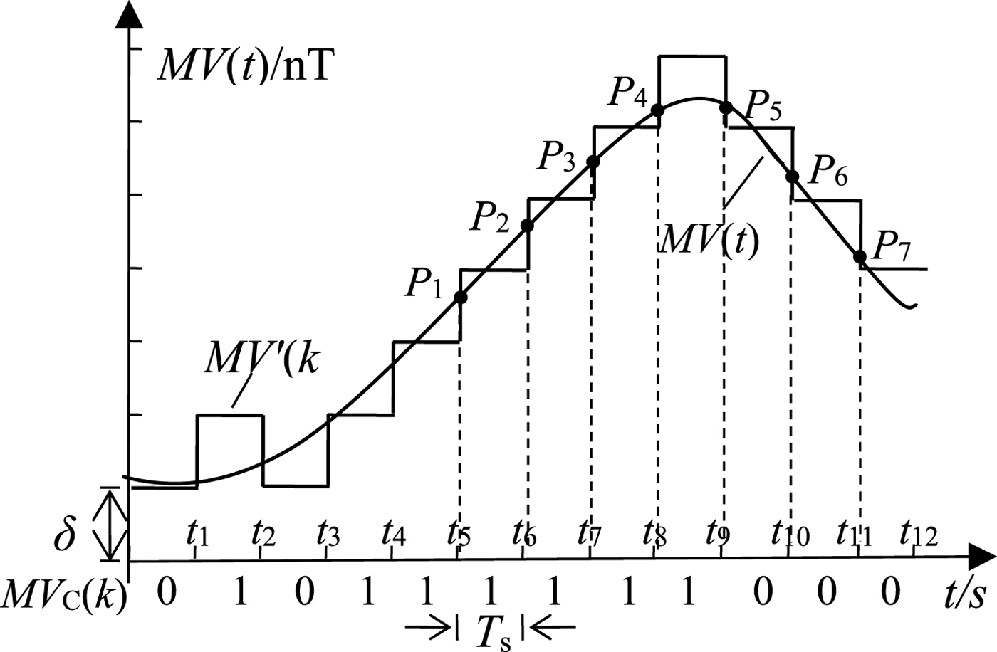
Figure 1. Schematic diagram of generating the GMS with the △M coding principle.
As is shown, MV(t) is encoded as “010111111000” according to the △M coding principle. When two codes “1” or “0” continuously appear in MVC (Equation (6) is met), the magnetic changes at the two sampling points are beyond the pre-set quantisation step δ. Then the INS's indicated position at the current sampling point is taken as an element of the matching sequence. For example, point P i (i = 1, 2, …, 7) in Figure 1 is one of the selected seven matching points. In this way, when the length of the GMS conforms, the △M-ICCP algorithm can be used for geomagnetic matching.
 $$MV_C (k) \oplus MV_C (k - 1) = 0, \quad k = 2, 3, \cdots, n - 1$$
where n is the length of MVC and “⊕” is the XOR operator.
An equal sampling interval is always applied in the traditional ICCP algorithm to generate the GMS. The algorithm based on △M coding is essentially a variable interval sampling method. In the magnetic field with obvious magnetic fluctuations, if the change of the magnetic field among adjacent matching points generated with an equal sampling interval is bigger than the quantisation step δ, the matching sequences obtained with the traditional ICCP and △M-ICCP algorithm are exactly the same. In this case, the former can be regarded as a special case of the latter. In the areas where the magnetic fluctuations are relatively flat, the sampling interval of the △M-ICCP algorithm is a multiple of the traditional ICCP algorithm.
3. PARAMETER DESIGN FOR △M-ICCP GEOMAGNETIC MATCHING ALGORITHM
3.1. Influences of matching length on the algorithm
Supposing m1 and m2 are two magnetic sequences which are sampled with an equal interval, denote △m as:
 $$\triangle{\bf m} = {\bf m}_{1} - {\bf m}_{2}$$
According to Nygren and Jansson's (Reference Nygren and Jansson2004) theory, if the absolute value of △m, namely, |△m|, varies within a very small range εm, then the two geomagnetic sequences are similar, and the probability of a false match will increase.
If m1 and m2 satisfy the Gaussian distribution, then the joint probability density function of △m can be expressed as:
 $$f(\Delta{\bf m}) = {1 \over \sqrt{(2\pi)^N \hbox{det}(C)}} e^{-{1 \over 2}\Delta{\bf m}C^{-1}\Delta{\bf m}}$$
where N is the length of the matching sequence and C is the covariance matrix of △m.
The simplest way to calculate the probability that the two sequences are close to each other is to de-correlate △m by a mode decomposition of C as:
 $$C = {\bf U \Lambda U}^T$$
where U is the eigenvector matrix and ᴧ is the eigenvalue matrix.
We substitute △m with Uy to compute an upper bound of the probability  $P(\vert \triangle{\bf m}\vert \le \varepsilon_{\rm m})$:
 $$P(\vert \Delta{\bf m}\vert \,{\le}\,\varepsilon_{\rm m})\,{\le}\,P(\vert \Delta{\bf m}\vert \,{\le}\,\varepsilon) = \int_{-\varepsilon}^\varepsilon\,{\cdots}\,\int_{-\varepsilon}^\varepsilon \Pi_{i=1}^N {e^{-{y_i^2 \over 2\lambda_i}} \over \sqrt{2\pi\lambda_i}} dy_1\,{\cdots}\,dy_N\,{=}\,\Pi_{i=1}^N \int_{-\varepsilon}^\varepsilon {e^{-{y_i^2 \over 2\lambda_i}} \over \sqrt{2\pi \lambda_i}} dy_i$$
where y = m1 + n, n is the measurement noise of the magnetic sensor and ε is a constant within εm. As the covariance matrix C is positive definite, so λi > 0, then:
 $$\int_{-\varepsilon}^\varepsilon {e^{-{y_i^2 \over 2\lambda_i}} \over \sqrt{2\pi \lambda_i}} dy_i < 1$$
It can be seen from Equations (10) and (11) that the probability of a false match decreases as the matching length increases. As the increase in matching length is equivalent to the increase in the matching distance in the equal interval sampling, to be more precise, the probability of a false match decreases as the matching distance increases. Since any non-Gaussian distribution can be approximated by a number of Gaussian functions, this conclusion still holds in the case that m1 and m2 follow the non-Gaussian distribution.
However, apart from the magnetic information, the matching distance is also influenced by other factors, such as sampling frequency, vehicle movement, and INS performance. Therefore, it is difficult to establish a precise model to calculate a reasonable matching distance. Although in the ICCP algorithm it is assumed that the magnetic sensor has no measurement error, in order to avoid confusion among magnetic measurements in practice, in the selection of δ, both the changes of magnetic field and the noise level after geomagnetic compensation should be considered.
According to the above analysis, the complicated step for establishing a model of matching length and the quantisation step are avoided. Instead, matching length and the quantisation step are jointly optimised to obtain the optimal solutions under certain conditions. In this way, the application requirements are met.
3.2. Parameter optimisation based on BPSO algorithm
The BPSO algorithm is a discrete intelligence optimisation algorithm with a simple principle and fast convergence. An estimation method of matching length L and quantisation step δ is proposed based on the BPSO algorithm as follows:
Step 1. Several calibration points are selected on a planning path to correct the INS's accumulated error and the set of calibration points is denoted as Pc.
Step 2. For one calibration point Pci, the search scope of δi and L i is set. According to the ΔM coding principle, when the magnetic fluctuation of the path is obvious, the quantisation step δ should be bigger; when they have less fluctuation, δ should be smaller. The variation analysis of the geomagnetic anomaly field model of NGDC-720 indicates that when the search scope of δ is between 1 nT and 15 nT, the practical requirements can be met. On the other hand, only when the matching length is greater than or equal to three (Besl and Mckay, Reference Besl and Mckay2002), can the ICCP algorithm can be operated. Therefore, the minimum value of the matching length is three. The maximum of L i is the length of the matching sequence generated with the maximal δi in its range on the trajectory before Pci. Both δi and L i are integers.
Step 3. δi and L i are encoded with binary code. Supposing  $\delta_{i} \in [1\,\hbox{nT}, 7\,\hbox{nT}]$ and L i∈[3, 30], then a three-digit numeric code is needed to encode δi and a five-digit numeric code for L i. Thus, the search range can be expressed as [00011001, 11110111], in which the first five codes represent L i and the last three codes represent δi.
Step 4. The swarms of the BPSO algorithm are randomly initialised and then the △M-ICCP algorithm is used to locate the vehicle with different δi and L i. For each combination of δi and L i, the “fitness” of each particle is calculated according to Equation (12) and the particle's position with the smallest fitness is stored in variable g best.
 $$f = \eta_1 f_1 (Er_{ij}) + \eta_2 f_2 (t_{ij})$$
where Eri,j is the matching error at point Pci with the matching parameters of swarm j, reflecting the matching accuracy, t ij is the average time required for one iteration in the algorithm, reflecting the time cost, f 1(Eri,j) and f 2(t ij) are respectively the normalised functions of Eri,j and t ij and η1 and η2 are adjustable factors for adjusting the weights of matching accuracy and time cost. The smaller the fitness, the better performance of the algorithm.
A linear mapping function f m(x) is defined. As shown in Figure 2, x can be normalised to the range [0, 1]; x 1 and x 2 are endpoints of the normalised interval and given based on the practical background.

Figure 2. Diagram of normalised functions.
Then f 1(Eri,j) and f 2(t ij), which respectively normalise Eri,j and t ij within [0, 1], can be expressed as:
 $$f_1 (Er_{ij}) = \left\{ \matrix{ \quad \; 0 \hfill &(Er_{ij} < Er_1) \cr {1 \over Er_2 - Er_1} (Er_{ij} - Er_1) &(Er_1 \le Er_{ij} < Er_2) \cr \quad \; 1 \hfill &(Er_{ij} \ge Er_2) } \right.$$
 $$f_2 (t_{ij}) = \left\{ \matrix{ \quad \; 0 \hfill &(t_{ij} < t_1) \cr {1 \over t_2 - t_1} (t_{ij} - t_1) &(t_1 \le t_{ij} < t_2) \cr \quad \; 1 \hfill &(t_{ij} \ge t_2) } \right.$$
where Er1, Er2, t 1, and t 2 are set according to the map's resolution and the accuracy and real-time performance required in the navigation system. In this paper, Er1 is the distance which is equal to a grid of the geomagnetic map, Er2 corresponds to the distance between two geomagnetic grids and t 1 and t 2 are respectively 0.5 s and 2 s.
Step 5. Velocities and positions of the swarms are updated with Equations (15) and (16). In the BPSO algorithm, the position X jd of swarm j only takes 0 or 1, but the velocity V jd, which represents the probability that X jd is 0 or 1, is not constrained.
 $$V_{jd} (k+1) = \omega V_{jd} (k) + c_1 r_1 (P_{jd} (k) - X_{jd} (k)) + c_2 r_2 (P_{gd} (k) - X_{jd} (k))$$
 $$X_{jd} (k+1) = \left\{ \matrix{ 1 &\rho_{jd} (k + 1) \le sigmoid(V_{jd} (k + 1)) \cr 0 &\rho_{jd} (k + 1) > sigmoid(V_{jd} (k + 1)) } \right.$$
where ω is the inertial weight, c 1 and c 2 are non-negative acceleration factors, r 1 and r 2 are random numbers within [0, 1], particle size j = 1, 2, … m, the dimension d = 1, 2, …, n and ρjd(k + 1) is a random value within (0, 1). The function sigmoid is defined as follows:
 $$sigmoid(x) = {1 \over 1 + \exp (-x)}$$
Step 6. All particles are evaluated according to their fitness. The fitness of the particles in the current iteration is compared with the individual optimum value p best and the global optimum value g best, and they are updated with new p best and g best with a smaller fitness.
Step 7. If the termination condition is met, stop the △M-ICCP algorithm and output g best. Otherwise, return to Step 5, update the particles’ velocities and positions and start the next iteration.
Step 8. Decode g best obtained in Step 7, and store the optimal matching length L i and quantisation step δi at Pci, which allows the smallest fitness in Equation (12).
The above method has the following three characteristics. First, the matching accuracy and time cost are directly used to construct the objective function in order to ensure the performance of the algorithm. Second, the efficiency of the algorithm is improved by generating a matching sequence with the geomagnetic information before the calibration point rather than accumulating a matching sequence from the calibration point. Third, the matching parameters of each calibration point can be calculated and stored offline in the path planning process and then directly called in the task execution phase. In this way, the algorithm's efficiency is further enhanced.
4. SIMULATION EXPERIMENTS
The geomagnetic anomaly field model NGDC-720 (Maus, Reference Maus2010) is applied to verify the proposed algorithm. First, two different local magnetic field areas are randomly selected from the model and the spans of their latitudes and longitudes are 2° (about 200 km). Then the Kriging interpolation method is used to establish the detailed magnetic maps, as shown in Figures 3 and 4. After interpolation, the resolution of the magnetic map is about 250 m. In Table 1, several statistical features of the two areas are provided. It is observed that the magnetic field in Area 1 changes more obviously than that in Area 2. Supposing that the vehicle is in the uniform rectilinear motion and its altitude does not change in the geomagnetic matching process, several paths are randomly generated in each area to verify the △M-ICCP algorithm. The magnetic changes in three different paths are shown in Figures 3 and 4. The marker “○” indicates the starting point and “*” indicates the selected calibration point.
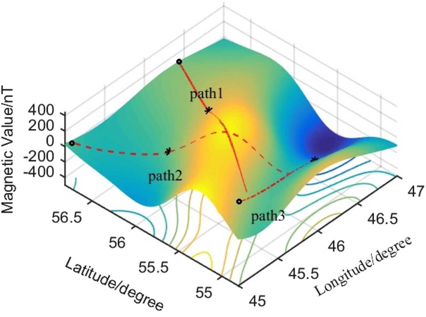
Figure 3. Magnetic field in Area 1.
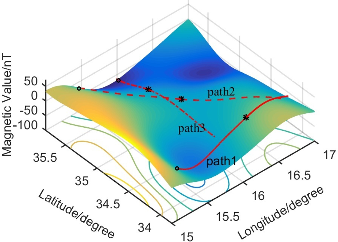
Figure 4. Magnetic field in Area 2.
Table 1. Statistical features of the two magnetic areas.

Taking Path 1 in Areas 1 and 2 as examples, first, the method in Section 3.2 is used to evaluate the optimal matching length L and quantisation step δ offline at the calibration point of each path. As the magnetic field in Area 1 varies significantly, the search ranges of L and δ can be expanded appropriately to ensure the matching accuracy. In Area 2, since the magnetic fluctuation is small, the search ranges can be narrowed to avoid a long matching distance. Therefore, the search ranges of δ and L of Path 1 in Area 1 are set in the ranges of [1 nT, 15 nT] and [3, 31]. Similarly, δ and L of Path 1 in Area 2 are searched in the ranges of [1 nT, 8 nT] and [3, 10]. The swarm's population in the BPSO algorithm is 30, and the iterative time is 100. Fitness of Path 1 in Areas 1 and 2 are shown in Figures 5 and 6.

Figure 5. Fitness under different δ and L in Area 1.

Figure 6. Fitness under different δ and L in Area 2.
As the matching precision and time cost differ when δ and L vary, the corresponding fitness is different. It is observed that although time consumption of the algorithm is less under the smaller δ and L, the matching precision cannot be guaranteed and the fitness is bigger. When δ and L are increased to a certain extent, the fitness is the smallest. In this case, the time cost is reduced and the accuracy is guaranteed. For Path 1 in Area 1, when δ = 15 and L = 22, where the flag is located, the fitness achieves a minimum value of 1.41. This means that the better matching results can be obtained when the optimised parameters are used to generate the GMS. For Path 1 in Area 2, when δ = 7 and L = 7, the fitness is the smallest and reaches 0.
The performances of the adaptive △M-ICCP and the traditional ICCP algorithm are experimentally compared. The experiments are described as follows. Firstly, the GMS of the traditional ICCP algorithm is generated with equal sampling interval and the matching length is the same as with the △M-ICCP algorithm. Secondly, the GMS of the traditional ICCP algorithm is sampled with an equal interval and the matching distance is equal to the △M-ICCP algorithm. To improve the efficiency, according to the statistical characteristics of the INS's errors, the search areas of the △M-ICCP and ICCP algorithm are both set within ±3σ, where σ is the INS's drift generated since the former update.
Path 1 in Area 1 and Area 2 are selected for analysis. It is assumed that the vehicle is in uniform rectilinear motion at the speed of 35 m/s. As the effects of different error sources on the ICCP algorithm can be attributed to the effects of position error, the position error is considered in the experiments. When the vehicle arrives at the calibration point, we suppose the accumulated error is 790 m. The experiments were performed according to the comparative schemes above and L and δ of the △M-ICCP algorithm were designed using the BPSO algorithm. The equal sampling interval of the traditional ICCP algorithm is 24 s, which satisfies Equations (1) and (2). The matching error of the algorithm is calculated according to Equation (18):
 $$E_{RMSE} = \sqrt{{1 \over L} \sum\limits_{i=1}^L (MP_i - P_i)^2}$$
where L is the matching length, MP is the matching result and P is the ideal position.
In the geomagnetic matching process, the number of iterations is 300. When the matching error between two adjacent iterations is less than 1 m, the matching algorithm terminates. Figures 7 and 8 show the matching errors and the magnetic values of each matching point in Areas 1 and 2.

Figure 7. Matching results of Path 1 in Area 1. (a) Matching errors of different algorithms.(b) Magnetic values of different matching sequences.

Figure 8. Matching results of Path 1 in Area 2. (a) Matching errors of different algorithms. (b) Magnetic values of different matching sequences.
In Figure 7(a), all matching algorithms can reduce the INS's accumulated error. However, when the matching length is the same, the matching error of the ICCP algorithm is 665.30 m, which is more than two grids in the magnetic map; the matching error of the △M-ICCP algorithm is 267.97 m. As shown in Figure 7(b), when the matching lengths of the two algorithms are the same, the △M-ICCP algorithm can utilise more magnetic information, thus ensuring the algorithm's matching accuracy. When matching distances are the same, since the △M-ICCP algorithm controls the magnetic changes of the GMS, fewer points are used in the matching process. Therefore, the algorithm's efficiency is improved.
Similarly, in Figure 8(a), when the matching lengths are the same, the matching error of the traditional ICCP algorithm is 784.53 m, which cannot be used to correct the INS's accumulated error. As mentioned above, the overall magnetic fluctuation in Area 2 is less obvious. When the sampling interval is too small, magnetic values of the matching points are very close, thus the available magnetic information is limited. To improve the accuracy of the algorithm, the matching distance needs to be increased to enrich the magnetic information. In Figure 8(a), the traditional ICCP and M-ICCP algorithm with a longer matching distance achieves the better matching results. Their matching errors are respectively 161.65 m and 159.92 m.
To sum up, the proposed adaptive △M-ICCP algorithm can select the optimal parameters according to different paths and magnetic areas, thus providing a guideline for generating the GMS.
To fully verify the algorithm, more paths are randomly generated in Areas 1 and 2 for geomagnetic matching. It is assumed that the simulation conditions and the INS's accumulated error do not change. Tables 2 and 3 show the matching results of the selected paths.
Table 2. Comparison of different algorithms with the same matching length.

Table 3. Comparison of different algorithms with the same matching distance.
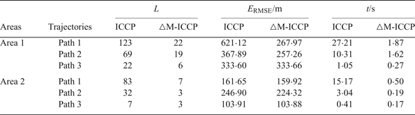
In Table 2, the matching sequences of the traditional ICCP algorithm and ΔM-ICCP algorithm have the same length, but their matching distances are different. It is obvious that the matching errors in all paths of the △M-ICCP algorithm are smaller than those of the traditional ICCP algorithm. Furthermore, matching results of the △M-ICCP on Path 1 and Path 2 in Area 1 and Path 1 in Area 2 are much better than those of the traditional ICCP algorithm. It can also be observed that the time consumption of the two algorithms is similar when their matching lengths are the same. Comparing the traditional ICCP algorithms in Tables 2 and 3, the matching lengths in Table 3 are longer and corresponding matching results are improved, but the matching time increases.
In Table 3, the matching distances of the traditional ICCP algorithm and the △M-ICCP algorithm are the same, but the matching lengths are different. Clearly, the matching performances of △M-ICCP algorithm are better than the traditional one, and the time consumption of the former is much shorter than the latter. On Path 1 in Area 1 and Path 1 and Path 2 in Area 2, the time consumption decreases significantly. Experiments also indicate that the △M-ICCP algorithm can generally achieve the best results and the matching sequence is not too long.
Based on all the results in Figures 7 and 8 and Tables 2 and 3, the following conclusions can be drawn. First, matching length mainly affects the search time of the ICCP algorithm. With the same matching length, the time cost of the traditional ICCP algorithm is equivalent to that of the △M-ICCP algorithm. The longer the sequence, the greater the time cost. Second, the matching distance mainly influences the algorithm's accuracy. To some extent, increasing matching distance can enrich the information of the matching sequence and improve the matching accuracy. Third, the proposed △M-ICCP algorithm can adaptively adjust the parameters to generate the GMS according to the magnetic information, thus guaranteeing the matching accuracy and reducing the time consumption to the greatest extent. It should be noted that since the most accurate matching algorithm can only limit the matching accuracy within one grid of the reference map, the precision of the algorithm can be further improved by increasing the resolution of geomagnetic maps.
5. CONCLUSIONS
An adaptive △M-ICCP geomagnetic matching algorithm is presented based on the △M coding principle, which is used to generate the GMS for geomagnetic navigation. By selecting suitable objective functions, the problem of designing matching length and quantisation step for the △M-ICCP algorithm is turned into an optimisation problem. The proposed algorithm can adjust its parameters according to the magnetic information on the path and the requirements of the navigation system in diverse application backgrounds. Simulation experiments proved the validity of the algorithm. Even in a magnetic field with less obvious fluctuations, the algorithm can also obtain valid matching results. With the continuous improvements in geomagnetic modelling and mapping, the accuracy of the △M-ICCP algorithm will be further improved. In addition, the proposed algorithm can also be combined with other modified strategies such as constructing a slide window to limit its search scope to further increase the performance of the algorithm.


