


1. Introduction
Viscoelastic flows have been of interest ever since the observation 70 years ago that a substantial reduction in viscous drag on a wall of a pipe carrying turbulent flow is possible after adding only a few parts per millon of long-chain polymers (Toms Reference Toms1948) – just as, curiously, adding further polymer quickly saturates this effect when the so-called ‘maximum drag reduction’ (MDR) regime is entered (Virk Reference Virk1970), with skin friction reduced by  $\sim$80% relative to its Newtonian value. Efforts to explain this phenomenon have naturally focused on understanding how low polymer concentrations moderate Newtonian turbulence (e.g. Lumley Reference Lumley1969; Tabor & de Gennes Reference Tabor and de Gennes1986; Procaccia, Lvov & Benzi Reference Procaccia, Lvov and Benzi2008; White & Mungal Reference White and Mungal2008). However, the discovery of a new form of viscoelastic turbulence – ‘elasto-inertial’ turbulence (EIT) – in 2013 (Dubief, Terrapon & Soria Reference Dubief, Terrapon and Soria2013; Samanta et al. Reference Samanta, Dubief, Holzner, Schäfer, Morozov, Wagner and Hof2013; Sid, Terrapon & Dubief Reference Sid, Terrapon and Dubief2018), which exists at large Reynolds number
  $Re = O(10^3)$ and Weissenberg number
  $Wi=O(10)$, has provided a competing and even less well understood possibility. Provided that
  $Wi$ is large enough, EIT can exist at much lower
  $Re$ than Newtonian turbulence, explaining what has been labelled in the past as ‘early turbulence’ (Jones & Maddock Reference Jones and Maddock1966; Goldstein, Adrian & Kreid Reference Goldstein, Adrian and Kreid1969; Hansen & Little Reference Hansen and Little1974; Draad, Kuiken & Nieuwstadt Reference Draad, Kuiken and Nieuwstadt1998; Samanta et al. Reference Samanta, Dubief, Holzner, Schäfer, Morozov, Wagner and Hof2013; Chandra, Shankar & Das Reference Chandra, Shankar and Das2018; Choueiri, Lopez & Hof Reference Choueiri, Lopez and Hof2018). At higher but fixed
  $Re$, it is also possible, as the polymer concentration is steadily increased from zero, to relaminarize Newtonian turbulence before triggering EIT (Choueiri et al. Reference Choueiri, Lopez and Hof2018; Chandra et al. Reference Chandra, Shankar and Das2018). In direct numerical simulations (DNS), increasing
  $Wi$ from a state of EIT quenches the flow down to a simple travelling wave solution and presumably laminar flow if
  $Wi$ is large enough (e.g. see figure 2 in Page, Dubief & Kerswell Reference Page, Dubief and Kerswell2020; Dubief et al. Reference Dubief, Page, Kerswell, Terrapon and Steinberg2020). At even higher
  $Re$, it is currently unclear whether the two types of turbulence merge or co-exist, and how MDR fits into the situation remains an outstanding issue (e.g. Xi & Graham Reference Xi and Graham2010, Reference Xi and Graham2012; Samanta et al. Reference Samanta, Dubief, Holzner, Schäfer, Morozov, Wagner and Hof2013; Graham Reference Graham2014; Choueiri et al. Reference Choueiri, Lopez and Hof2018, Reference Choueiri, Lopez, Varshey, Sankar and Hof2021; Lopez, Choueiri & Hof Reference Lopez, Choueiri and Hof2019).
Further questions also exist as to how EIT relates to another form of viscoelastic turbulence – ‘elastic’ turbulence (ET) – that was discovered a decade earlier (Groisman & Steinberg Reference Groisman and Steinberg2000). This is generated by the well-known ‘elastic’ linear instability of curved streamlines (Larson, Shaqfeh & Muller Reference Larson, Shaqfeh and Muller1990; Shaqfeh Reference Shaqfeh1996) and exists at vanishingly small Reynolds numbers so inertial effects are unambiguously irrelevant for sustaining the turbulence. This elastic instability is also possible in planar geometries, but requires finite-amplitude disturbances to generate streamline curvature (Meulenbroek et al. Reference Meulenbroek, Storm, Morozov and van Saarloos2004; Morozov & Saarloos Reference Morozov and Saarloos2007). Intriguingly, substantial linear transient growth can occur in the purely elastic limit via a polymeric ‘lift-up’ effect, with streaks in the streamwise velocity (Jovanović & Kumar Reference Jovanović and Kumar2010, Reference Jovanović and Kumar2011), but is very different in appearance to these finite-amplitude solutions. In contrast to the inertialess ET, a fairly large  $Re$ is required for EIT, indicating that inertia is important here. This suggests that EIT and ET are distinct phenomena (e.g. see figure 30 of Chaudhary et al. Reference Chaudhary, Garg, Subramanian and Shankar2021) yet they could still be two extremes of the same whole (Samanta et al. Reference Samanta, Dubief, Holzner, Schäfer, Morozov, Wagner and Hof2013; Qin et al. Reference Qin, Salipante, Hudson and Arratia2019; Choueiri et al. Reference Choueiri, Lopez, Varshey, Sankar and Hof2021; Steinberg Reference Steinberg2021). Finally, the underlying mechanism that sustains EIT has yet to be clarified (Dubief et al. Reference Dubief, Terrapon and Soria2013; Terrapon, Dubief & Soria Reference Terrapon, Dubief and Soria2015; Sid et al. Reference Sid, Terrapon and Dubief2018; Shekar et al. Reference Shekar, MucMullen, Wang, McKeon and Graham2018, Reference Shekar, MucMullen, McKeon and Graham2020; Page et al. Reference Page, Dubief and Kerswell2020; Chaudhary et al. Reference Chaudhary, Garg, Subramanian and Shankar2021).
A major step forward in explaining the origin of EIT was made recently when a linear instability was found at relatively high  $Wi \gtrsim 20$, which could reach down to a threshold
  $Re_c \approx 63$ in pipe flow (Garg et al. Reference Garg, Chaudhary, Khalid, Shankar and Subramanian2018; Chaudhary et al. Reference Chaudhary, Garg, Subramanian and Shankar2021). This finding overturned a long-held view that no new linear instability would appear by adding polymers to a Newtonian rectilinear shear flow: see Chaudhary et al. (Reference Chaudhary, Garg, Shankar and Subramanian2019, Reference Chaudhary, Garg, Subramanian and Shankar2021) for an extensive historical discussion of this point, and the recent review by Sanchez et al. (Reference Sanchez, Jovanovic, Kumar, Morozov, Shankar, Subramanian and Wilson2022). This instability was also confirmed in channel flow (Khalid et al. Reference Khalid, Chaudhary, Garg, Shankar and Subramanian2021a) using an Oldroyd-B fluid, but was found absent in an upper-convected Maxwell fluid (Chaudhary et al. Reference Chaudhary, Garg, Shankar and Subramanian2019). The instability is a centre-mode instability that has a phase speed close to the maximum base flow speed and appeared to need inertia (finite
  $Re$) to exist – in a channel with an experimentally relevant
  $\beta$ (the ratio of solvent-to-solution viscosities) of
  $0.9$ and elasticity number
  $0.1$, the threshold
  $Re_c \approx 200$ (Khalid et al. Reference Khalid, Chaudhary, Garg, Shankar and Subramanian2021a) consistent with the finite threshold of
  $Re_c \approx 63$ found earlier in pipe flow (Garg et al. Reference Garg, Chaudhary, Khalid, Shankar and Subramanian2018; Chaudhary et al. Reference Chaudhary, Garg, Subramanian and Shankar2021). However, in the dilute limit (
 $\beta \rightarrow 1$) and in contrast with pipe flow, Khalid et al. (Reference Khalid, Chaudhary, Garg, Shankar and Subramanian2021a) also found that
  $Re_c$ could be pushed down to approximately
  $5$ by the time
  $\beta$ reached
  $0.99$, albeit at very large
  $Wi$ (
 $=O(10^3)$). Further computations (Khalid, Shankar & Subramanian Reference Khalid, Shankar and Subramanian2021b) have confirmed that the elastic limit of
  $Re=0$ can indeed be reached at
  $\beta =0.9905$ and
  $Wi\approx 2500$. Looking beyond the extreme value of
  $Wi$ – which is apparently achievable experimentally (Vashney & Steinberg Reference Vashney and Steinberg2018; Schnapp & Steinberg Reference Schnapp and Steinberg2021) – this result has established a fascinating connection between an instability that appears to need inertia, elasticity and solvent viscosity (finite
  $(1-\beta )$) and a purely elastic instability when
  $(1-\beta )$ is small enough (Khalid et al. (Reference Khalid, Shankar and Subramanian2021b) refer to this as an ‘ultra dilute’ polymer solution).
However, EIT appears at lower  $Wi$ (figure 2 in Page et al. Reference Page, Dubief and Kerswell2020) and sometimes lower
  $Re$ at a given
  $Wi$ (see figure 1(b) in Choueiri et al. Reference Choueiri, Lopez, Varshey, Sankar and Hof2021) than the centre-mode instability. For example, in channel flow at
  $Re=1000$ and
  $\beta =0.9$ in an FENE-P fluid with
  $L_{max}=500$, EIT occurs around
  $Wi=20$, whereas the centre-mode instability threshold is
  $Wi \approx 70$ (figure 2 (left) in Page et al. Reference Page, Dubief and Kerswell2020). This means that if EIT is connected dynamically to this instability, then the hierarchy of nonlinear solutions that emerge from the linear instability must be substantially subcritical, reaching to
  $Wi$ values far below those of the neutral curve (and similarly for
  $Re$ for high enough
  $Wi$). This was confirmed in one specific case on the neutral curve –
  $(Re,Wi,\beta )=(60,26.9,0.9)$ – where the bifurcation was shown to be strongly subcritical, with the branch of travelling wave solutions reaching down to
  $Wi=8.77$ (Page et al. Reference Page, Dubief and Kerswell2020). Moreover, the travelling wave solutions adopt a distinctive ‘arrowhead’ form in the polymer stress when
  $Wi$ is small enough, which can be recognized as an intermittently observed coherent structure in the DNS of EIT (Dubief et al. Reference Dubief, Page, Kerswell, Terrapon and Steinberg2020).
The primary purpose of this paper is to back up this initial finding of subcriticality by carrying out a systematic survey of whether the centre-mode bifurcation is subcritical or supercritical across the entire neutral curve for a typical value of  $\beta$ of
  $0.9$ using weakly nonlinear analysis (Stuart Reference Stuart1960; Watson Reference Watson1960). In doing so, we also take the opportunity to confirm that the instability is present for an FENE-P fluid with reasonable maximum polymer extension
  $L_{max}$ (see (2.1d)) and, spurred on by the recent results of Khalid et al. (Reference Khalid, Shankar and Subramanian2021b), explore how the presence of finite
  $L_{max}$ affects the dilute limit (
 $\beta \rightarrow 1$) where
  $Re=0$ can be reached. We also examine the energetic source term, or terms, for the instability, uncovering a consistent picture even on the part of the neutral curve reaching to high
  $Re$.
$Re$.
The plan of the paper is as follows. In § 2, the FENE-P model is introduced and the presence or not of polymer diffusion as indicated by a Schmidt number  $Sc$ is discussed. The weakly nonlinear expansions are also introduced. While this is now an established method in the fluid dynamicists’ toolbox, for viscoelastic models where the (coarse-grained) local polymer configuration is represented by a positive definite conformation tensor
  $\boldsymbol{\mathsf{C}}$, there are some technicalities that need some attention. We follow the framework suggested recently by Hameduddin et al. (Reference Hameduddin, Meneveau, Zaki and Gayme2018) and Hameduddin, Gayme & Zaki (Reference Hameduddin, Gayme and Zaki2019) to treat this issue, which requires a bit more formal development than is normal. Having set this up, § 3 then presents the weakly nonlinear analysis, which proceeds as usual albeit with a proxy for
  $\boldsymbol{\mathsf{C}}$ being expanded instead of
  $\boldsymbol{\mathsf{C}}$ itself. Results in § 4 are arranged as follows: §§ 4.1 and 4.2 consider
  $(\beta,L_{max})=(0.9,500)$ with
  $Sc\to \infty$; § 4.3 considers
  $(\beta,L_{max},Sc)=(0.9,100,10^6)$; § 4.4 performs an energy analysis over the neutral curves of §§ 4.1 and 4.3; and finally § 4.5 examines the
  $Re=0$ situation, varying
  $\beta$ over the approximate range
  $[0.97,0.99]$ for
  $Wi \leqslant 200$ and
  $L_{max} \in [40,100]$ (
 $Sc\to \infty$). More moderate
  $\beta$ are considered in Appendix C, specifically
  $(\beta, L_{max})=(0.74, \{250,500,\infty \})$ and
  $(0.56,\{ 500, \infty \})$ (all at
  $Sc \to \infty$). Lastly, § 5 presents a discussion of the paper's results.
While this work was going through review, we became aware of the complementary work of Wan, Sun & Zhang (Reference Wan, Sun and Zhang2021) on the weakly nonlinear analysis of axisymmetric pipe flow. Their findings are consistent with those reported here for channel flow.
2. Formulation
We consider pressure-driven viscoelastic flow between two parallel stationary rigid plates separated by a distance  $2h$ and assume that the flow is governed by the FENE-P model
 $$\begin{gather} \partial_t \boldsymbol{u} + \left( \boldsymbol{u} \boldsymbol{\cdot} \boldsymbol{\nabla} \right) \boldsymbol{u} + \boldsymbol{\nabla} p = \frac{\beta}{Re}\,\Delta \boldsymbol{u} + \frac{1-\beta}{Re}\,\boldsymbol{\nabla} \boldsymbol{\cdot} \boldsymbol{\mathsf{T}}(\boldsymbol{\mathsf{C}}), \end{gather}$$
 $$\begin{gather}\boldsymbol{\nabla} \boldsymbol{\cdot} \boldsymbol{u} =0, \end{gather}$$
 $$\begin{gather}\partial_t \boldsymbol{\mathsf{C}} + \left( \boldsymbol{u} \boldsymbol{\cdot} \boldsymbol{\nabla}\right) \boldsymbol{\mathsf{C}} + \boldsymbol{\mathsf{T}}(\boldsymbol{\mathsf{C}}) = \boldsymbol{\mathsf{C}} \boldsymbol{\cdot} \boldsymbol{\nabla} \boldsymbol{u} + \left( \boldsymbol{\nabla} \boldsymbol{u} \right)^{T} \boldsymbol{\cdot} \boldsymbol{\mathsf{C}} + \frac{1}{Re\,Sc}\,\Delta \boldsymbol{\mathsf{C}}. \end{gather}$$
The constitutive relation for the polymer stress,  $\boldsymbol{\mathsf{T}}$, is given by the Peterlin function
 \begin{equation} \boldsymbol{\mathsf{T}}(\boldsymbol{\mathsf{C}}) := \frac{1}{Wi} \left(\, f (\mathrm{tr} \, \boldsymbol{\mathsf{C}})\,\boldsymbol{\mathsf{C}} - {\boldsymbol{\mathsf{I}}} \right), \quad {\rm where} \ f(x) := \left(1-\frac{x-3}{L^2_{max}}\right)^{{-}1}, \end{equation}
with  $L_{max}$ denoting the maximum extensibility of polymer chains. Here,
  $\boldsymbol{\mathsf{C}} \in \mathrm {Pos}(3)$ (the set of positive definite
  $3 \times 3$ matrices) is the polymer conformation tensor, and
  $\beta \in [0,1]$ denotes the viscosity ratio
  $\beta := \nu _s/\nu$, where
  $\nu _s$ and
  $\nu _p=\nu -\nu _s$ are the solvent and polymer contributions to the total kinematic viscosity
  $\nu$. The equations are non-dimensionalized by
  $h$ and the bulk speed
 \begin{equation} U_b:= \frac{1}{2h} \int^h_{{-}h} u_x\, {{\rm d} y} \end{equation}
which, through adjusting the pressure gradient appropriately, is kept constant so that the Reynolds and Weissenberg numbers are defined as
 \begin{equation} Re:= \frac{hU_b}{\nu}, \quad Wi:= \frac{\tau U_b}{h}, \end{equation}
where  $\tau$ is the polymer relaxation time. Polymer diffusion – the last term in (2.1c) – is often omitted as the typical magnitude of the Schmidt number,
  $Sc \sim O( 10^6)$. Here it is retained throughout the nonlinear analysis to: (i) allow a more realistic comparison with results from DNS, where a relatively low Schmidt number (
 $Sc \sim O( 10^3)$) is required for the solver to converge (Page et al. Reference Page, Dubief and Kerswell2020); and (ii) assess its importance more generally. Non-slip boundary conditions are imposed on the velocity field. If an infinite Schmidt number
  $Sc$ is considered, then no boundary conditions for the conformation tensor
  $\boldsymbol{\mathsf{C}}$ are needed. In the case of finite Schmidt numbers, we apply
  $Sc\to \infty$ at the boundary to retain this situation (Sid et al. Reference Sid, Terrapon and Dubief2018).
In the course of this work, we compute neutral curves for the recently discovered centre-mode instability (Garg et al. Reference Garg, Chaudhary, Khalid, Shankar and Subramanian2018) in a channel following the recent work by Khalid et al. (Reference Khalid, Chaudhary, Garg, Shankar and Subramanian2021a,Reference Khalid, Shankar and Subramanianb). The marginally-stable eigenfunctions form the basis of a weakly nonlinear expansion in the amplitude of the bifurcating solution. The key objective here is to ascertain whether the bifurcation is supercritical or subcritical. Subcriticality would indicate that bifurcated solutions exist beyond the parameter domain of linear instability, thereby implying that the flow is nonlinearly unstable – i.e. unstable to sufficiently large amplitude disturbances – in new, potentially more interesting parameter regimes. A case in point is the very recent discovery that the centre-mode instability still operates at  $Re=0$, albeit at very high
  $Wi=O(1000)$ and ultra-dilute polymer solutions of
  $1-\beta =O(10^{-3})$ (Khalid et al. Reference Khalid, Shankar and Subramanian2021b). While these extremes are on the margins of physical relevance, a strongly subcritical instability could still see its consequences in the form of finite-amplitude solutions at vastly different
  $Wi$ and
  $\beta$.
2.1. Base state
The base state to (2.1a)–(2.1c) is the steady unidirectional solution and satisfies the following reduced set of equations:
 $$\begin{gather} \partial_x p = \frac{\beta}{Re}\,\partial_{yy} u_x + \frac{1-\beta}{Re\,Wi} \left[ \frac{\left(f (\mathrm{tr} \, \boldsymbol{\mathsf{C}}) \right)^2}{L^2_{max}}\,\mathrm{tr} (\partial_y \boldsymbol{\mathsf{C}})\,{\mathsf{C}}_{xy}+f (\mathrm{tr} \, \boldsymbol{\mathsf{C}})\,\partial_y {\mathsf{C}}_{xy}\right], \end{gather}$$
 $$\begin{gather}\frac{1}{Wi} \left(\, f (\mathrm{tr} \, \boldsymbol{\mathsf{C}})\,{\mathsf{C}}_{xx}-1 \right) = 2{\mathsf{C}}_{xy}\,\partial_y u_x + \frac{1}{Re\,Sc}\,\partial_{yy} {\mathsf{C}}_{xx}, \end{gather}$$
 $$\begin{gather}\frac{1}{Wi} \left(\, f (\mathrm{tr} \, \boldsymbol{\mathsf{C}})\,{\mathsf{C}}_{yy}-1 \right) = \frac{1}{Re\,Sc}\,\partial_{yy} {\mathsf{C}}_{yy}, \end{gather}$$
 $$\begin{gather}\frac{1}{Wi} \left(\, f (\mathrm{tr} \, \boldsymbol{\mathsf{C}})\,{\mathsf{C}}_{zz}-1 \right) = \frac{1}{Re\,Sc}\,\partial_{yy} {\mathsf{C}}_{zz}, \end{gather}$$
 $$\begin{gather}\frac{1}{Wi} \left(\, f (\mathrm{tr} \, \boldsymbol{\mathsf{C}})\,{\mathsf{C}}_{xy} \right) = {\mathsf{C}}_{yy} \partial_y u_x + \frac{1}{Re\,Sc}\,\partial_{yy} {\mathsf{C}}_{xy}, \end{gather}$$
where  $\boldsymbol {u}=u_x \hat {\boldsymbol {x}}+u_y \hat {\boldsymbol {y}}$. Since
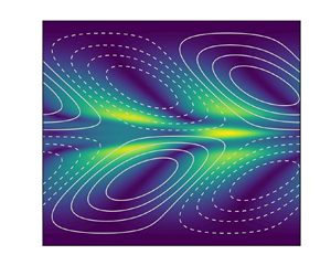
  $Re$ is based on the bulk speed, the applied pressure gradient is adjusted until the bulk speed is unity (after non-dimensionalization) (e.g. Dubief et al. Reference Dubief, Terrapon and Soria2013, Reference Dubief, Page, Kerswell, Terrapon and Steinberg2020; Samanta et al. Reference Samanta, Dubief, Holzner, Schäfer, Morozov, Wagner and Hof2013; Sid et al. Reference Sid, Terrapon and Dubief2018). Figure 1 displays the base state
  $(\boldsymbol {u}_b,p_b,\boldsymbol{\mathsf{C}}_b)$ for a particular parameter combination. It is worth remarking that
  $U_{max}$ is very nearly
  $1.5$ in units of
  $U_b$ for
  $\beta$ close to 1 (e.g.
  $\beta =0.9$, which is used in the main part of the paper) and then
  $Wi$ based on the bulk velocity (as here) is very close to two-thirds of a Weissenberg number based on
  $U_{max}$ (Garg et al. Reference Garg, Chaudhary, Khalid, Shankar and Subramanian2018; Chaudhary et al. Reference Chaudhary, Garg, Subramanian and Shankar2021; Khalid et al. Reference Khalid, Chaudhary, Garg, Shankar and Subramanian2021a,Reference Khalid, Shankar and Subramanianb). In Appendix C, we consider
  $\beta =0.56$ and
  $\beta =0.74$, where this simple relationship no longer holds.

Figure 1. Laminar base state at  $\beta =0.9$,
  $L_{max} =500$,
  $Sc \to \infty$,
  $Wi = 60$,
  $Re = 68$. The components of the base flow conformation tensor,
  $\boldsymbol{\mathsf{C}}_b$, are normalized by their values at the bottom wall (
 $y = -1$):
  ${\mathsf{C}}_{b,xx} \vert _{y=-1}=39\,235$,
  ${\mathsf{C}}_{b,yy} \vert _{y=-1}={\mathsf{C}}_{b,zz} \vert _{y=-1}=0.84$,
  ${\mathsf{C}}_{b,xy} \vert _{y=-1} = 129$.
2.2. Perturbative expansions
The weakly nonlinear expansions for the velocity and pressure components are written straightforwardly in the form
 \begin{equation} \boldsymbol{u} = \boldsymbol{u}_{b} + \sum_{k=1}^{N} \varepsilon^k \boldsymbol{u}_{(k)}, \quad p = p_{b} + \sum_{k=1}^{N} \varepsilon^k p_{(k)}. \end{equation}
However, the conformation tensor  $\boldsymbol{\mathsf{C}}$ calls for a more careful treatment, since the set of positive definite
  $3 \times 3$ matrices,
  $\mathrm {Pos} (3)$, cannot be a vector space. Instead, it may be endowed with the structure of a complete Riemannian manifold. Perturbations of order
  $\varepsilon ^k$ still make sense in this setting, but one has to interpret the
  $\varepsilon ^k$ distance in terms of the metric arising from the Riemannian structure of the manifold
  $\mathrm {Pos} (3)$. In developing perturbations for the conformation tensor
  $\boldsymbol{\mathsf{C}}$, we follow the framework of Hameduddin et al. (Reference Hameduddin, Meneveau, Zaki and Gayme2018, Reference Hameduddin, Gayme and Zaki2019), who focused on precisely this issue. We may view
  $\boldsymbol{\mathsf{C}}$ as the left Cauchy–Green tensor associated with the polymer deformation, i.e.
 \begin{equation} \boldsymbol{\mathsf{C}} = \boldsymbol{\mathsf{F}} {\boldsymbol{\mathsf{F}}}^{T}, \end{equation}
where  $\boldsymbol{\mathsf{F}}$ denotes the deformation gradient with thermal equilibrium taken as the reference configuration. A further decomposition of
  $\boldsymbol{\mathsf{F}}$ into two successive deformations, which may be written as
 \begin{equation} \boldsymbol{\mathsf{F}} = \boldsymbol{\mathsf{F}}_{b} \boldsymbol{\mathsf{L}}, \end{equation}
separates the deformation corresponding to the perturbation,  $\boldsymbol{\mathsf{L}}$, from the deformation associated with the base state, which may be expressed as
 \begin{equation} \boldsymbol{\mathsf{F}}_{b} = \boldsymbol{\mathsf{C}}_{b}^{{1}/{2}}. \end{equation}
(This representation is not unique; any  $\boldsymbol{\mathsf{F}}_{b} = \boldsymbol{\mathsf{C}}_{b}^{{1}/{2}} {\boldsymbol{\mathsf{R}}}$ works with
  ${\boldsymbol{\mathsf{R}}} \in \mathrm {SO}(3)$. The choice
  ${\boldsymbol{\mathsf{R}}}={\boldsymbol{\mathsf{I}}}$ is natural in the sense that it allows for a geodesic between
  $\boldsymbol{\mathsf{C}}_{b}$ and
  $\boldsymbol{\mathsf{C}}$ to be expressed solely in terms of
  $\boldsymbol{\mathsf{F}}_{b}$ and
  $\boldsymbol{\mathsf{G}}$.)
The fluctuating deformation gradient  $\boldsymbol{\mathsf{L}}$ has an associated left Cauchy–Green tensor
  $\boldsymbol{\mathsf{G}}=\boldsymbol{\mathsf{L}} {\boldsymbol{\mathsf{L}}}^{T}$. Combining these observations, we have that
 \begin{equation} \boldsymbol{\mathsf{C}} = \boldsymbol{\mathsf{F}}_{b} \boldsymbol{\mathsf{G}} {\boldsymbol{\mathsf{F}}}_{b}^{T}. \end{equation}
The tensor  $\boldsymbol{\mathsf{G}}$ is necessarily positive definite since
  $\boldsymbol{\mathsf{C}}$ is, and by nature it acts as the conformation tensor representing the fluctuations of
  $\boldsymbol{\mathsf{C}}$ around
  $\boldsymbol{\mathsf{C}}_{b}$.
The evolution equation (2.1c) for the conformation tensor can be rewritten in terms of  $\boldsymbol{\mathsf{G}}$ as
 \begin{equation} \partial_t \boldsymbol{\mathsf{G}} + (\boldsymbol{u} \boldsymbol{\cdot} \boldsymbol{\nabla}) \boldsymbol{\mathsf{G}} = 2\,\mathrm{sym} \left(\boldsymbol{\mathsf{G}}\,h(\boldsymbol{u}) \right) - {\boldsymbol{\mathsf{F}}}_{b}^{{-}1} \boldsymbol{\mathsf{T}} {\boldsymbol{\mathsf{F}}}_{b}^{{-}T}, \end{equation}
with
 \begin{equation} h (\boldsymbol{u}) = {\boldsymbol{\mathsf{F}}}_{b}^{T} \boldsymbol{\cdot} \boldsymbol{\nabla} \boldsymbol{u} \boldsymbol{\cdot} {\boldsymbol{\mathsf{F}}}_{b}^{{-}T}- ({\boldsymbol{\mathsf{F}}}_{b}^{{-}1} (\boldsymbol{u} \boldsymbol{\cdot} \boldsymbol{\nabla})\boldsymbol{\mathsf{F}}_{b})^{T}. \end{equation}
 As described by Hameduddin et al. (Reference Hameduddin, Gayme and Zaki2019), an additive expansion of the form (2.5a,b) no longer makes sense on  $\mathrm {Pos}(3)$, since there is no a priori guarantee that the resulting
  $\boldsymbol{\mathsf{C}}$ remains positive definite. Instead, Hameduddin et al. (Reference Hameduddin, Gayme and Zaki2019) proposed a multiplicative expansion based on the decomposition (2.7) that consists of a series of successively smaller deformations, which may be written in the form
 \begin{equation} \boldsymbol{\mathsf{L}}_{wnl} = \boldsymbol{\mathsf{L}}_{(1)}^{\varepsilon} \boldsymbol{\mathsf{L}}_{(2)}^{\varepsilon^2} \dots \boldsymbol{\mathsf{L}}_{(N)}^{\varepsilon^N}. \end{equation}
The matrix  $\boldsymbol{\mathsf{L}}_{wnl}$ may differ from
  $\boldsymbol{\mathsf{L}}$ given in (2.7) by a rotation only.
Under the additional assumption that the  $\boldsymbol{\mathsf{L}}_{(k)}^{\varepsilon ^k}$ are rotation-free with
  $\mathrm {det}(\boldsymbol{\mathsf{L}}_{(k)})>0$, each
  $\boldsymbol{\mathsf{L}}_{(k)}$ is positive definite. The conformation tensors associated with these deformations are then given by
  $\boldsymbol{\mathsf{G}}_{(k)}^{\varepsilon ^k}= \boldsymbol{\mathsf{L}}_{(k)}^{\varepsilon ^k} ( \boldsymbol{\mathsf{L}}_{(k)}^{\varepsilon ^k})^{T}$. To make sense of
  $\varepsilon$-magnitude perturbations, we make use of the Riemannian manifold structure of
  $\mathrm {Pos}(3)$. In particular, the
  $\boldsymbol{\mathsf{G}}_{(k)}^{\varepsilon ^k}$ may be thought of as length
  $\sim \vert \varepsilon \vert ^k$ geodesics emanating from
  $\boldsymbol{\mathsf{I}}$ on the manifold
  $\mathrm {Pos}(3)$. That is, we may take
  $\boldsymbol{\mathcal{G}}_{(k)} \in T_{\boldsymbol{\mathsf{I}}} \mathrm {Pos}(3) = \mathrm {Sym}(3)$ such that
 \begin{equation} \boldsymbol{\mathsf{G}}_{(k)}^{\varepsilon^k} = \mathrm{exp} \left(\varepsilon^k \boldsymbol{\mathcal{G}}_{(k)} \right), \end{equation}
with
 \begin{equation} d(\boldsymbol{\mathsf{I}},\boldsymbol{\mathsf{G}}_{(k)}^{\varepsilon^k}) = \vert \varepsilon \vert^k\Vert \boldsymbol{\mathcal{G}}_{(k)} \Vert_F, \end{equation}
where  $d$ is the metric induced by the Riemannian structure of
  $\mathrm {Pos}(3)$. (
 $T_{\boldsymbol{\mathsf{I}}} \mathrm {Pos}(3)$ is the tangent space at the point
  $\boldsymbol{\mathsf{I}}$ of
  $\mathrm {Pos}(3)$.) Note that this is analogous to weakly nonlinear expansions on vector spaces equipped with the Frobenius norm, only now we measure the corresponding distance on
  $\mathrm {Pos}(3)$ with the Riemannian metric.
This approach eventually leads to an expansion of the form
 \begin{align} \boldsymbol{\mathsf{G}} &= \mathrm{exp} \left(\varepsilon \frac{\boldsymbol{\mathcal{G}}_{(1)}}{2} \right) \cdots \exp \left(\varepsilon^{N-1} \frac{\boldsymbol{\mathcal{G}}_{(N-1)}}{2} \right) \exp \left(\varepsilon^{N} \boldsymbol{\mathcal{G}}_{(N)} \right) \exp \left(\varepsilon^{N-1} \frac{\boldsymbol{\mathcal{G}}_{(N-1)}}{2} \right) \cdots \exp \left(\varepsilon \frac{\boldsymbol{\mathcal{G}}_{(1)}}{2} \right) \nonumber\\ &= \boldsymbol{\mathsf{I}} + \varepsilon \boldsymbol{\mathcal{G}}_{(1)} + \varepsilon^2 \left( \boldsymbol{\mathcal{G}}_{(2)} + \frac{\boldsymbol{\mathcal{G}}_{(1)}^2}{2} \right) + \varepsilon^3 \left( \boldsymbol{\mathcal{G}}_{(3)} + \mathrm{sym} \left( \boldsymbol{\mathcal{G}}_{(1)} \boldsymbol{\mathcal{G}}_{(2)}\right) + \frac{\boldsymbol{\mathcal{G}}_{(3)}^3}{6}\right) + \cdots. \end{align}
This representation of the weakly nonlinear terms is equivalent to a standard expansion for  $\boldsymbol{\mathsf{C}}$ of the form (2.5a,b), as the operation
  $\boldsymbol{\mathsf{G}}_{(\,j)} \mapsto \boldsymbol{\mathsf{F}}_{b} \boldsymbol{\mathsf{G}}_{(\,j)} {\boldsymbol{\mathsf{F}}}_{b}^{T}$ serves as a bijection between the two solution sets, as long as
  $\boldsymbol{\mathsf{F}}_{b} \in \boldsymbol{\mathsf{C}}^0 ([-1,1]; \mathrm {GL}(3) )$, i.e.
  $\boldsymbol{\mathsf{F}}_b$ is a
  $3 \times 3$ invertible matrix with continuous functions in
  $y\in [-1,1]$ as entries.
While the new formulation does not in practice modify the mechanics of constructing a weakly nonlinear expansion, the mathematical consistency of the approach yields a variety of tools for measuring perturbations on  $\mathrm {Pos}(3)$ in the only suitable manner, according to the corresponding metric. One such measure, which we will use frequently in the sections to follow, is the geodesic distance from the mean, given by
 \begin{equation} d(\boldsymbol{\mathsf{C}}_b,\boldsymbol{\mathsf{C}}) = d({\boldsymbol{\mathsf{I}}},\boldsymbol{\mathsf{G}})= \sqrt{\mathrm{tr} \,\boldsymbol{\mathcal{G}}^2}. \end{equation}
3. Weakly nonlinear analysis
Let  $\boldsymbol {\varphi } = (u_x,u_y,p,{\mathsf{G}}_{xx},{\mathsf{G}}_{yy},{\mathsf{G}}_{zz},{\mathsf{G}}_{xy})$ denote the vector composed of all state variables. This is further decomposed into two parts, a contribution from the base state and a fluctuating part
 \begin{equation} \boldsymbol{\varphi} = \boldsymbol{\varphi}_{b} +\hat{\boldsymbol{\varphi}}, \end{equation}
where the interest is now in solving the governing system (2.1) for the perturbations  $\hat {\boldsymbol {\varphi }}$. The Peterlin function (2.1d) for
  $\boldsymbol{\mathsf{T}}$ is first expanded around the base conformation state
  $\boldsymbol{\mathsf{C}}_b$ as
 \begin{align} \boldsymbol{\mathsf{T}}(\boldsymbol{\mathsf{C}}) = \boldsymbol{\mathsf{T}}(\boldsymbol{\mathsf{C}}_{b}) + D\,\boldsymbol{\mathsf{T}}(\boldsymbol{\mathsf{C}}_{b}) [ \hat{\boldsymbol{\mathsf{C}}} ] + \tfrac{1}{2} D^2\,\boldsymbol{\mathsf{T}}(\boldsymbol{\mathsf{C}}_{b}) [ \hat{\boldsymbol{\mathsf{C}}},\hat{\boldsymbol{\mathsf{C}}} ] + \tfrac{1}{6} D^3\,\boldsymbol{\mathsf{T}}(\boldsymbol{\mathsf{C}}_{b}) [ \hat{\boldsymbol{\mathsf{C}}},\hat{\boldsymbol{\mathsf{C}}} ,\hat{\boldsymbol{\mathsf{C}}}] + \cdots. \end{align}
For the analysis that follows, it suffices to perform the above expansion (3.2) up to third order, and to compress the notation, we will consider only  $Wi$ and
  $Re$ as varying parameters. The others,
  $\beta$ and
  $Sc$, are assumed fixed, but similar expansions for them may be obtained in an analogous fashion. After a subtraction of the laminar solution, (2.1) can be written in an operator form locally around the base state
  $(\boldsymbol {u}_b,\boldsymbol{\mathsf{C}}_b)$ as
 \begin{equation} \mathcal{L}\left(Re,Wi \right) \left[ \hat{\boldsymbol{\varphi}} \right] +\mathcal{B}\left(Re,Wi \right) \left[ \hat{\boldsymbol{\varphi}}, \hat{\boldsymbol{\varphi}}\right] +\mathcal{T}\left(Re,Wi \right) \left[ \hat{\boldsymbol{\varphi}},\hat{\boldsymbol{\varphi}},\hat{\boldsymbol{\varphi}} \right] ={\boldsymbol{0}}, \end{equation}
where  $\mathcal {L}(Re,Wi )$ is linear,
  $\mathcal {B}(Re,Wi )$ is bilinear, and
  $\mathcal {T}(Re,Wi )$ is symmetric trilinear.
These are given explicitly as
 \begin{align} &\mathcal{L}\left(Re,Wi \right) \left[ \hat{\boldsymbol{\varphi}} \right] \nonumber\\ &\quad {=}\,\begin{pmatrix} \partial_t \hat{\boldsymbol{u}} + (\boldsymbol{u}_{b} \boldsymbol{\cdot} \boldsymbol{\nabla}) \hat{\boldsymbol{u}} + ( \hat{\boldsymbol{u}} \boldsymbol{\cdot} \boldsymbol{\nabla})\boldsymbol{u}_{b} + \boldsymbol{\nabla} \hat{p} -\dfrac{\beta}{Re}\,\Delta \hat{\boldsymbol{u}} - \dfrac{1-\beta}{Re}\,\boldsymbol{\nabla} \boldsymbol{\cdot} ( D\,\boldsymbol{\mathsf{T}}(\boldsymbol{\mathsf{C}}_{b})[\boldsymbol{\mathsf{F}}_{b} \hat{\boldsymbol{\mathsf{G}}} {\boldsymbol{\mathsf{F}}}_{b}^{T} ])\\ \boldsymbol{\nabla} \boldsymbol{\cdot} \hat{\boldsymbol{u}}\\ \partial_t \hat{\boldsymbol{\mathsf{G}}} + (\boldsymbol{u}_{b} \boldsymbol{\cdot} \boldsymbol{\nabla}) \hat{\boldsymbol{\mathsf{G}}} -2\,\mathrm{sym} ( h(\hat{\boldsymbol{u}} ) + \hat{\boldsymbol{\mathsf{G}}}\,h(\boldsymbol{u}_{b})) + {\boldsymbol{\mathsf{F}}}_{b}^{{-}1} D\,\boldsymbol{\mathsf{T}}(\boldsymbol{\mathsf{C}}_{b})[\boldsymbol{\mathsf{F}}_{b} \hat{\boldsymbol{\mathsf{G}}} {\boldsymbol{\mathsf{F}}}_{b}^{T} ] {\boldsymbol{\mathsf{F}}}_{b}^{{-}T} \\ \quad - \dfrac{1}{Re\,Sc}\,{\boldsymbol{\mathsf{F}}}_{b}^{{-}1} \Delta ( \boldsymbol{\mathsf{F}}_{b} \hat{\boldsymbol{\mathsf{G}}} {\boldsymbol{\mathsf{F}}}_{b}^{T}){\boldsymbol{\mathsf{F}}}_{b}^{{-}T} \end{pmatrix}, \end{align}
 \begin{align} &\mathcal{B}\left(Re,Wi \right) \left[\hat{\boldsymbol{\varphi}}_1,\hat{\boldsymbol{\varphi}}_2\right] \nonumber\\ &\quad = \begin{pmatrix}(\hat{\boldsymbol{u}}_1 \boldsymbol{\cdot} \boldsymbol{\nabla}) \hat{\boldsymbol{u}}_2 - \dfrac{1-\beta}{2Re}\,\boldsymbol{\nabla} \boldsymbol{\cdot} (D^2\,\boldsymbol{\mathsf{T}}(\boldsymbol{\mathsf{C}}_{b})[\boldsymbol{\mathsf{F}}_{b} \hat{\boldsymbol{\mathsf{G}}}_1 {\boldsymbol{\mathsf{F}}}_{b}^{T}, \boldsymbol{\mathsf{F}}_{b} \hat{\boldsymbol{\mathsf{G}}}_2 {\boldsymbol{\mathsf{F}}}_{b}^{T}])\\ 0\\ (\hat{\boldsymbol{u}}_1 \boldsymbol{\cdot} \boldsymbol{\nabla}) \hat{\boldsymbol{\mathsf{G}}}_2 -2\,\mathrm{sym} (\hat{\boldsymbol{\mathsf{G}}}_1 h(\hat{\boldsymbol{u}}_2) ) + \dfrac{1}{2} {\boldsymbol{\mathsf{F}}}_{b}^{{-}1} D^2\,\boldsymbol{\mathsf{T}}(\boldsymbol{\mathsf{C}}_{b})[\boldsymbol{\mathsf{F}}_{b} \hat{\boldsymbol{\mathsf{G}}}_1 {\boldsymbol{\mathsf{F}}}_{b}^{T},\boldsymbol{\mathsf{F}}_{b} \hat{\boldsymbol{\mathsf{G}}}_2 {\boldsymbol{\mathsf{F}}}_{b}^{T}] {\boldsymbol{\mathsf{F}}}_{b}^{{-}T} \end{pmatrix}, \end{align}
 \begin{align} &\mathcal{T}\left(Re,Wi \right) \left[\hat{\boldsymbol{\varphi}}_1,\hat{\boldsymbol{\varphi}}_2, \hat{\boldsymbol{\varphi}}_3 \right] \nonumber\\ &\quad = \begin{pmatrix} - \dfrac{1-\beta}{6Re}\,\boldsymbol{\nabla} \boldsymbol{\cdot} (D^3\,\boldsymbol{\mathsf{T}}(\boldsymbol{\mathsf{C}}_{b})[\boldsymbol{\mathsf{F}}_{b} \hat{\boldsymbol{\mathsf{G}}}_1 {\boldsymbol{\mathsf{F}}}_{b}^{T}, \boldsymbol{\mathsf{F}}_{b} \hat{\boldsymbol{\mathsf{G}}}_2 {\boldsymbol{\mathsf{F}}}_{b}^{T}, \boldsymbol{\mathsf{F}}_{b} \hat{\boldsymbol{\mathsf{G}}}_3 {\boldsymbol{\mathsf{F}}}_{b}^{T}])\\ 0\\ \dfrac{1}{6} {\boldsymbol{\mathsf{F}}}_{b}^{{-}1} D^3\,\boldsymbol{\mathsf{T}}(\boldsymbol{\mathsf{C}}_{b})[\boldsymbol{\mathsf{F}}_{b} \hat{\boldsymbol{\mathsf{G}}}_1 {\boldsymbol{\mathsf{F}}}_{b}^{T},\boldsymbol{\mathsf{F}}_{b} \hat{\boldsymbol{\mathsf{G}}}_2 {\boldsymbol{\mathsf{F}}}_{b}^{T},\boldsymbol{\mathsf{F}}_{b} \hat{\boldsymbol{\mathsf{G}}}_3 {\boldsymbol{\mathsf{F}}}_{b}^{T}] {\boldsymbol{\mathsf{F}}}_{b}^{{-}T} \end{pmatrix}. \end{align}
It is worth remarking that the base state  $(\boldsymbol {u}_b,\boldsymbol{\mathsf{C}}_b)$ in the above operators depends on all parameter values
  $(Wi,Re,\beta,Sc)$ through (2.4). Linear stability theory is concerned with the eigenvalue problem arising from the linearized equations
  $\mathcal {L}(Re,Wi ) [ \hat {\boldsymbol {\varphi }} ] = {\boldsymbol {0}}$. In practice, this is addressed formally by assuming a specific form of the disturbance, and solving
 \begin{equation} \mathcal{L} (Re,Wi ) [ \boldsymbol{\varphi}_{(1,1)}(y) \exp ({\rm i}kx - {\rm i} \omega t) ] = 0, \end{equation}
for pairs  $(\omega,\boldsymbol {\varphi }_{(1,1)})$, where
  $\omega = \omega _r + {\rm i} \omega _i$ is the a priori unknown complex frequency,
  $\boldsymbol {\varphi }_{(1,1)}$ is the associated eigenmode, and
  $k$ is the prespecified wavenumber.
Assume now that a bifurcation occurs at a certain triple  $(Wi_L,Re_L,k)$, i.e. there exists an eigenmode of (3.7) such that its associated eigenfrequency is real (subsequently denoted by
  $\omega _L = \omega _{L,r}$), which marks the state of marginal stability in the temporal sense. We wish to uncover how the eigenfunction
  $\varphi _{(1,1)}$ evolves as we move slightly away from the bifurcation point. For this, consider small perturbations to all relevant parameters of the form
 \begin{equation} (Wi,Re,\omega_r) = (Wi_L,Re_L,\omega_{r,L}) + \varepsilon^2 (Wi_1,Re_1,\omega_{r,1}) + \cdots, \end{equation}
and formally expand the operator  $\mathcal {L}$ around
  $(Re_L,Wi_L)$ as
 \begin{align} \mathcal{L}(Re_L+\varepsilon^2\,Re_1,Wi_L+ \varepsilon^2\,Wi_1) &= \mathcal{L}(Re_L,Wi_L) + \varepsilon^2\,Re_1\,\mathcal{L}'_{Re}(Re_L,Wi_L) \nonumber\\ &\quad + \varepsilon^2\,Wi_1\,\mathcal{L}'_{Wi}(Re_L,Wi_L). \end{align}
The subtle difference here from standard weakly nonlinear expansions lies in the fact that now the base state obtained from (2.4) depends on the parameters  $Wi$ and
  $Re$. To make this clear and explicit, we write
 \begin{align} \left.\begin{gathered} \mathcal{L}'_{Re}(Re_L,Wi_L) \,{=}\, \left. \frac{{\rm d}}{{\rm d}Re} \right\vert_{(Re_L,Wi_L)} \mathcal{L} \,{=} \left. \left( \frac{\partial}{\partial Re} + \frac{\partial u_{b,i}}{\partial Re}\,\frac{\partial}{\partial u_{b,i}} + \frac{\partial {\mathsf{F}}_{b,ij}}{\partial Re}\,\frac{\partial}{\partial {\mathsf{F}}_{b,ij}} \right) \right\vert_{(Re_L,Wi_L)} \mathcal{L},\\ \mathcal{L}'_{Wi}(Re_L,Wi_L)= \left. \frac{{\rm d}}{{\rm d}Wi} \right\vert_{(Re_L,Wi_L)} \mathcal{L} \,{=}\left. \left(\frac{\partial}{\partial Wi} + \frac{\partial u_{b,i}}{\partial Wi}\, \frac{\partial}{\partial u_{b,i}} + \frac{\partial {\mathsf{F}}_{b,ij}}{\partial Wi}\, \frac{\partial}{\partial {\mathsf{F}}_{b,ij}} \right) \right\vert_{(Re_L,Wi_L)} \mathcal{L}, \end{gathered}\right\} \end{align}
with
 \begin{equation} \frac{\partial \mathcal{L}}{\partial Re}(Re_L,Wi_L) [\hat{\boldsymbol{\varphi}}] = \begin{pmatrix} \dfrac{\beta}{Re_L^2}\,\Delta \hat{\boldsymbol{u}} + \dfrac{1-\beta}{Re_L^2}\,\boldsymbol{\nabla} \boldsymbol{\cdot} (D\,\boldsymbol{\mathsf{T}}(\boldsymbol{\mathsf{C}}_{b}) [\boldsymbol{\mathsf{F}}_{b} \hat{\boldsymbol{\mathsf{G}}} {\boldsymbol{\mathsf{F}}}_{b}^{T} ])\\ 0 \\ \dfrac{1}{Re_L^2\,Sc}\,{\boldsymbol{\mathsf{F}}}_{b}^{{-}1} \Delta ( \boldsymbol{\mathsf{F}}_{b} \hat{\boldsymbol{\mathsf{G}}} {\boldsymbol{\mathsf{F}}}_{b}^{T}){\boldsymbol{\mathsf{F}}}_{b}^{{-}T} \end{pmatrix} \end{equation}
and
 \begin{equation} \frac{\partial \mathcal{L}}{\partial Wi}(Re_L,Wi_L) [\hat{\boldsymbol{\varphi}}] = \begin{pmatrix} \dfrac{1-\beta}{Re_L\,Wi_L}\,\boldsymbol{\nabla} \boldsymbol{\cdot} (D\,\boldsymbol{\mathsf{T}}(\boldsymbol{\mathsf{C}}_{b}) [\boldsymbol{\mathsf{F}}_{b} \hat{\boldsymbol{\mathsf{G}}} {\boldsymbol{\mathsf{F}}}_{b}^{T} ] ) \\ 0 \\ -\dfrac{1}{Wi_L}\,{\boldsymbol{\mathsf{F}}}_{b}^{{-}1} D\,\boldsymbol{\mathsf{T}}(\boldsymbol{\mathsf{C}}_{b})[\boldsymbol{\mathsf{F}}_{b} \hat{\boldsymbol{\mathsf{G}}} {\boldsymbol{\mathsf{F}}}_{b}^{T} ] {\boldsymbol{\mathsf{F}}}_{b}^{{-}T} \end{pmatrix}. \end{equation}
Due to the complexity of the laminar equations (2.4), the base flow's dependence on the parameters is sought numerically, i.e. the terms  $\partial u_{b,i} / \partial Re$ and
  $\partial {\mathsf{F}}_{b,ij} / \partial Re$ – and the corresponding terms in the
  $Wi$ direction – are computed via a finite-difference scheme. We note here that alternatively one could also compute the entirety of
  $\mathcal {L}'_{Re}$ (and
  $\mathcal {L}'_{Wi}$) with a finite-difference scheme.
To explore how the  $\boldsymbol {\varphi }_{(1,1)}$ wave develops as these parameters change, we seek solutions of (3.3) as a weakly nonlinear expansion of the form
 \begin{align} \boldsymbol{\varphi} (t,x,y) = \boldsymbol{\varphi}_{b}(y) + \sum_{l=1}^N \sum_{q \in J_l} \varepsilon^l \left( \boldsymbol{\varphi}_{(l,q)} + \tilde{\boldsymbol{\varphi}}_{(l,q)} \right) (y) \exp \left( {\rm i}q(kx-\omega_r t) \right)+ O( \varepsilon^{N+1} ), \end{align}
where  $J_l = \{-l, -l+2, \ldots, l-2,l \}$, and
  $\tilde {\boldsymbol {\varphi }}_{(l,q)}$ is the term that represents the dependence of
  $O( \varepsilon ^l )$ perturbations on the lower-order
  $\boldsymbol{\mathcal{G}}_{(\,j)}$ terms in (2.15). For instance,
  $\tilde {\boldsymbol {\varphi }}_{(1,q)} = 0,$
  $q \in \{-1,1 \}$, and
 \begin{equation} \tilde{\boldsymbol{\varphi}}_{(2,2)} = \tfrac{1}{2} (0,0,0, (\mathcal{G}_{(1,1)}^2)_{xx}, (\mathcal{G}_{(1,1)}^2)_{yy}, (\mathcal{G}_{(1,1)}^2)_{zz}, (\mathcal{G}_{(1,1)}^2)_{xy}). \end{equation}
To simplify the notation, let
 \begin{equation} E_q : (t,x) \mapsto \exp \left( {\rm i}q(kx-\omega_{r,L} t) \right) \end{equation}
and
 \begin{equation} \mathcal{L}_q[\boldsymbol{\varphi}] := \mathcal{L} [\boldsymbol{\varphi} E_q]. \end{equation}
Now, upon substituting the specific form of  $\hat {\boldsymbol {\varphi }}$ from (3.13) into (3.3), we obtain a hierarchy of problems as follows:
 \begin{align} O(\varepsilon ): &\quad \mathcal{L}_1[\boldsymbol{\varphi}_{(1,1)}]={\boldsymbol{0}}, \end{align}
 \begin{align} O(\varepsilon^2 ) :&\quad \mathcal{L}_0 [\boldsymbol{\varphi}_{(2,0)} + \tilde{\boldsymbol{\varphi}}_{(2,0)}] + \mathcal{B}[\boldsymbol{\varphi}_{(1,1)}E_1,\boldsymbol{\varphi}_{(1,-1)}E_{{-}1}] + \mathcal{B}[\boldsymbol{\varphi}_{(1,-1)}E_{{-}1},\boldsymbol{\varphi}_{(1,1)}E_1] = {\boldsymbol{0}}, \end{align}
 \begin{align} &\quad\mathcal{L}_2[\boldsymbol{\varphi}_{(2,2)}+ \tilde{\boldsymbol{\varphi}}_{(2,2)}] + \mathcal{B}[\boldsymbol{\varphi}_{(1,1)}E_1,\boldsymbol{\varphi}_{(1,1)}E_{1}] = {\boldsymbol{0}},\\ O(\varepsilon^3 ): & \quad \mathcal{L}_1 [\boldsymbol{\varphi}_{(3,1)} + \tilde{\boldsymbol{\varphi}}_{(3,1)}] +\mathcal{B}[\boldsymbol{\varphi}_{(1,-1)}E_{{-}1},( \boldsymbol{\varphi}_{(2,2)}+ \tilde{\boldsymbol{\varphi}}_{(2,2)})E_2] \nonumber\\ & \quad +\mathcal{B}[( \boldsymbol{\varphi}_{(2,2)}+ \tilde{\boldsymbol{\varphi}}_{(2,2)})E_2,\boldsymbol{\varphi}_{(1,-1)}E_{{-}1}] + \mathcal{B}[\boldsymbol{\varphi}_{(1,1)}E_1,\boldsymbol{\varphi}_{(2,0)}+ \tilde{\boldsymbol{\varphi}}_{(2,0)}] \nonumber\\ &\quad + \mathcal{B}[\boldsymbol{\varphi}_{(2,0)}+ \tilde{\boldsymbol{\varphi}}_{(2,0)},\boldsymbol{\varphi}_{(1,1)}E_1] + 3 \mathcal{T}\,[\boldsymbol{\varphi}_{(1,1)}E_1,\boldsymbol{\varphi}_{(1,1)}E_1,\boldsymbol{\varphi}_{(1,-1)}E_{{-}1}] \nonumber\\ &\quad + Re_1\,\mathcal{L}'_{Re}[\boldsymbol{\varphi}_{(1,1)}E_1] + Wi_1\,\mathcal{L}'_{Wi}[\boldsymbol{\varphi}_{(1,1)}E_1] - {\rm i} \omega_{r,1} \boldsymbol{\varphi}_{(1,1)} =:\mathcal{L}_1 [\boldsymbol{\varphi}_{(3,1)}] +\boldsymbol{\eta}= {\boldsymbol{0}},\nonumber \end{align}
 \begin{align} &\qquad \vdots \end{align}
where  $\boldsymbol {\eta }$ is the known part of (3.17d). One subtlety in solving the hierarchy of problems is maintaining the constancy of the volumetric flux. This boils down to introducing a constant correction to the pressure gradient,
  $\partial _x p_{(2,0)}$, to ensure that
  $\boldsymbol {\varphi }_{(2,0)}$ has zero flux. Provided that the bifurcation is of codimension one, (3.17a) (equivalent to the linear problem (3.7)) has a non-unique solution of the form
 \begin{equation} A\,\frac{\boldsymbol{\varphi}_{(1,1)}}{\Vert \boldsymbol{\varphi}_{(1,1)} \Vert_{L^2 \left([{-}1,1]; \mathbb{C}^7 \right)}}, \quad A \in \mathbb{C}. \end{equation}
The aim is to map out the possible values of the steady-state amplitude  $A$ in the parameter space
  $(Wi,Re)$. Once an eigenmode of the form (3.18) is pushed through (3.17a)–(3.17d), an explicit solvability condition can be derived, as detailed in the following.
3.1. Solvability condition
Let us view the functions  $\boldsymbol {\varphi }_{(i,j)}:[-1,1] \rightarrow \mathbb {C}^7$ as elements of
  $L^2 ( [-1,1]; \mathbb {C}^7 )$. The inner product on
  $L^2 ( [-1,1]; \mathbb {C}^7 )$ is given by
 \begin{equation} \langle \boldsymbol{\varphi}, \boldsymbol{\psi} \rangle_{L^2\left( [{-}1,1]; \mathbb{C}^7 \right)} = \int_{ [{-}1,1]} \langle \boldsymbol{\varphi} (y), \boldsymbol{\psi}(y) \rangle_{\mathbb{C}^7} \,{{\rm d} y}. \end{equation}
(In the following, we use an  $L^2$ inner product on matrix-valued functions as well. In this case, we simply identify the matrices with vectors in the canonical way – i.e. we replace the
  $\mathbb {C}^7$ inner product below the integral with a Frobenius one.)
The linear problem (3.17a) implies that  $\mathcal {L}_1$ has a non-trivial kernel. Therefore, the Fredholm alternative theorem implies the existence of a finite-dimensional subspace of solutions to the adjoint homogeneous problem
 \begin{equation} \mathcal{L}^*_1 [\boldsymbol{\psi}] = {\boldsymbol{0}}, \end{equation}
subject to the appropriate boundary conditions (matching those of the original problem). Moreover, the original equation (3.17d) has a solution  $\boldsymbol {\varphi }_{(3,1)}$ if and only if
 \begin{equation} \langle \boldsymbol{\eta} , \boldsymbol{\psi} \rangle_{L^2\left( [{-}1,1]; \mathbb{C}^7 \right)} = 0, \quad \forall \boldsymbol{\psi} \in \mathrm{ker} \, \mathcal{L}^*_1 \text{ satisfying the boundary conditions.} \end{equation}
Assuming that the bifurcation is of codimension one, we know that  $\mathrm {dim} ( \mathrm {ker}\, \mathcal {L}^*_1 ) = 1$, so it suffices to check (3.21) for any
  $\boldsymbol {\psi }_1 \in \mathrm {ker} \, \mathcal {L}^*_1$ that satisfies the boundary conditions. With this procedure, we obtain the complex solvability condition
 \begin{equation} a\,Re_1 + b\,Wi_1 + c \vert A \vert^2 + d \omega_{r,1} = 0, \end{equation}
where
 \begin{align} \left.\begin{aligned} a &:= \left\langle \mathcal{L}'_{Re}[\boldsymbol{\varphi}_{(1,1)}E_1], \boldsymbol{\psi}_1 \right\rangle_{L^2\left( [{-}1,1]; \mathbb{C}^7 \right)}, \\ b &:= \left\langle \mathcal{L}'_{Wi}[\boldsymbol{\varphi}_{(1,1)}E_1], \boldsymbol{\psi}_1 \right\rangle_{L^2\left( [{-}1,1]; \mathbb{C}^7 \right)}, \\ c &:= \left\langle \mathcal{B}[\boldsymbol{\varphi}_{(1,-1)}E_{{-}1},(\boldsymbol{\varphi}_{(2,2)}+ \tilde{\boldsymbol{\varphi}}_{(2,2)})E_2] +\mathcal{B}[( \boldsymbol{\varphi}_{(2,2)}+ \tilde{\boldsymbol{\varphi}}_{(2,2)})E_2,\boldsymbol{\varphi}_{(1,-1)}E_{{-}1}] \right.\\ &\quad +\mathcal{B}[\boldsymbol{\varphi}_{(1,1)}E_1,\boldsymbol{\varphi}_{(2,0)}+ \tilde{\boldsymbol{\varphi}}_{(2,0)}] + \mathcal{B}[\boldsymbol{\varphi}_{(2,0)}+ \tilde{\boldsymbol{\varphi}}_{(2,0)},\boldsymbol{\varphi}_{(1,1)}E_1] \\ &\left.\quad +\,3 \mathcal{T}\,[\boldsymbol{\varphi}_{(1,1)}E_1,\boldsymbol{\varphi}_{(1,1)}E_1,\boldsymbol{\varphi}_{(1,-1)}E_{{-}1}], \boldsymbol{\psi}_1 \right\rangle_{L^2\left( [{-}1,1]; \mathbb{C}^7 \right)}, \\ d &:= \left\langle - {\rm i} \boldsymbol{\varphi}_{(1,1)} ,\boldsymbol{\psi}_1 \right\rangle_{L^2\left( [{-}1,1]; \mathbb{C}^7 \right)}. \end{aligned}\right\} \end{align}
Equation (3.22) gives the desired relationship between the parameters  $(Wi_1,Re_1)$ and the steady-state amplitude
  $A$, which allows us to track how these finite-amplitude states emerge from the bifurcation point.
4. Results
As indicated above, we are interested in uncovering the nature of the initial bifurcation associated with the centre-mode instability first identified by Garg et al. (Reference Garg, Chaudhary, Khalid, Shankar and Subramanian2018) in pipe flow and, most relevantly for us, later by Khalid et al. (Reference Khalid, Chaudhary, Garg, Shankar and Subramanian2021a) in channel flow. This previous work assumed an Oldroyd-B fluid that allows infinite polymer extension, i.e.  $L_{max} \to \infty$ for the FENE-P model (2.1d). Given this, our objectives in what follows are twofold. On the one hand, we want to explore the effects of finite extensibility on the aforementioned instability. And on the other, with the aid of the weakly nonlinear analysis, we aim to identify parameter regions where the instability persists beyond the neutral curve to lower
  $Wi$ in particular.
4.1.  $\beta =0.9$, $L_{max}=500$ and $Sc \to \infty$


In order to test the weakly nonlinear analysis, we begin by examining the parameter regime considered by Page et al. (Reference Page, Dubief and Kerswell2020), where  $\beta = 0.9$ and
  $L_{max}=500$. Using
  $Sc=10^3$ to stabilize their time-stepping code, Page et al. (Reference Page, Dubief and Kerswell2020) observed substantial subcriticality at
  $(Re,Wi,k) =(60,26.9,2)$ on the upper branch of the neutral curve since they were able to continue the branch of solutions down to
  $Wi =8.77$. Figure 2 shows the neutral curve at
  $\beta = 0.9$,
  $L_{max} = 500$ with
  $Sc \to \infty$: see Appendix A for numerical details. The neutral curve is insensitive to the choice of
  $Sc$ on the scale of figure 2 provided that it is
  $\gg 10^2$. Alongside the neutral curve, we display the results of the weakly nonlinear analysis by plotting a curve corresponding to a finite (small) steady-state amplitude
  $\vert A \vert$, as obtained from the solvability condition (3.22). The linear instability is a Hopf bifurcation, so the steady-state solutions are travelling waves (in
  $x$) with phase speed
  $\omega _r/k$ and a constant amplitude that decreases to zero at the neutral curve. This finite-amplitude curve in figure 2 indicates clearly subcriticality along the upper branch of the neutral curve. Proceeding down to the lower branch of the curve, the Hopf bifurcation switches to being supercritical for
  $Wi\gtrsim 40$ (the red dashed line crosses the black neutral curve).

Figure 2. (a) Neutral curve corresponding to marginal linear stability at  $\beta = 0.9$,
  $L_{max} = 500$,
  $Sc \to \infty$. Results of the weakly nonlinear analysis are shown in the form of a curve at steady-state amplitude
  $\vert A \vert = 0.4$. (b) Development of the critical wavenumber,
  $k_{crit}$, along the neutral curve. Since
  $k_{crit}$ varies monotonically along the neutral curve, it provides a convenient parametrization of it in subsequent figures.
Figure 2 confirms the subcritical behaviour observed by Page et al. (Reference Page, Dubief and Kerswell2020) at the point  $(Wi,Re,k) \approx (27,60,2)$, which is marked by a shaded square. The corresponding bifurcation diagrams with respect to model parameters
  $Wi$ and
  $Re$ are shown in figure 3, where the newly developed approach for perturbative expansions of Hameduddin et al. (Reference Hameduddin, Gayme and Zaki2019) (described in § 2.2) is compared with a standard expansion in the conformation tensor,
  $\boldsymbol{\mathsf{C}}$. The two approaches are in clear agreement – a detailed discussion behind the reason for this is given in Appendix B. In this context, the real advantage of using the form of expansions established in § 2.2 is that we now have immediate access to quantities with tangible physical meaning (cf. figures 6, 7 and 8).

Figure 3. Bifurcation diagrams at  $(Wi,Re,k) \approx (27,60,2)$ (
 $\Box$). Only the unstable branch is displayed, with a comparison of two methods for the expansion for the conformation tensor.
As a final check, results of the weakly nonlinear analysis are compared with a full branch continuation computation (see Appendix A for details of the method) in figure 4. A finite but large Schmidt number  $Sc=10^3$ had to be selected for this comparison, as the latter method requires a diffusion term to produce reliable results. The curves are in good agreement – on top of each other near the bifurcation point, but then diverging slightly (not visible on the plots) as the amplitude increases (as they should). This divergence, of course, is because the weakly nonlinear analysis is based on a 3-mode Fourier expansion whereas the branch continuation curve is from a 40-mode Fourier expansion.

Figure 4. Validation of the weakly nonlinear analysis at  $(Wi,Re,k) \approx (27,60,2)$ (
 $\Box$) with a full branch continuation prediction. The
  $L^2$ norms are taken over the whole domain
  $\varOmega = [0,2{\rm \pi} /k]\times [-1,1]$.
We now examine the bifurcation on the lower branch of the neutral curve for  $Wi > 40$ to confirm the supercriticality predicted by the weakly nonlinear analysis. In figure 5, bifurcation diagrams resulting from the weakly nonlinear analysis for the point
  $\blacktriangle$ in figure 2 are plotted with the result from the Fourier–Chebyshev based branch continuation algorithm. The clear agreement that we observe in the vicinity of the critical point confirms the existence of a stable supercritical state, and validates the weakly nonlinear predictions along the lower branch of the neutral curve. A further confirmatory test (backing the initial supercriticality) was performed at a single point using independent finite-difference-based DNS (as used in Page et al. (Reference Page, Dubief and Kerswell2020) and Dubief et al. (Reference Dubief, Page, Kerswell, Terrapon and Steinberg2020); see also § 4.3 in Buza et al. (Reference Buza, Beneitez, Page and Kerswell2022)).

Figure 5. Bifurcation diagrams at point  $\triangle$. The
  $L^2$ norms are taken over the whole domain
  $\varOmega = [0,2{\rm \pi} /k]\times [-1,1]$.
4.2. Flow and polymer field prediction
The various flow and polymer fields generated as part of the weakly nonlinear analysis can be used to generate an approximation to the solution near to a bifurcation point. The structure of the critical eigenfunction at the  $\blacktriangle$ in figure 2 is shown in figure 6. The flow and conformation tensor structures are familiar from previous studies (Garg et al. Reference Garg, Chaudhary, Khalid, Shankar and Subramanian2018; Khalid et al. Reference Khalid, Chaudhary, Garg, Shankar and Subramanian2021a), whereas the Cauchy–Green perturbation tensor
  $\boldsymbol{\mathcal{G}}_{(1,1)}$ has not been shown before. Figure 6 shows that all components of
  $\boldsymbol{\mathcal{G}}_{(1,1)}$ are confined to the centreline of the channel. For instance,
  ${\mathcal {G}}_{(1,1),xx}$ develops a noticeable magnitude only above
  $y=-0.2$. On the other hand,
  ${\mathsf{C}}_{(1,1),xx}$ indicates that the streamwise normal stretch reaches its maximum towards the bottom of the channel. This difference is explained by the shape of the laminar base state
  $\boldsymbol{\mathsf{C}}_b$ (cf. figure 1), which is smaller near the centreline, thus computing
  $\boldsymbol{\mathcal{G}}_{(1,1)} = {\boldsymbol{\mathsf{F}}}_b^{-1} \boldsymbol{\mathsf{C}}_{(1,1)} {\boldsymbol{\mathsf{F}}}_b^{-T}$ amplifies changes in that region, i.e.
  $\boldsymbol{\mathcal{G}}_{(1,1)}$ recognizes deformations that are large relative to
  $\boldsymbol{\mathsf{C}}_b$. Again, this is an immediate consequence of the fact that the Riemannian metric on
  $\mathrm {Pos}(3)$ depends on the base point
  $\boldsymbol{\mathsf{C}}_b$. Physically, the new formulation highlights that the polymeric disturbance caused by the centre-mode instability is confined to a small layer around the centreline, which would not be immediate from a standard expansion in
  $\boldsymbol{\mathsf{C}}$ (cf. figure 6(c) or figure 17 in Khalid et al. Reference Khalid, Chaudhary, Garg, Shankar and Subramanian2021a). Similar observations were reported in the context of transient growth analysis in Zhang (Reference Zhang2021) (see figures 4 and 13 therein).

Figure 6. Real (solid lines) and imaginary (dashed lines) parts of the unstable eigenfunction  $\boldsymbol {\varphi }_{(1,1)}$ at the point
  $\triangle$. (a) Axial (streamwise) velocity
  $u_{(1,1),x}$ and vertical velocity
  $u_{(1,1),y}$. (b) All four non-zero components of
  $\boldsymbol{\mathcal{G}}_{(1,1)} \in T_{\boldsymbol{\mathsf{I}}}\mathrm {Pos}(3)$, the tangent form of the polymer strain perturbation tensor. (c) All four non-zero components of
  $\boldsymbol{\mathsf{C}}_{(1,1)} \in \mathrm {Pos}(3)$, the corresponding fluctuation tensor from a standard expansion.
Higher-order disturbances are more difficult to interpret on  $\mathrm {Pos}(3)$, but up to
  $O(\varepsilon ^2)$ can still be thought of as consecutive geodesic perturbations (Hameduddin et al. Reference Hameduddin, Gayme and Zaki2019). The
  $O(\varepsilon ^2)$ terms from the weakly nonlinear expansion are given in figure 7, which displays the first nonlinear mean correction
  $\boldsymbol {\varphi }_{(2,0)}$, and figure 8, which shows
  $\boldsymbol {\varphi }_{(2,2)}$. With these fields known, the full flow state can be approximated by evaluating the weakly nonlinear expansion (3.13) up to second order, including
  $|A|$ in the shape functions as necessary. This low-order approximation is compared with a full state from the continuation tool in figure 9 at the point
  $\Diamond$ on the supercritical bifurcation branch (see figure 5).

Figure 7. The nonlinear mean correction  $\boldsymbol {\varphi }_{(2,0)}$ at the point
  $\triangle$. (a) Axial (streamwise) velocity
  $u_{(2,0),x}$ and vertical velocity
  $u_{(2,0),y}=0$. (b) All four non-zero components of
  $\boldsymbol{\mathcal{G}}_{(2,0)} \in T_{\boldsymbol{\mathsf{I}}}\mathrm {Pos}(3)$, the mean correction to the conformation tensor in its tangent form. (c) All four non-zero components of
  $\boldsymbol{\mathsf{C}}_{(2,0)} \in \mathrm {Pos}(3)$, the corresponding tensor from a standard expansion.

Figure 8. Real (solid lines) and imaginary (dashed lines) parts of the nonlinear correction  $\boldsymbol {\varphi }_{(2,2)}$ at the point
  $\triangle$. (a) Axial (streamwise) velocity
  $u_{(2,2),x}$ and vertical velocity
  $u_{(2,2),y}$. (b) All four non-zero components of
  $\boldsymbol{\mathcal{G}}_{(2,2)} \in T_{\boldsymbol{\mathsf{I}}} \mathrm {Pos}(3)$. (c) All four non-zero components of
  $\boldsymbol{\mathsf{C}}_{(2,2)} \in \mathrm {Pos}(3)$, the corresponding tensor from a standard expansion.

Figure 9. Comparison of the supercritical state at point  $\Diamond$ (identified in figure 5) as predicted by the weakly nonlinear analysis (a) and branch continuation (b) techniques. Contours show the geodesic distance between the base and full states
  $d(\boldsymbol{\mathsf{C}}_b,\boldsymbol{\mathsf{C}}) = \sqrt { \mathrm {tr} \, \boldsymbol{\mathcal{G}}^2}$; lines correspond to the perturbation stream function.
4.3. $\beta =0.9$, $L_{max}=100$ and $Sc=10^6$


In this subsection, we reduce  $L_{max}$ to
  $100$ to explore less extensible (more realistic) polymers and reintroduce the conformation tensor diffusion term into the governing equations (2.1c) by considering a finite Schmidt number,
  $Sc = 10^6$. Figure 10 shows the corresponding marginal stability curve complemented with a finite-amplitude curve from the weakly nonlinear analysis. The
  $L_{max} = 500$ neutral curve is also displayed for comparison (bright grey). All visible changes are caused by the adjustment of
  $L_{max}$; the introduction of finite
  $Sc$ alone has no visual effect. The key observation from figure 10 is that reducing
  $L_{max}$ shifts the neutral curve down in
  $Re$, and reduces the slope of the lower branch. In particular, lowering
  $L_{max}$ has a destabilizing effect in the elastic regime (low Reynolds numbers). This counterintuitive finding is the primary motivation for examining in § 4.5 the
  $Re = 0$ instability found recently by Khalid et al. (Reference Khalid, Shankar and Subramanian2021b) at finite
  $L_{max}$.

Figure 10. (a) Neutral curve corresponding to marginal linear stability at  $\beta = 0.9$,
  $L_{max} = 100$,
  $Sc = 10^6$. Results of the weakly nonlinear analysis are shown in the form of a curve at steady-state amplitude
  $\vert A \vert = 0.4$. The
  $L_{max} = 500$ neutral curve from figure 2 is also shown for comparison. (b) Development of the critical wavenumber,
  $k_{crit}$, along the neutral curve (corresponding curve for
  $L_{max}=500$ again shown in grey).
4.4. Energy analysis
We now examine the energetic contributions of the different terms in (2.1) in order to examine the mechanisms driving the centre-mode instability. This approach has proved useful to diagnose the character of instabilities – for example, Joo & Shaqfeh (Reference Joo and Shaqfeh1991, Reference Joo and Shaqfeh1992) identified purely elastic instabilities in curved channel flows with this procedure (see also Zhang et al. Reference Zhang, Lashgari, Zaki and Brandt2013; Agarwal, Brandt & Zaki Reference Agarwal, Brandt and Zaki2014). Taking an  $L^2$ inner product of the momentum equations at
  $O(\varepsilon )$ and the disturbance velocity field
  $\boldsymbol {u}_{(1,1)} = (\boldsymbol {\varphi }_{(1,1),1},\boldsymbol {\varphi }_{(1,1),2})$ gives (for more details see e.g. Zhang et al. Reference Zhang, Lashgari, Zaki and Brandt2013) the disturbance kinetic energy equation
 \begin{equation} \partial_t E := \tfrac{1}{2}\partial_t \Vert \boldsymbol{u}_{(1,1)} \Vert_{L^2}^2 = \mathscr{P} + \mathscr{E} + \mathscr{W}, \end{equation}
where
 \begin{equation} \mathscr{P} :={-} \tfrac{1}{2} \left\langle \boldsymbol{\nabla} \boldsymbol{u}_b , \boldsymbol{u}_{(1,1)} \otimes \bar{\boldsymbol{u}}_{(1,1)} + \bar{\boldsymbol{u}}_{(1,1)} \otimes \boldsymbol{u}_{(1,1)} \right\rangle_{L^2} \end{equation}
( $\bar {\boldsymbol {u}}$ is the complex conjugate of
  $\boldsymbol {u}$) is the disturbance kinetic energy production due to the underlying shear of
  $\boldsymbol {u}_b$,
 \begin{equation} \mathscr{E} :={-} \frac{\beta}{Re}\,\Vert \boldsymbol{\nabla} \boldsymbol{u}_{(1,1)} \Vert_{L^2}^2 \end{equation}
represents the viscous dissipation and is strictly negative, and
 \begin{equation} \mathscr{W} :={-} \frac{1-\beta}{2Re} \left( \left\langle \boldsymbol{\nabla} \boldsymbol{u}_{(1,1)}, \boldsymbol{\mathsf{T}}_{(1,1)} \right\rangle_{L^2} + \left\langle \boldsymbol{\mathsf{T}}_{(1,1)}, \boldsymbol{\nabla} \boldsymbol{u}_{(1,1)} \right\rangle_{L^2} \right) \end{equation}
indicates the rate of work done on the fluid by the polymeric stresses, with
 \begin{equation} \boldsymbol{\mathsf{T}}_{(1,1)}:=D\,\boldsymbol{\mathsf{T}}(\boldsymbol{\mathsf{C}}_{b})[ \boldsymbol{\mathsf{F}}_{b} \boldsymbol{\mathcal{G}}_{(1,1)} {\boldsymbol{\mathsf{F}}}_{b}^{T} ]. \end{equation}
 Extending this procedure to identify the mechanisms behind the growth of elastic energy stored in the polymer is well known to be problematic (Doering, Eckhardt & Schumacher Reference Doering, Eckhardt and Schumacher2006). The underlying issue is that the elastic potential energy, which is a function of  $\mathrm {tr} \, \boldsymbol{\mathsf{C}}$, does not correspond to a norm in the obvious fashion that the kinetic energy does. Once again, this essentially comes down to the fact that the set
  $\mathrm {Pos}(3)$ does not constitute a linear vector space, and there is no notion of norm available. This may be overcome by measuring disturbances in
  $\boldsymbol{\mathsf{C}}$ along geodesics in
  $\mathrm {Pos}(3)$, according to the metric induced by the Riemannian structure. The work of Hameduddin et al. (Reference Hameduddin, Meneveau, Zaki and Gayme2018) suggests that
 \begin{equation} \left(d(\boldsymbol{\mathsf{C}}_b,\boldsymbol{\mathsf{C}})\right)^2 = \left(d({\boldsymbol{\mathsf{I}}},\boldsymbol{\mathsf{G}})\right)^2 = \mathrm{tr} ( \boldsymbol{\mathcal{G}}^H \boldsymbol{\mathcal{G}} ), \end{equation}
which immediately gives us a way of quantifying the evolution of polymer disturbances as
 \begin{equation} J:=\Vert d(\boldsymbol{\mathsf{C}}_b,\boldsymbol{\mathsf{C}}) \Vert_{L^2}^2 = \int_{[{-}1,1]} \mathrm{tr} ( \boldsymbol{\mathcal{G}}^H (y) \boldsymbol{\mathcal{G}} (y) ) {{\rm d} y}, \end{equation}
a formulation that was proposed originally in Hameduddin et al. (Reference Hameduddin, Gayme and Zaki2019). This, in fact, is the main advantage of relying on the alternative formulation of the governing equations given in (2.10). This newly defined quantity  $J$ in (4.7) is equal to
  $\Vert \boldsymbol{\mathcal{G}} \Vert _{L^2}^2$, which is a natural generalization of the kinetic energy from (4.1).
Adopting this polymer energy measure  $J$, an energetic evolution equation for the polymer disturbances can now be obtained by taking an
  $L^2$ inner product of
  $\boldsymbol{\mathcal{G}}_{(1,1)}$ with the linearized disturbance equation (in a symmetric fashion), to obtain
 \begin{equation} \partial_t J = \mathscr{A}_b + \mathscr{A}_1 + \mathscr{T} + \mathscr{E}_p, \end{equation}
where
 \begin{equation} \mathscr{A}_b := \left\langle \boldsymbol{\mathcal{G}}_{(1,1)}, 2\,\mathrm{sym} \left( \boldsymbol{\mathcal{G}}_{(1,1)} h(\boldsymbol{u}_{b}) \right) \right\rangle_{L^2} + \left\langle 2\, \mathrm{sym} \left( \boldsymbol{\mathcal{G}}_{(1,1)} h(\boldsymbol{u}_{b}) \right),\boldsymbol{\mathcal{G}}_{(1,1)} \right\rangle_{L^2} \end{equation}
represents the contribution due to the base velocity field,
 \begin{equation} \mathscr{A}_1 := \left\langle \boldsymbol{\mathcal{G}}_{(1,1)}, 2\,\mathrm{sym} \left( h( \boldsymbol{u}_{(1,1)} ) \right) \right\rangle_{L^2} + \left\langle 2\, \mathrm{sym} \left( h(\boldsymbol{u}_{(1,1)} ) \right) ,\boldsymbol{\mathcal{G}}_{(1,1)} \right\rangle_{L^2} \end{equation}
is the corresponding term capturing the effect of the disturbance velocity field  $\boldsymbol {u}_{(1,1)}$,
 \begin{equation} \mathscr{T} :={-}\left\langle \boldsymbol{\mathcal{G}}_{(1,1)}, {\boldsymbol{\mathsf{F}}}_{b}^{{-}1} \boldsymbol{\mathsf{T}}_{(1,1)} {\boldsymbol{\mathsf{F}}}_{b}^{{-}T} \right\rangle_{L^2}-\left\langle {\boldsymbol{\mathsf{F}}}_{b}^{{-}1} \boldsymbol{\mathsf{T}}_{(1,1)}{\boldsymbol{\mathsf{F}}}_{b}^{{-}T} , \boldsymbol{\mathcal{G}}_{(1,1)} \right\rangle_{L^2} \end{equation}
is the polymeric relaxation term, and
 \begin{align} \mathscr{E}_p &:= \left\langle \boldsymbol{\mathcal{G}}_{(1,1)}, \frac{1}{Re\,Sc}\,{\boldsymbol{\mathsf{F}}}_{b}^{{-}1} \Delta ( \boldsymbol{\mathsf{F}}_{b} \boldsymbol{\mathcal{G}}_{(1,1)} {\boldsymbol{\mathsf{F}}}_{b}^{T}){\boldsymbol{\mathsf{F}}}_{b}^{{-}T} \right\rangle_{L^2} \nonumber\\ &\quad + \left\langle \frac{1}{Re\,Sc}\,{\boldsymbol{\mathsf{F}}}_{b}^{{-}1} \Delta ( \boldsymbol{\mathsf{F}}_{b} \boldsymbol{\mathcal{G}}_{(1,1)} {\boldsymbol{\mathsf{F}}}_{b}^{T}){\boldsymbol{\mathsf{F}}}_{b}^{{-}T}, \boldsymbol{\mathcal{G}}_{(1,1)} \right\rangle_{L^2} \end{align}
is the polymeric diffusion contribution.
The contribution of each individual term along the neutral curve of subsection 4.1 (parametrized by the wavenumber  $k_{crit}$, which varies monotonically along the curve) is shown in figure 11 for both the kinetic energy equation (4.1) (figure 11a) and the polymer ‘energy’ equation (4.8) (figure 11b). Based on the recent discovery of an inertialess linear instability that stems from the lower branch of the neutral curve (Khalid et al. Reference Khalid, Shankar and Subramanian2021b), it was anticipated that the underlying destabilizing effects would be driven elastically along this branch. This is exactly what is seen: the polymer stress term is the sole energizing term for the disturbance kinetic energy. Figure 11, however, indicates that this holds over the upper branch as well, so that the centre-mode instability remains purely elastic – i.e. the rate of polymer work
  $\mathscr {W}$ is the only positive contribution to
  $\partial _t E$ – throughout the entirety of the neutral curve shown. Not even at
  $Re = 3000$ do we have a positive contribution from the turbulence production term
  $\mathscr {P}$, which is the term that represents inertial effects and is responsible for the onset of instability in Newtonian turbulence. In inertia-dominated flows,
  $\mathscr {P}$ is the primary cause of turbulent kinetic energy growth (Zhang et al. Reference Zhang, Lashgari, Zaki and Brandt2013).

Figure 11. Energy analysis results across the  $L_{max}=500$ neutral curve shown in figure 2. (a) Components contributing to the production of the turbulent kinetic energy,
  $E$. (b) Components contributing towards the evolution of the polymeric disturbance,
  $J$ (
$J$ ( ${\mathscr E}_p=0$ for the limit
  $Sc \to \infty$ considered here and so is not plotted). All values are normalized across the neutral curve.
In the  $J$ equation, the base flow (
 $\mathscr {A}_b$) is positive but barely contributes, so that the effect of polymeric relaxation processes
  $\mathscr {T}$ is balanced by the input of the perturbation velocity field through
  $\mathscr {A}_1$ (
 ${\mathscr E}_p=0$ as
  $Sc \to \infty$ and so is not plotted). The dominance of
  $\mathscr {A}_1$ along the neutral curve is due to the base polymer stretch, rather than via the base flow shear directly.
Choosing large but finite  $Sc$ does not change this conclusion. Figure 12 shows the energy analysis results for the neutral curve at
  $L_{max}=100$ in figure 10. Again, the polymeric viscous dissipation term
  $\mathscr {E}_p$ does not contribute to the growth of
  $J$ (
$J$ ( ${\mathscr {E}}_p$ starts to become significant only for
  $Sc \sim O ( 10^2)$) and the energy source for the instability is solely elastic.

Figure 12. Energy analysis results across the  $L_{max}=100$ neutral curve shown in figure 10. (a) Components contributing to the production of the turbulent kinetic energy,
  $E$. (b) Components contributing towards the evolution of the polymeric disturbance,
  $J$. All values are normalized across the neutral curve.
4.5. Inertialess limit
In this subsection we explore the low- $Re$ elastic limit of the centre-mode instability motivated by the finding in § 4.3 that decreasing
  $L_{max}$ makes the instability move to lower
  $Re$. Recent work (Khalid et al. Reference Khalid, Shankar and Subramanian2021b) has found the centre-mode instability for
  $Re=0$ in the Oldroyd-B model, albeit at very high
  $Wi$ and very small
  $(1-\beta )$, i.e. the dilute limit. Our aim here is to see if we can find this instability at a lower, more realistic
  $Wi$ by varying
  $L_{max}$ in the FENE-P model. Taking the limit
  $Sc \rightarrow \infty$ first and then multiplying the momentum equation (2.1a) through by
  $Re$ allows the
  $Re \rightarrow 0$ limit to be accessed smoothly. When
  $Re=0$, the so-called creeping limit equations
 $$\begin{gather} \boldsymbol{\nabla} p = \beta\,\Delta \boldsymbol{u} + (1-\beta) \boldsymbol{\nabla} \boldsymbol{\cdot} \boldsymbol{\mathsf{T}}(\boldsymbol{\mathsf{C}}), \end{gather}$$
 $$\begin{gather}\boldsymbol{\nabla} \boldsymbol{\cdot} \boldsymbol{u} =0, \end{gather}$$
 $$\begin{gather}\partial_t \boldsymbol{\mathsf{C}} + \left( \boldsymbol{u} \boldsymbol{\cdot} \boldsymbol{\nabla}\right) \boldsymbol{\mathsf{C}} + \boldsymbol{\mathsf{T}}(\boldsymbol{\mathsf{C}}) = \boldsymbol{\mathsf{C}} \boldsymbol{\cdot} \boldsymbol{\nabla} \boldsymbol{u} + \left( \boldsymbol{\nabla} \boldsymbol{u} \right)^{T} \boldsymbol{\cdot} \boldsymbol{\mathsf{C}}, \end{gather}$$
are reached (see Buza et al. (Reference Buza, Beneitez, Page and Kerswell2022) for a different distinguished limit where instead  $Re\,Sc$ is kept finite). The effect of the viscosity ratio
  $\beta$ for
  $L_{max} \to \infty$ (an Oldroyd-B fluid) is known already (see inset (B) of figure 2 in Khalid et al. Reference Khalid, Shankar and Subramanian2021b). The instability first appears at
  $\beta =0.9905$, with the critical
  $Wi$ decreasing as
  $\beta$ increases to 0.994, reaching a minimum of
  $Wi\approx 649$ (note that their value
  $Wi'=973.8$ is defined using the base centreline speed), and then increasing again as
  $\beta$ continues to increase beyond 0.994 towards 1. Thus the lowest
  $\beta$ for which the
  $Re=0$ instability still exists (limited by the slope of the lower branch on the marginal curve) could also be decreased if the threshold
  $Wi$ for instability is decreased through adjusting
  $L_{max}$. This is what we find; see figure 13, which shows that instability at
  $Re=0$ is possible at just over
  $Wi=100$ for
  $\beta =0.98$ and
  $L_{max}=100$. The finite-amplitude curves generated by weakly nonlinear analysis and shown in figure 13 further imply the existence of an unstable subcritical state in this inertialess regime. That is, the flow continues to be nonlinearly unstable when lowering
  $Wi$ below the threshold for linear instability.

Figure 13. Neutrally stable curves (solid lines) around the inertialess ( $Re=0$) limit for ultra-dilute polymer solutions at
  $\beta = 0.99$ (a) and
  $\beta = 0.98$ (b). The dashed lines are finite-amplitude curves that show the nonlinear behaviour indicated by the weakly nonlinear analysis.
Figure 13 suggests that further reduction in the threshold  $Wi$ for instability may be possible by making
  $L_{max}$ even smaller. Neutral curves in the
  $Wi$–
$Wi$– $\beta$ plane at
  $Re=0$ for
  $L_{max}=40$,
  $70$ and
  $100$ are shown in figure 14 along with the concomitant finite-amplitude curves. Two important features are evident from this figure. First, the destabilizing effect of
  $L_{max}$ has a limit, which appears to be
  $L_{max} \in [40,100]$ for
  $Re=0$. Second, the weakly nonlinear analysis indicates that the bifurcation is subcritical with respect to
  $\beta$, except for high
  $Wi$ along the lower branch (in the
  $Wi\text{--} \beta$ plane) of the neutral curve where it becomes supercritical.

Figure 14. (a) Neutrally stable curves (solid lines) at the inertialess limit  $Re=0$ for ultra-dilute polymer solutions. The dashed lines are finite-amplitude curves that show the nonlinear behaviour indicated by the weakly nonlinear analysis. (b) Changes in the critical wavenumber,
  $k_{crit}$, as the neutral curves are traversed.
The results of an energy budget analysis are shown in figure 15 for this  $Re=0$ instability at
  $Wi=115$ and
  $\beta =0.98$ – the
  $\triangledown$ in figure 14 – as a function of
  $L_{max}$. The kinetic energy evolution equation (4.1) is unable to handle the vanishing
  $Re$ situation, so we focus exclusively on the budget in
  $J$, the measure introduced for polymeric perturbations. Figure 15 tracks how the disturbance growth rate,
  $\partial _t J$, and each term contributing to it, changes as
  $L_{max}$ is varied at point
  $\triangledown$ (cf. figure 14). (Note that
  $\partial _t J=0$ indicates points on the neutral curve, e.g. there is no instability at
  $L_{max}=100$ at
  $\bigtriangledown$.) The contribution stemming from the base flow,
  $\mathscr {A}_b$, is still negligible, which indicates that stability is determined by the balance between (destabilizing)
  $\mathscr {A}_1$ and (stabilizing)
  $\mathscr {T}$. The dissipation rate associated with polymeric relaxation processes,
  $\mathscr {T}$, becomes increasing negative as
  $L_{max}$ is decreased, ultimately causing stabilization. As expected from figure 14, an optimal
  $L_{max}$ exists (
 $\approx 60$) for this particular pairing of
  $Wi$ and
  $\beta$. That it exists at all – i.e. the FENE-P model is more unstable than the Oldroyd-B model for this inertialess centre-mode instability – is a surprise.

Figure 15. The energy budget for the polymeric disturbance,  $J$, at the inertialess limit, at point
  $\bigtriangledown$ (
 $Wi=115$,
  $\beta = 0.98$) in figure 14. Note that the scale for
  $\partial _t J$ (left axis) is enlarged to improve visibility.
5. Discussion
In this paper, we have considered the character of the bifurcation of a recently discovered centre mode (Garg et al. Reference Garg, Chaudhary, Khalid, Shankar and Subramanian2018; Khalid et al. Reference Khalid, Chaudhary, Garg, Shankar and Subramanian2021a) in rectilinear viscoelastic channel flow for large  $Re=O(10^3)$ down to the inertialess limit of
  $Re=0$. Using weakly nonlinear analysis within a formal framework that respects the positive definiteness of the conformation tensor
  $\boldsymbol{\mathsf{C}}$ (Hameduddin et al. Reference Hameduddin, Meneveau, Zaki and Gayme2018, Reference Hameduddin, Gayme and Zaki2019), we find that the subcriticality found by Page et al. (Reference Page, Dubief and Kerswell2020) for one point of the neutral curve at
  $L_{max}=500$ is generic across the neutral curve and for different
  $L_{max}$. Supercriticality is found only at large
  $Wi$ on the ‘lower’ (low-
 $Re$) branch of the neutral curve in the
  $Wi$–
$Wi$– $Re$ plane; otherwise, the branch of travelling waves arising from the neutral curve reaches down to lower
  $Wi$ and the region where EIT is found. In this extended region of parameter space, the base flow is nonlinearly unstable to disturbances of sufficient amplitude. The threshold amplitude to trigger this instability is determined by the minimal amplitude of approach of the stable manifold of the lower branch of travelling waves to the base flow. This is bounded from above by the amplitude of the lower branch itself, and the one branch-tracking calculation done so far (see figure 3 in Page et al. Reference Page, Dubief and Kerswell2020) indicates that this is small: the volume-averaged
  $\textrm {tr}\,\boldsymbol{\mathsf{C}}$ of the travelling wave solutions stays within 5 % of the base flow value even when
  $Wi$ is reduced to 50 % of its value at the bifurcation. Hence, for practical purposes, the base flow may well appear linearly unstable below the neutral curve in
  $Wi$ (recent experiments suggest a similar situation in
  $Re$; Choueiri et al. Reference Choueiri, Lopez, Varshey, Sankar and Hof2021). Assessing how far this situation continues as
  $Wi$ is decreased requires, of course, a full branch continuation procedure to map out the surface of travelling wave solutions.
By using an FENE-P fluid, we have also confirmed that the centre-mode instability persists for maximum polymer extension down to  $L_{max}=40$ at least. Somewhat counterintuitively, the introduction of finite
  $L_{max}$ is found to move the neutral curve closer to the inertialess
  $Re=0$ limit at fixed
  $\beta$. Pursuing this further by entering the dilute (
 $\beta \rightarrow 1$) limit, we also find that finite
  $L_{max}$ can bring the linear instability found recently by Khalid et al. (Reference Khalid, Shankar and Subramanian2021b) down to a more physically relevant
  $Wi\gtrsim 110$ at
  $\beta =0.98$, compared with their threshold of
  $Wi\approx 649$ (based on the bulk velocity) at
  $\beta =0.994$ for
  $L_{max} \to \infty$. Again, the instability is subcritical, implying that inertialess rectilinear viscoelastic shear flow is nonlinearly unstable for even lower
  $Wi$. Assessing exactly how low again requires locating the saddle node (turning point) of the travelling waves as
  $Wi$ decreases, which requires a branch continuation code.
Finally, by considering the various energy terms in the disturbance kinetic energy equation, we have found that the centre-mode instability is purely elastic in origin even for  $Re=O(10^3)$, rather than ‘elasto-inertial’, as the underlying shear does not energize the instability. This finding is consistent with the recent smooth connection found by Khalid et al. (Reference Khalid, Shankar and Subramanian2021b) to an entirely elastic instability at
  $Re=0$, and suggests that EIT and ET may indeed be two different extremes of the same whole. Given that this instability is being suggested as the origin of EIT (Garg et al. Reference Garg, Chaudhary, Khalid, Shankar and Subramanian2018; Page et al. Reference Page, Dubief and Kerswell2020; Chaudhary et al. Reference Chaudhary, Garg, Subramanian and Shankar2021; Khalid et al. Reference Khalid, Chaudhary, Garg, Shankar and Subramanian2021a), the importance of inertia must emerge at finite amplitude and is perhaps already there in the travelling wave solutions, especially when they establish their ‘arrowhead’ form familiar from DNS at higher amplitudes and lower
  $Wi$ (Dubief et al. Reference Dubief, Page, Kerswell, Terrapon and Steinberg2020).
In terms of experiments, the centre-mode instability has been investigated recently in both channel (Schnapp & Steinberg Reference Schnapp and Steinberg2021) and pipe (Choueiri et al. Reference Choueiri, Lopez, Varshey, Sankar and Hof2021) flow. In a pipe, Choueiri et al. (Reference Choueiri, Lopez, Varshey, Sankar and Hof2021) observed evidence of the centre-mode instability at high  $Wi=O(100)$ and low (subcritical)
  $Re$. More relevant to the current results are the essentially inertialess (
 $Re\lesssim 0.3$) channel flow experiments of Schnapp & Steinberg (Reference Schnapp and Steinberg2021), which were conducted at very high
  $Wi \in (100,1700]$. Finite-amplitude travelling waves (or ‘elastic’ waves in their terminology) were triggered by ‘small’ disturbances – in contrast to the ‘large’ disturbances used in Pan et al. (Reference Pan, Morozov, Wagner and Arratia2013) for
  $Re \lesssim 0.01$ and
  $Wi \lesssim 10$. Interestingly for the calculations performed here, they estimate the presence of a linear instability at
  $Wi=125 \pm 25$. However, both studies were performed at considerably lower values of
  $\beta$ than those studied in the bulk of this paper (
 $\beta =0.74$ in Schnapp & Steinberg (Reference Schnapp and Steinberg2021), and
  $\beta =0.56$ in Choueiri et al. Reference Choueiri, Lopez, Varshey, Sankar and Hof2021). We have examined both of these solvent viscosities in Appendix C, and find that the significant reduction in
  $\beta$ leads to both (i) a smaller unstable region in the
  $Wi$–
$Wi$– $Re$ plane, and (ii) almost uniformly supercritical behaviour around the neutral curve. This does not preclude the possibility that the branch may bend back down towards lower
  $Re$ and
  $Wi$, which cannot be captured in our third-order weakly nonlinear analysis but which can be studied by branch continuation of the travelling waves.
The obvious next steps after the analysis described here – and particularly important in the context of the experimental observations at low  $\beta$ – are to employ a branch continuation procedure to track the travelling waves produced by the centre-mode instability to finite amplitudes, and then to explore where they exist in parameter space. The inertialess limit is perhaps the most interesting but hardest to access numerically. These travelling waves, of course, provide their own launch pad for further (secondary) bifurcations, from which subsequent solutions then suffer tertiary bifurcations, and so forth. Establishing that this bifurcation cascade occurs precisely where EIT is observed in parameter space would provide convincing evidence of the importance of the centre-mode instability. We hope to report on further progress in this direction in the near future (see Buza et al. Reference Buza, Beneitez, Page and Kerswell2022).
Funding
G.B. gratefully acknowledges the support of the Harding Foundation through a PhD scholarship (https://www.hardingscholars.fund.cam.ac.uk).
Declaration of interests
The authors report no conflict of interest.
Appendix A. Numerical methods
The eigenvalue problem (3.17a) and the subsequent nonlinear equations in (3.17) were solved using a Chebyshev discretization. (For the special case of  $Re=0$, the operators in (3.17) were based on the creeping equations instead, as discussed in the main text.) Exploiting the symmetries of the centre eigenmode, the expansions were performed over half the channel width,
  $y \in [-1,0]$, with appropriate boundary conditions to enforce the symmetry of
  $u_x$, antisymmetry of
  $u_y$, and appropriate symmetries for the various components of
  $\boldsymbol{\mathsf{C}}$. This approach crucially concentrates the collocation points near both the channel boundary and the centreline where the eigenmode is localized, so that manageable truncations prove adequate. For the
  $\beta = 0.9$ neutral curves,
  $200$ Chebyshev modes were sufficient, while higher
  $\beta$ values needed
  $300$–
 $400$ Chebyshev modes due to the increasing localization of the unstable eigenmode (see Khalid et al. Reference Khalid, Shankar and Subramanian2021b). The neutral curves were obtained using a continuation scheme that relies on the tangent that the weakly nonlinear analysis yields. Specifically, in the
  $Wi\text{--} Re$ plane, this is given by substituting
  $\vert A \vert =0$ into (3.22):
 \begin{equation} \frac{Re_1}{Wi_1}={-}\frac{\mathrm{Im}(\bar{{\rm d}} b)}{\mathrm{Im}(\bar{{\rm d}} a)}. \end{equation}
In solving the eigenvalue problem, a shift-inverse spectral transformation (Meerbergen, Spence & Roose Reference Meerbergen, Spence and Roose1994) was employed, using the eigenvalue at the previous continuation step, to isolate the critical eigenmode. The unstable mode was then obtained via standard power iteration. All results were cross-checked using two grid resolutions.
Results of the weakly nonlinear analysis were validated by an independently developed branch continuation routine. In this, the flow solution is assumed to be steady in an appropriately chosen Galilean frame (i.e. a travelling wave) that allows the time derivatives to be replaced by a spatial derivative in  $x$ premultiplied by an a priori unknown phase speed
  $c=\omega _r/k$. The governing equations are then discretized in space using Fourier modes in
  $x$ and Chebyshev modes in
  $y$ across the domain
  $(x,y) \in [0,2{\rm \pi} /k]\times [-1,1]$ to leave a high-dimensional – typically
  $O(10^5)$ degrees of freedom – nonlinear system of equations for the expansion coefficients. A good starting guess for the solution and
  $c$ can be generated near the neutral curve, then the solver propagates along the solution surface via a pseudo-arclength continuation algorithm based on a Newton–Raphson iterative scheme (e.g. Dijkstra et al. Reference Dijkstra2014). Simulations for the curves appearing in figures 4 and 5 were run at
  $80$ Chebyshev and
  $40$ Fourier modes (so
  $7 \times 40 \times 80 \times 2=44\,800$ real degrees of freedom). Resolution independence was checked carefully at the terminal point of each branch shown (using up to 80 000 degrees of freedom). In this paper, the branch continuation code was used only to confirm the weakly nonlinear analysis. A future report will describe it in detail, when the results of using it to explore solution morphology a finite distance from the neutral curve will be presented.
Appendix B. Equivalence of the $\boldsymbol{\mathsf{G}}$ and $\boldsymbol{\mathsf{C}}$ formulations for weakly nonlinear analysis


In this appendix, we show the equivalence of the  $\boldsymbol{\mathsf{G}}$ and
  $\boldsymbol{\mathsf{C}}$ formulations in the context of weakly nonlinear analyses. The only assumption required for this is
 \begin{equation} \boldsymbol{\mathsf{F}}_b \in \boldsymbol{\mathsf{C}}^0 ([{-}1,1]; \mathrm{GL}(3) ), \end{equation}
which is fulfilled for any positive definite solution  $\boldsymbol{\mathsf{C}}_b$ of (2.4) due to physical considerations (
 $\mathrm {det} ( \boldsymbol{\mathsf{F}}_b(y) ) = 0$ would imply that material elements are compressed to zero volume). Let us denote by
  $\mathcal {K} : L^2 ( [-1,1]; \mathbb {C}^7 ) \to L^2 ( [-1,1]; \mathbb {C}^7 )$ the map translating between the two formulations, i.e.
 \begin{equation} \mathcal{K} : (\boldsymbol{u},p, \mathrm{vec}(\boldsymbol{\mathsf{G}})) \mapsto (\boldsymbol{u},p, \mathrm{vec}( \boldsymbol{\mathsf{F}}_b \boldsymbol{\mathsf{G}} {\boldsymbol{\mathsf{F}}}_b^T )). \end{equation}
(The operation  $\mathrm {vec}$ sends
  $\boldsymbol{\mathsf{G}}$ to
  $(\boldsymbol{\mathsf{G}}_{xx},\boldsymbol{\mathsf{G}}_{yy},\boldsymbol{\mathsf{G}}_{zz},\boldsymbol{\mathsf{G}}_{xy})$.) Then
  $\mathcal {K}$ is a bounded linear operator by (B1), with a bounded inverse
  $\mathcal {K}^{-1}$.
Governing equations (2.1) for  $\boldsymbol{\mathsf{C}}$ may now be obtained upon applying
  $\mathcal {K}$ to the equations for
  $\boldsymbol{\mathsf{G}}$ (cf. (2.10)). Revisiting the sequence of problems (3.17) arising in weakly nonlinear theory, now in the
  $\boldsymbol{\mathsf{C}}$ formulation with
  $\boldsymbol {\varphi }^{\boldsymbol{\mathsf{C}}}:=(u_x,u_y,p,{\mathsf{C}}_{xx},{\mathsf{C}}_{yy},{\mathsf{C}}_{zz},{\mathsf{C}}_{xy})$, yields
 \begin{align} O(\varepsilon ):&\quad \mathcal{K} \mathcal{L}_1 \mathcal{K}^{{-}1} [\boldsymbol{\varphi}^{\boldsymbol{\mathsf{C}}}_{(1,1)}]={\boldsymbol{0}}, \end{align}
 \begin{align} O(\varepsilon^2 ) :& \quad \mathcal{K} \mathcal{L}_0 \mathcal{K}^{{-}1} [\boldsymbol{\varphi}^{\boldsymbol{\mathsf{C}}}_{(2,0)} ] + \mathcal{K} \mathcal{B}[\mathcal{K}^{{-}1} \boldsymbol{\varphi}^{\boldsymbol{\mathsf{C}}}_{(1,1)}E_1,\mathcal{K}^{{-}1} \boldsymbol{\varphi}^{\boldsymbol{\mathsf{C}}}_{(1,-1)}E_{{-}1}] \nonumber\\ &\quad+ \mathcal{K} \mathcal{B}[\mathcal{K}^{{-}1} \boldsymbol{\varphi}^{\boldsymbol{\mathsf{C}}}_{(1,-1)}E_{{-}1},\mathcal{K}^{{-}1}\boldsymbol{\varphi}^{\boldsymbol{\mathsf{C}}}_{(1,1)}E_1] = {\boldsymbol{0}},\\ &\qquad \mathcal{K} \mathcal{L}_2[\mathcal{K}^{{-}1} \boldsymbol{\varphi}^{\boldsymbol{\mathsf{C}}}_{(2,2)}] + \mathcal{K} \mathcal{B}[\mathcal{K}^{{-}1} \boldsymbol{\varphi}^{\boldsymbol{\mathsf{C}}}_{(1,1)}E_1,\mathcal{K}^{{-}1} \boldsymbol{\varphi}^{\boldsymbol{\mathsf{C}}}_{(1,1)}E_{1}] = {\boldsymbol{0}},\end{align}
 \begin{align} O(\varepsilon^3 ) :&\quad \mathcal{K} \mathcal{L}_1 [\mathcal{K}^{{-}1} \boldsymbol{\varphi}^{\boldsymbol{\mathsf{C}}} _{(3,1)} ] +\mathcal{K} \mathcal{B}[\mathcal{K}^{{-}1} \boldsymbol{\varphi}^{\boldsymbol{\mathsf{C}}}_{(1,-1)}E_{{-}1},\mathcal{K}^{{-}1} \boldsymbol{\varphi}^{\boldsymbol{\mathsf{C}}}_{(2,2)} E_2] \nonumber\\ &\quad +\mathcal{K} \mathcal{B}[\mathcal{K}^{{-}1} \boldsymbol{\varphi}^{\boldsymbol{\mathsf{C}}}_{(2,2)} E_2,\mathcal{K}^{{-}1} \boldsymbol{\varphi}^{\boldsymbol{\mathsf{C}}}_{(1,-1)}E_{{-}1}] +\mathcal{K} \mathcal{B}[\mathcal{K}^{{-}1} \boldsymbol{\varphi}^{\boldsymbol{\mathsf{C}}}_{(1,1)}E_1,\mathcal{K}^{{-}1} \boldsymbol{\varphi}^{\boldsymbol{\mathsf{C}}}_{(2,0)}] \nonumber\\ &\quad +\mathcal{K} \mathcal{B}[\mathcal{K}^{{-}1} \boldsymbol{\varphi}^{\boldsymbol{\mathsf{C}}}_{(2,0)},\mathcal{K}^{{-}1} \boldsymbol{\varphi}^{\boldsymbol{\mathsf{C}}}_{(1,1)}E_1] \nonumber\\ &\quad + 3 \mathcal{K} \mathcal{T}[\mathcal{K}^{{-}1} \boldsymbol{\varphi}^{\boldsymbol{\mathsf{C}}}_{(1,1)}E_1,\mathcal{K}^{{-}1} \boldsymbol{\varphi}^{\boldsymbol{\mathsf{C}}}_{(1,1)}E_1,\mathcal{K}^{{-}1} \boldsymbol{\varphi}^{\boldsymbol{\mathsf{C}}}_{(1,-1)}E_{{-}1}] \nonumber\\ &\quad + Re_1 \mathcal{K} \mathcal{L}'_{Re}[\mathcal{K}^{{-}1} \boldsymbol{\varphi}^{\boldsymbol{\mathsf{C}}}_{(1,1)}E_1] + Wi_1 \mathcal{K} \mathcal{L}'_{Wi}[\mathcal{K}^{{-}1} \boldsymbol{\varphi}^{\boldsymbol{\mathsf{C}}}_{(1,1)}E_1] - {\rm i} \omega_{r,1} \boldsymbol{\varphi}^{\boldsymbol{\mathsf{C}}}_{(1,1)} = {\boldsymbol{0}},\nonumber\\ & \qquad \vdots \end{align}
At first order, we have
 \begin{equation} \mathrm{ker} ( \mathcal{K} \mathcal{L}_1 \mathcal{K}^{{-}1} ) = \mathcal{K} \, \mathrm{ker} \,\mathcal{L}_1, \end{equation}
which is of complex dimension one on the neutral curve, so that  $\boldsymbol {\varphi }^{\boldsymbol{\mathsf{C}}}_{(1,1)} = \mathcal {K} \boldsymbol {\varphi }_{(1,1)}$ up to complex multiplication (this degree of freedom is eliminated upon imposing (3.18)), establishing equivalence at the level of linear stability. Substituting this into equations at second order and comparing them with their
  $\boldsymbol{\mathsf{G}}$ counterparts (3.17), we obtain
 \begin{equation}\boldsymbol{\varphi}^{\boldsymbol{\mathsf{C}}}_{(2,0)} = \mathcal{K}( \boldsymbol{\varphi}_{(2,0)} + \tilde{\boldsymbol{\varphi}}_{(2,0)} ) \quad \text{and} \quad \boldsymbol{\varphi}^{\boldsymbol{\mathsf{C}}}_{(2,2)} = \mathcal{K} ( \boldsymbol{\varphi}_{(2,2)} + \tilde{\boldsymbol{\varphi}}_{(2,2)} ).\end{equation}
Since  $\mathcal {K}$ is an isomorphism and the
  $\tilde {\boldsymbol {\varphi }}$ parts are already known (cf. (3.14)), (B5) establishes equivalence at second order. At third order, a solvability condition is derived (see § 3.1) upon taking the inner product of (B3c) with a non-zero element of the kernel of the adjoint problem. In the
  $\boldsymbol{\mathsf{C}}$ formulation, the adjoint kernel takes the form
 \begin{equation} \mathrm{ker} ( \mathcal{K} \mathcal{L}_1 \mathcal{K}^{{-}1} )^* = \mathrm{ker} ( (\mathcal{K}^{{-}1})^* \mathcal{L}_1^* \mathcal{K}^* ) = (\mathcal{K}^{{-}1})^* \, \mathrm{ker}\,\mathcal{L}_1^*, \end{equation}
thus  $\boldsymbol {\psi }^{\boldsymbol{\mathsf{C}}}_1 = (\mathcal {K}^{-1})^* \boldsymbol {\psi }_1$ up to complex multiplication (which is irrelevant because the entire equation will be multiplied with it). Taking the inner product with
  $\boldsymbol {\psi }^{\boldsymbol{\mathsf{C}}}_1$, any term of (B3c) will behave similarly to
 \begin{align} &\langle Re_1 \mathcal{K} \mathcal{L}'_{Re}[\mathcal{K}^{{-}1} \boldsymbol{\varphi}^{\boldsymbol{\mathsf{C}}}_{(1,1)}E_1], (\mathcal{K}^{{-}1})^* \boldsymbol{\psi}_1 \rangle_{L^2\left( [{-}1,1]; \mathbb{C}^7 \right)} \nonumber\\ &\quad = Re_1 \left\langle \mathcal{L}'_{Re}[\boldsymbol{\varphi}_{(1,1)}E_1], \boldsymbol{\psi}_1 \right\rangle_{L^2\left( [{-}1,1]; \mathbb{C}^7 \right)} = Re_1 a. \end{align}
In the nonlinear terms, the same conclusion is reached once (B5) is substituted. Thus  $a$,
$a$,  $b$,
$b$,  $c$ and
  $d$ are unchanged in the solvability condition (3.22).
Perhaps a more ‘natural’ inner product for the  $\boldsymbol{\mathsf{G}}$ formulation is obtained upon replacing the
  $\mathbb {C}^7$ inner product under the
  $L^2$ integral with a Frobenius one (equivalent to taking the
  $\boldsymbol{\mathcal{G}}_{xy}$ component twice), given that the Riemannian metric reduces to the Frobenius inner product at the base of perturbations,
  $\boldsymbol{\mathsf{I}} \in \mathrm {Pos}(3)$. This change is compensated for by the adjoint kernel similarly to (B7), leaving the resulting solvability condition (3.22) unchanged.
Note that the above procedure in (B5) can be continued up to arbitrary order, thereby making generalized weakly nonlinear theories independent of the chosen formulation as well.
The  $\boldsymbol{\mathsf{G}}$ formulation does make a difference, however, in scenarios where the novel perturbation measures are incorporated directly into the analysis. For instance, the use of (4.7) in the energy analysis of § 4.4 changes proportions in the polymeric energy balance. Another such example is transient growth analysis, explored recently using the
  $\boldsymbol{\mathsf{G}}$ formulation in pipe flows (Zhang Reference Zhang2021), which clearly depends on the choice of norm used in the objective functional.
Appendix C. Results at moderate $\beta$

Motivated by recent experimental results (Choueiri et al. Reference Choueiri, Lopez, Varshey, Sankar and Hof2021; Schnapp & Steinberg Reference Schnapp and Steinberg2021) at higher polymer concentrations, we discuss briefly the impact of reducing  $\beta$ on both the linear instability and the predictions of our weakly nonlinear analysis. We consider two solvent viscosities,
  $\beta =0.74$ and
  $\beta =0.56$, which match the values obtained in Schnapp & Steinberg (Reference Schnapp and Steinberg2021) and Choueiri et al. (Reference Choueiri, Lopez, Varshey, Sankar and Hof2021), respectively (note that the latter study was done in a pipe, precluding any direct comparison here). Neutral curves and the weakly nonlinear results are reported in figure 16 for both Oldroyd-B fluids and FENE-P fluid with relatively high
  $L_{max}$. The reduction in
  $\beta$ noticeably shrinks the region of instability in the
  $Wi$–
$Wi$– $Re$ plane, notably bending the lower part of the curve – which connects to
  $Re=0$ at high
  $\beta$ – upwards. Moreover, in contrast to the dilute (
 $\beta \geqslant 0.9$) results in the bulk of this paper, the introduction of finite extensibility has a uniformly stabilizing effect. This behaviour is perhaps more typical of the more realistic polymer model; in many cases the reduction in the base-state normal stress tends to suppress more ‘interesting’ Oldroyd-B results (e.g. see the linear analyses in Ray & Zaki Reference Ray and Zaki2014; Page & Zaki Reference Page and Zaki2015).

Figure 16. Neutrally stable curves (solid lines) for low solvent viscosities  $\beta = 0.74$ (a) and
  $\beta = 0.56$ (b). The dashed lines are finite-amplitude curves that show the nonlinear behaviour indicated by the weakly nonlinear analysis.
In addition, the weakly nonlinear results (dashed lines in figure 16) indicate almost uniformly supercritical behaviour around the neutral curve (note the small exception at high  $Wi$ for
  $\beta =0.74$ and
  $L_{max}=250$). This finding should be contrasted to the recent experimental results at extreme
  $Wi\geqslant 100$ of Schnapp & Steinberg (Reference Schnapp and Steinberg2021), who have observed finite-amplitude travelling waves at very low
  $Re$ at
  $\beta =0.74$, and motivates further study via branch continuation of exactly where nonlinear travelling waves are predicted to exist in the parameter space.


