


1. Introduction
Shock-containing free shear flows frequently exhibit some form of aeroacoustic resonance, the best known of which are those that produce screech or impingement tones (Edgington-Mitchell Reference Edgington-Mitchell2019). These resonance mechanisms can be divided into four discrete processes: a downstream-travelling wave (Tam & Ahuja Reference Tam and Ahuja1990; Gudmundsson & Colonius Reference Gudmundsson and Colonius2011; Sinha et al. Reference Sinha, Rodríguez, Brès and Colonius2014), a downstream-reflection mechanism (Manning & Lele Reference Manning and Lele2000; Shariff & Manning Reference Shariff and Manning2013; Suzuki & Lele Reference Suzuki and Lele2003; Berland, Bogey & Bailly Reference Berland, Bogey and Bailly2007; Edgington-Mitchell et al. Reference Edgington-Mitchell, Weightman, Lock, Kirby, Nair, Soria and Honnery2021), an upstream-travelling wave (Tam & Hu Reference Tam and Hu1989a; Shen & Tam Reference Shen and Tam2002; Bogey & Gojon Reference Bogey and Gojon2017; Edgington-Mitchell et al. Reference Edgington-Mitchell, Jaunet, Jordan, Towne, Soria and Honnery2018; Gojon, Bogey & Mihaescu Reference Gojon, Bogey and Mihaescu2018; Jordan et al. Reference Jordan, Jaunet, Towne, Cavalieri, Colonius, Schmidt and Agarwal2018) and an upstream-reflection or receptivity mechanism in the nozzle plane (Barone & Lele Reference Barone and Lele2005; Mitchell, Honnery & Soria Reference Mitchell, Honnery and Soria2012; Weightman et al. Reference Weightman, Amili, Honnery, Edgington-Mitchell and Soria2019; Karami et al. Reference Karami, Stegeman, Ooi, Theofilis and Soria2020). Of these, the downstream-travelling wave is generally thought to be the only process where energy is provided to the resonance loop (Tam & Ahuja Reference Tam and Ahuja1990); the growth of the instability wave is driven by the extraction of energy from the mean flow. Amplitude prediction models for aeroacoustic resonance have remained elusive, and while there are several models capable of frequency prediction (Powell Reference Powell1953; Tam, Seiner & Yu Reference Tam, Seiner and Yu1986), these models often struggle to fully explain the staging behaviour typical of jet screech (Mancinelli et al. Reference Mancinelli, Jaunet, Jordan and Towne2019a). In this context, staging behaviour refers to the tendency of resonant systems to experience discontinuous changes in tone frequency with small changes in operating conditions (Davies & Oldfield Reference Davies and Oldfield1962; Powell, Umeda & Ishii Reference Powell, Umeda and Ishii1992; Edgington-Mitchell, Honnery & Soria Reference Edgington-Mitchell, Honnery and Soria2015b; Li et al. Reference Li, Zhang, Hao and He2020). In screeching axisymmetric jets, these stages are typically classified into  $A1$ and
  $A2$ (
 $m=0$),
  $B$ and
  $D$ (flapping) and
  $C$ (
$C$ ( $m=1$) helical modes.
1.1. Upstream-travelling waves in jet resonance
Screech, like other resonant processes in jets, involves an energy exchange between upstream- and downstream-travelling waves. It is generally accepted that the downstream-travelling wave relevant to resonance in jet screech is the Kelvin–Helmholtz (KH) wavepacket. The nature of the upstream-travelling wave is less clear. Powell (Reference Powell1953) originally conceived the upstream-travelling wave as a free-stream acoustic wave, a view that went unchallenged for many decades. The supporting evidence for this theory was quite strong: a sharp tone is evident in the far-field acoustics, and resonance models based on an upstream-travelling wave with sonic phase speed generally predicted frequency well. It was only in the work of Shen & Tam (Reference Shen and Tam2002) that an alternative was proposed: that the upstream-travelling wave is not a free-stream acoustic wave, but rather a guided jet mode. Evidence for the role of this wave was first provided for subsonic impinging jets (Tam & Ahuja Reference Tam and Ahuja1990), then supersonic impinging jets (Bogey & Gojon Reference Bogey and Gojon2017; Jaunet et al. Reference Jaunet, Mancinelli, Jordan, Towne, Edgington-Mitchell, Lehnasch and Girard2019) and finally jet screech (Edgington-Mitchell et al. Reference Edgington-Mitchell, Jaunet, Jordan, Towne, Soria and Honnery2018; Gojon et al. Reference Gojon, Bogey and Mihaescu2018). Frequency prediction models based on the upstream-travelling guided jet mode outperform those that assume a free-stream acoustic wave, at least for the  $m=0$ screech modes (Mancinelli et al. Reference Mancinelli, Jaunet, Jordan and Towne2019a,Reference Mancinelli, Jaunet, Jordan, Towne and Girardb). It should be noted, however, that at this point, there is still evidence that some resonant processes are indeed closed by free-stream acoustic waves; Weightman et al. (Reference Weightman, Amili, Honnery, Edgington-Mitchell and Soria2019) provide evidence for such closures in various supersonic jet impingement cases.
1.2. Other waves present in supersonic jets
The guided jet mode is one of three families of waves that can be supported by a supersonic jet. These waves were first visualized by Oertel (Reference Oertel1980). Tam & Hu (Reference Tam and Hu1989a) then demonstrated that an inviscid high-speed jet, when modelled as a cylindrical vortex sheet, can support three families of waves: the KH wave, subsonic instability waves and supersonic instability waves. The supersonic instability waves are only present for very high jet Mach numbers, whereas the subsonic waves are present across all Mach numbers. For supersonic jets, these subsonic instability waves, which can propagate both upstream and downstream, are organized hierarchically according to their azimuthal and radial order. With the exception of the axisymmetric mode of radial order 1, the upstream-travelling waves are confined to a narrow frequency band, whereas the downstream-travelling wave can be supported across a wide range of frequencies. The upstream-travelling wave identified in the vortex-sheet dispersion relation is the guided jet mode that has been demonstrated to play a significant role in resonance, including the global instability of hot jets and wakes (Martini, Cavalieri & Jordan Reference Martini, Cavalieri and Jordan2019). The downstream-travelling waves have not previously been discussed in the context of supersonic resonance, but they have been discussed extensively for high Mach number subsonic jets in the works of Towne et al. (Reference Towne, Cavalieri, Jordan, Colonius, Schmidt, Jaunet and Brès2017), Schmidt et al. (Reference Schmidt, Towne, Colonius, Cavalieri, Jordan and Brès2017) and Jordan et al. (Reference Jordan, Jaunet, Towne, Cavalieri, Colonius, Schmidt and Agarwal2018). More recently, experimental data presented in Zaman & Fagan (Reference Zaman and Fagan2020) have demonstrated that  $A1$ and
  $A2$ screech frequencies are closely related to the frequencies of trapped-wave resonance demonstrated in Towne et al. (Reference Towne, Cavalieri, Jordan, Colonius, Schmidt, Jaunet and Brès2017). Although both the upstream- and downstream-travelling waves are associated with the same fundamental mechanism, they have distinct radial structures. In supersonic jets, the upstream-travelling wave has support outside the shear layer of the jet, a requirement for an upstream-travelling wave in a flow that is travelling downstream at supersonic velocity. The downstream-travelling wave by contrast remains essentially trapped within the core of the jet; the work of Towne et al. (Reference Towne, Cavalieri, Jordan, Colonius, Schmidt, Jaunet and Brès2017) demonstrated that this mode also obeys the dispersion relation for a soft-walled duct, essentially treating the shear layer of the jet as a pressure-release boundary. While these downstream-travelling duct-like modes have strictly negative phase velocities in subsonic jets, they can have either negative or positive phase velocity in supersonic jets (Towne, Schmidt & Brès Reference Towne, Schmidt and Brès2019).
1.3. Wave interactions in screeching jets
It is generally accepted that screech tones are produced by some interaction between the KH waves and the shock/expansion structure in the jet core. The first model for the prediction of screech frequency was that of Powell (Reference Powell1953). Powell assumed that interactions between the downstream-travelling wave and the shocks could be modelled as emission from a phased array of equispaced monopoles located at the shock reflection points. Observing that screech radiates most strongly in the upstream direction, Powell further assumed maximum upstream directivity as a requirement for screech (i.e. that waves from all three monopole sources would arrive at the nozzle simultaneously and thus provide constructive reinforcement), and on this basis produced his predictive equation for screech,
 \begin{equation} f=\frac{U_{c}}{s(1+M_{c})}. \end{equation}
Here,  $f$ is the frequency of the screech tone,
  $s$ is the spacing of the shock cells and
  $U_c$ and
  $M_c$ are the convection velocity and convective Mach number respectively. In a later paper (Powell et al. Reference Powell, Umeda and Ishii1992), Powell reconsidered this model and stated that there was no reason to assume perfect reinforcement at the nozzle lip was a requirement for screech. Nonetheless, this model does an admirable job of predicting screech across a range of operating conditions, but is incapable of accounting for the mode-staging behaviour typical of aeroacoustic resonance.
An alternative model was proposed by Tam et al. (Reference Tam, Seiner and Yu1986), an extension of work begun in Tam & Tanna (Reference Tam and Tanna1982). In the earlier work, Tam and Tanna construct a model for broadband shock noise, on the assumption of weak interaction between travelling KH waves and stationary shock waves. Key points of the model are recapitulated here, although the nomenclature used is slightly different than in the original paper. The downstream-travelling KH waves can be modelled as a wavepacket of the form
 \begin{equation} u_{kh}=a(x)\psi(r)\exp({\textrm{i}(k_{kh}x-\omega t)}). \end{equation}
Here,  $u_{kh}$ represents a velocity perturbation associated with the KH wavepacket,
  $a(x)$ is a spatial amplitude distribution,
  $\psi (r)$ is the radial eigenfunction of the KH wavepacket,
  $k_{kh}$ is the wavenumber and
  $\omega$ the frequency.
The spatial modulation of velocity ( $u_s$) by the quasi-stationary shock-cell structures within the flow was modelled in the work of Tam & Tanna (Reference Tam and Tanna1982) using the vortex-sheet approach of Prandtl (Reference Prandtl1904) and Pack (Reference Pack1950), which can be expressed in simplified form as
 \begin{equation} u_s=\sum_{n=1}^{\infty} A_n (\exp({\textrm{i} k_{s_n} x})+\exp({-\textrm{i} k_{s_n} x})). \end{equation}
Here,  $A_n$ defines the amplitude of each shock-cell mode, while
  $k_{s_n}$ defines the wavenumber, for
  $n = 1,2,3\ldots$. As stated in Tam & Tanna (Reference Tam and Tanna1982) and shown more explicitly in Ray & Lele (Reference Ray and Lele2007), the interaction between the KH wavepacket and the stationary shocks can be represented by the product of the two wave expressions. Ignoring amplitude terms, for the first shock-cell mode
  $n=1$ this can be written as
 \begin{equation} u_{kh} u_s\propto \exp({(\textrm{i}(k_{kh}+k_s) x -\textrm{i} \omega t)})+\exp({(\textrm{i}(k_{kh} - k_s) x -\textrm{i} \omega t)}). \end{equation}
 Alternatively, this relation can be directly obtained from the analysis a convective term of the Navier–Stokes equations. Considering only the first shock-cell mode, the mean flow in the streamwise direction  $U$ can be written as
 \begin{equation} U(x,r)= U_{sm}(x,r) + U_{sh}(x,r) \tfrac{1}{2} \left( \textrm{e}^{\textrm{i} k_{s} x} + \textrm{e}^{-\textrm{i} k_{s} x} \right), \end{equation}
where  $U_{sm}$ is the shock-less mean flow (which can be obtained using a low-pass filter, for example),
  $U_{sh}$ is the slow-varying part of the shock-cell structure (or the envelope), which includes the amplitude term
  $A_1$, and
  $k_{s}$ is the wavenumber associated with its oscillatory part. The subscripts
  $sm$ and
  $sh$ are used to denote the smooth and shock-related parts of the mean. Expanding the velocity as
  $\tilde {u}(x,r)=U(x,r)+u(x,r,\theta ,t)$, all convective terms of the streamwise momentum equations will have a dependency on both
  $U_{sm}$ and
  $U_{sh}$. For instance, the linearized form of
  $\tilde {u}\partial _x \tilde {u} - U\partial _x U$ is given by
 \begin{align} \tilde{u}\partial_x \tilde{u} - U\partial_x U &\approx \left[U_{sm} + U_{sh}\tfrac{1}{2} \left( \textrm{e}^{\textrm{i} k_{s} x} + \textrm{e}^{-\textrm{i} k_{s} x} \right)\right] \partial_x u \nonumber\\ &\quad +u \partial_x \left[U_{sm} + U_{sh}\tfrac{1}{2} \left( \textrm{e}^{\textrm{i} k_{s} x} + \textrm{e}^{-\textrm{i} k_{s} x} \right)\right] \end{align}
 \begin{align} &= U_{sm} \partial_x u + U_{sh}\tfrac{1}{2} \left( \textrm{e}^{\textrm{i} k_{s} x} + \textrm{e}^{-\textrm{i} k_{s} x} \right) \partial_x u + u \partial_x U_{sm} \nonumber\\ & \quad +u (\partial_x U_{sh})\tfrac{1}{2} \left( \textrm{e}^{\textrm{i} k_{s} x} + \textrm{e}^{-\textrm{i} k_{s} x} \right) + u U_{sh} \tfrac{1}{2} \left( \textrm{i} k_{s} \, \textrm{e}^{\textrm{i} k_{s} x} -\textrm{i} k_{s} \,\textrm{e}^{-\textrm{i} k_{s} x} \right). \end{align}
 Considering that  $U_{sm}$ and
  $U_{sh}$ are slow varying, the streamwise derivatives of these quantities will be disregarded here, as in locally parallel analyses. Using the normal modes ansatz, disturbances can be written as
  $u(x,r,\theta ,t)=u'(r) \exp ({-\textrm {i} \omega t + \textrm {i} k_x x + \textrm {i} m \theta })$, where
  $\omega$ is the frequency,
  $k_x$ is the streamwise wavenumber and
  $m$ is the azimuthal wavenumber. Thus, (1.7) can be rewritten as
 \begin{align} \tilde{u}\partial_x \tilde{u} - U\partial_x U &\approx \textrm{i} k_x U u' \exp({-\textrm{i} \omega t + \textrm{i} k_x x + \textrm{i} m \theta})\nonumber\\ &\quad + \textrm{i} u' U_{sh} \tfrac{1}{2} \left( k_{s} \exp({-\textrm{i} \omega t+\textrm{i} (k_x+k_{s}) x + \textrm{i} m \theta})\right.\nonumber\\ &\quad -k_{s}\left. \exp({-\textrm{i} \omega t+\textrm{i} (k_x-k_{s}) x + \textrm{i} m \theta}) \right). \end{align}
 A clear connection between the most amplified structures in the flow and the generation of waves at other wavenumbers is evident in (1.8). If the wavepacket wavenumber is considered ( $k_x=k_{kh}$), (1.8) becomes equivalent to the well-known expression originally presented by Tam & Tanna (Reference Tam and Tanna1982), demonstrating that new wavenumbers are energized by the interaction between shocks and the wavepacket.
It is clear from (1.4) and (1.8) that the interaction of the KH wave with the stationary shocks produces two wave-like disturbances for a given frequency. These wave-like disturbances have wavenumbers dictated by the sum and difference of wavenumbers associated with the KH wavepacket ( $k_{kh}$) and the shock cells (
 $k_s$). For cases where the KH wavenumber is smaller than the shock spacing (as is typically observed in screeching jets), the difference wavenumber is negative, and the wave has negative phase velocity. The sum term will always represent a wave that has positive phase velocity. In this work we do not explicitly use the model of Tam & Tanna (Reference Tam and Tanna1982), however, (1.4) will be used to explain phenomena observed in § 3.
The model of Tam & Tanna (Reference Tam and Tanna1982) was originally developed to explain broadband shock-associated noise (BBSAN), but Tam et al. (Reference Tam, Seiner and Yu1986) suggested that screech could simply be considered a special case of BBSAN, citing data from Norum & Seiner (Reference Norum and Seiner1982). On this basis, the authors developed a predictive model for screech frequency, taking the limit of the BBSAN model of Tam & Tanna (Reference Tam and Tanna1982) as the observer angle approaches the upstream axis,
 \begin{equation} f_{s}=\frac{U_{c}k_s}{2{\rm \pi}(1+M_{c})}. \end{equation}
While this relation provides identical predictions to the model of Powell (Reference Powell1953), its provenance is rather different. The central thesis of Tam et al. (Reference Tam, Seiner and Yu1986) is that the screech frequency is selected by the weak interaction of the KH wavepackets with the shock structures; this interaction only produces radiation back to the nozzle lip in a narrow band of frequencies.
1.4. Wave modulation
Most existing models for screech assume that the screech tone is produced by some form of interaction between the KH wave and the shock structures within the jet. It is also typically assumed that the KH wavepacket is essentially unaffected by this interaction. Part of the motivation of this paper is the evaluation of the validity of this assumption. It is well recognized that turbulence undergoes significant changes during passage through a shock wave. Both the shock and the turbulence are influenced by this interaction; the shock becomes locally distorted, while the turbulence sees an amplification of intensity and Reynolds stress (Ducros et al. Reference Ducros, Ferrand, Nicoud, Weber, Darracq, Gacherieu and Poinsot1999). This amplification has been shown to depend on the scale of the turbulence, with finer scales amplified more than large scales. The interaction of a vortex with a shock strongly depends on the strength of both the shock and the vortex. Passage through a strong shock has been shown to significantly deform the shape of an isolated vortex (Grasso & Pirozzoli Reference Grasso and Pirozzoli2000). The situation in a screeching jet is more complicated: the train of vortices that comprise the wavepacket typically span the sonic line of the jet, meaning some portion of the vortices may pass through the shock cell, whereas components further from the centreline do not. It is thus presently unclear whether the structure or growth of the KH wavepacket is altered or modulated via interaction with the shock cells of the jet.
It is well established that the turbulence fluctuations in the near field of the jet are strongly modulated, due to the presence of the standing wave in the acoustic near field of the jet (Westley & Woolley Reference Westley and Woolley1975; Panda Reference Panda1999). Formed by the interaction of the downstream-travelling hydrodynamic waves and the upstream-travelling waves, this standing wave is clearly evident in measures of both fluctuating pressure and velocity. Thus measurements of velocity in screeching jets show strong modulation in the axial direction, but the presence of the standing wave makes it difficult to determine whether this is simply the signature of the standing wave, or the shocks modulating the growth of the KH wavepacket.
1.5. Linear models for the screech problem
In general, the initial growth of the KH wavepacket can be well predicted by the careful application of linear stability theory (Michalke Reference Michalke1984; Morris Reference Morris2010), even for highly turbulent jets (Cavalieri et al. Reference Cavalieri, Rodríguez, Jordan, Colonius and Gervais2013). One outstanding question is how well such linear models perform in shock-containing flows, and whether or not they can provide a description of the nonlinear KH–shock interaction when the shock structure is included in the mean flow. There have been limited attempts to apply linear stability theory to shock-containing jets. In a global stability analysis of a shock-free jet, Nichols & Lele (Reference Nichols and Lele2011) observed the subsonic modes of Tam & Hu (Reference Tam and Hu1989a), and suggested that the upstream-travelling subsonic modes could underpin resonance in shock-containing flows. Beneddine, Mettot & Sipp (Reference Beneddine, Mettot and Sipp2015) conducted a global analysis on a laminar, two-dimensional shock-containing jet, and demonstrated that it exhibits a global instability that matches many of the characteristics of jet screech. Beneddine et al. (Reference Beneddine, Mettot and Sipp2015) were also able to demonstrate the sensitivity of this instability to the thickness of the nozzle lip, which has been observed experimentally for both screeching (Raman Reference Raman1997) and impinging (Weightman et al. Reference Weightman, Amili, Honnery, Edgington-Mitchell and Soria2019) jets. Nonetheless, the validity of linear models for the screech process remains unclear; there are many processes involved in jet screech that are nonlinear.
1.6. Summary
There remain a broad range of open questions regarding jet screech. What mechanism selects the screech frequency? Which of the processes underpinning screech can be modelled using linear theory? Does the interaction between the KH wavepacket and the shocks affect the growth of the wavepacket? In an attempt to answer these questions, we pair an extensive experimental database with a range of stability analyses. Experimentally, we consider three jets undergoing screech, two jets characterized by an  $m = 0$ instability mode, but with shocks of different strengths, and one jet whose screech is characterized by an
  $m = 1$ helical mode, with much stronger shocks. The velocity fields recorded for these jets are decomposed on both an energy and spatial wavenumber basis. A global stability analysis is performed on the experimentally determined base flow for the case with the weakest shocks. Local stability analysis is used to interpret some of the results from both the experiment and the global analysis.
2. Database and methodology
2.1. Experimental database
The experimental database used here has been well documented in prior literature. All cases considered are from similar experimental facilities (and the same nozzle); however, the details of the velocimetry differ somewhat. Two cases are presented for the  $m=0$ mode, the
  $A1$ and
  $A2$ modes of jet screech at pressure ratios of
  ${NPR} = 2.10$ and 2.25 respectively, previously studied in Edgington-Mitchell et al. (Reference Edgington-Mitchell, Jaunet, Jordan, Towne, Soria and Honnery2018). Note a slight correction to the Strouhal numbers associated with these data presented in the prior paper. An additional case at a nozzle pressure ratio of
  ${NPR} = 3.40$ is presented, where the flow is characterized by an
  $m=1$ mode associated with the helical
  $C$ screech mode (Edgington-Mitchell et al. Reference Edgington-Mitchell, Oberleithner, Honnery and Soria2014b; Tan et al. Reference Tan, Soria, Honnery and Edgington-Mitchell2017; Li et al. Reference Li, He, Zhang, Hao and Yao2019). A summary of the relevant parameters for the jets is presented in table 1;
  $NPR$ refers to ratio of stagnation to ambient pressure,
  $M_j$,
  $U_j$ and
  $D_j$ refer to the ideally expanded Mach number, velocity and diameter, respectively, and the frequency is non-dimensionalized such that
  $St = fD_j/U_j$. All jets considered here issue from a purely converging nozzle of diameter
  $D=15$ mm, with a radius of curvature of
  $67.15$ mm, ending with a parallel section at the nozzle exit, and an external lip thickness of
  $5$ mm. The nozzles are connected to a large plenum chamber; the area ratio between the nozzle and plenum is approximately 100 : 1. As a consequence of this high contraction ratio, it is expected that the boundary layer at the nozzle exit will be laminar and extremely thin (below the measurement resolution of the particle image velocimetry (PIV) system).
Table 1. Jet conditions.

For the  ${NPR} = 2.10$ and 2.25 datasets, particle images were obtained using a 12-bit Imperx B4820 camera, with a CCD array of
  $4872 \times 3248$ px, at an acquisition frequency of 2 Hz. Illumination was provided by a Nd:YAG laser, producing a pair of 6 ns pulses of approximately 160 mJ, separated by
  $\Delta t=1\ \mathrm {\mu }\textrm {s}$. For the
  ${NPR} = 3.40$ dataset, particle images were obtained using a pair of PCO 4000 cameras mounted orthogonal to the jet, each with a CCD array of
  $4008 \times 2760$ px. The resultant velocity fields from the two cameras were stitched together using a convolution with an adaptive Gaussian window (Agüí & Jimenez Reference Agüí and Jimenez1987) with an overlap of 7.5 %. Illumination was provided by a Nd:YAG laser, producing a pair of 6 ns pulses of approximately 120 mJ, separated by
  $\Delta t=0.8\ \mathrm {\mu }\textrm {s}$.
Both jets were seeded with smoke particles, whose diameter was estimated at 600 nm based on observed relaxation times across a normal shock (Mitchell, Honnery & Soria Reference Mitchell, Honnery and Soria2013). The pertinent PIV parameters are summarized in table 2. The images were analysed using a multi-grid cross-correlation algorithm (Soria Reference Soria1996), where  $IW_0$ and
  $IW_1$ refer to initial and final interrogation windows, respectively.
Table 2. Non-dimensional PIV parameters.

The mean velocity  $(U,V)$ fields are presented in figure 1 for the
  $m=0$ cases and figure 2 for the
  $m=1$ case. For the
  ${NPR} = 2.10$ case, the transverse velocity due to the shocks does not exceed 3 % of the jet exit velocity
  $U_e$, while for the
  ${NPR} = 3.4$ case the transverse velocity is in excess of 20 % of the jet exit velocity.

Figure 1. Mean velocity fields for the two jets characterized by an  $m=0$ screech tone, operating at
  ${NPR} = 2.10$ and
  ${NPR} = 2.25$.

Figure 2. Mean velocity fields for the jet characterized by an  $m=1$ screech tone, operating at
  ${NPR} = 3.40$.
2.2. Decomposition of experimental database
The turbulent wavepackets that comprise the downstream-travelling component of aeroacoustic resonance typically only represent a small percentage of the total turbulent kinetic energy in a flow (Jordan & Colonius Reference Jordan and Colonius2013; Jaunet, Jordan & Cavalieri Reference Jaunet, Jordan and Cavalieri2017; Schmidt et al. Reference Schmidt, Towne, Rigas, Colonius and Brès2018; Towne, Schmidt & Colonius Reference Towne, Schmidt and Colonius2018). Eduction of the signatures of these wavepackets from experimental data thus requires some form of modal decomposition, such as those reviewed in Taira et al. (Reference Taira, Brunton, Dawson, Rowley, Colonius, McKeon, Schmidt, Gordeyev, Theofilis and Ukeiley2017).
Proper orthogonal decomposition (POD) is arguably the most widely used decomposition method in fluid mechanics broadly (Sirovich Reference Sirovich1987; Berkooz, Holmes & Lumley Reference Berkooz, Holmes and Lumley1993), and flow resonance in particular (Moreno et al. Reference Moreno, Krothapalli, Alkislar and Lourenco2004; Edgington-Mitchell, Honnery & Soria Reference Edgington-Mitchell, Honnery and Soria2014a, Reference Edgington-Mitchell, Honnery and Soria2015a; Weightman et al. Reference Weightman, Amili, Honnery, Soria and Edgington-Mitchell2017). The highly periodic nature of resonant flows makes them particularly amenable to POD, as it is typically possible to reconstruct the entire resonance cycle from only the leading POD modes (Oberleithner et al. Reference Oberleithner, Sieber, Nayeri, Paschereit, Petz, Hege, Noack and Wygnanski2011); a travelling wave structure will be defined by a pair of POD modes, with a  $90^{\circ }$ phase offset between them (Deane et al. Reference Deane, Kevrekidis, Karniadakis and Orszag1991; Noack et al. Reference Noack, Afanasiev, Morzyński, Tadmor and Thiele2003). In the present database the velocity data are not time resolved, and thus decomposition such as spectral POD (Towne et al. Reference Towne, Schmidt and Colonius2018) cannot be implemented.
The ability of POD to isolate the structures associated with the resonant process enables a triple decomposition on the basis that the velocity may be represented as the sum of a mean ( ${\boldsymbol {U}}$), a coherent
  ${\boldsymbol {u}}^{c}$ and a stochastic
  ${\boldsymbol {u}}''$ component after Hussain & Reynolds (Reference Hussain and Reynolds1970),
 \begin{equation} \boldsymbol{u}(\boldsymbol{x},t) = {\boldsymbol{U}}(\boldsymbol{x})+\boldsymbol{u}^{c}(\boldsymbol{x},t)+\boldsymbol{u}''(\boldsymbol{x},t). \end{equation}
 To educe the coherent component via POD, an autocovariance matrix ( ${\boldsymbol {R}}$) is constructed from the velocity snapshots (
 ${\boldsymbol {V}}$) such that
  $\boldsymbol {R}=\boldsymbol {V}^{T}\boldsymbol {V}$. The solution of the eigenvalue problem
  $\boldsymbol {R}\boldsymbol {v}=\lambda \boldsymbol {v}$ yields the eigenvalues
  $\lambda$ and eigenvectors
  $\boldsymbol {v}$ from which the spatial POD modes (
 $\boldsymbol {\phi }$) are constructed as
 \begin{equation} \boldsymbol{\phi}_n(x,y)=\frac{\boldsymbol{V}\boldsymbol{v}_n(t)}{||{\boldsymbol{Vv}}_n(t)||}, \end{equation}
and the coefficients at each time  $t$ for each mode
  $n$ can be expressed as
 \begin{equation} {\boldsymbol{a}}_n(t)=\boldsymbol{v}_n(t)||{\boldsymbol{Vv}}_n(t)||. \end{equation}
 Assuming that the leading pair of POD modes will identify fluctuations occurring at the screech frequency  $\omega _s$, we define (Jaunet, Collin & Delville Reference Jaunet, Collin and Delville2016):
  ${\boldsymbol {a}}=\boldsymbol {a}_{\boldsymbol {1}} - \textrm {i} \boldsymbol {a}_{\boldsymbol {2}} = \hat {\boldsymbol {a}}\,\textrm {e}^{-\textrm {i} \omega _s t}$ and
  $\boldsymbol {\psi } = \boldsymbol {\phi }_1 + \textrm {i} \boldsymbol {\phi }_2$. To ensure that the two leading modes are indeed the modal pair representing screech, the decomposition is conducted only on the transverse component of velocity; in this way the energy associated with the shear-thickness mode identified in the work of Weightman et al. (Reference Weightman, Amili, Honnery, Soria and Edgington-Mitchell2018) is minimized. As a consequence the modes are ranked only on the energy associated with the transverse velocity component. On this basis the temporal Fourier coefficients can be constructed directly from the POD modes, and the coherent fluctuations can be represented as
 \begin{equation} \boldsymbol{u}^{c}(x,y,t) = \hat{a}\,\textrm{e}^{-\textrm{i} \omega_s t} \boldsymbol{\psi}(x,y). \end{equation}
To identify wave-like structures in the flow, it is advantageous to consider a further decomposition in the streamwise direction,
 \begin{equation} \boldsymbol{u}^{c}(x,y,t) = \hat{a}\,\textrm{e}^{-\textrm{i} \omega_s t}\sum_{k} \hat{\boldsymbol{u}}^{c}_k(y)\,\textrm{e}^{\textrm{i}kx}. \end{equation}
 With the start and end of the domain defined as  $x_1$ and
  $x_2$ respectively, the spatial Fourier coefficients are defined as
 \begin{equation} \hat{\boldsymbol{u}}^{c}_k(y) = \int_{x_1}^{x_2}\boldsymbol{\psi}(x,y)\,\textrm{e}^{-\textrm{i}kx}. \end{equation}
2.3. Global stability analysis
We conduct a global linear stability analysis to explore the characteristics and behaviour of the waves involved in the screech process. Applying a Reynolds decomposition
 \begin{equation} \boldsymbol{q}(x,r,\theta,t) = \bar{\boldsymbol{q}}(x,r) + \boldsymbol{q}^{\prime}(x,r,\theta,t) \end{equation}
to the compressible Navier–Stokes equation and neglecting nonlinear terms yields the linearized Navier–Stokes equation,
 \begin{equation} \frac{\partial \boldsymbol{q}^{\prime}}{\partial t} - \boldsymbol{A}(\bar{\boldsymbol{q}}) \, \boldsymbol{q}^{\prime} = \boldsymbol{0}. \end{equation}
Here,  $\boldsymbol {q}(x,r,\theta ,t)$ is a state vector containing velocities and thermodynamic variables; for the round jets considered in this paper we use cylindrical coordinates and velocities and choose density and pressure as the thermodynamic variables. Applying the normal mode ansatz
 \begin{equation} \boldsymbol{q}^{\prime}(x,r,\theta,t) = \hat{\boldsymbol{q}}(x,r) \exp\left(\textrm{i} m \theta - \textrm{i} \omega t \right), \end{equation}
to (2.8) yields the eigenvalue problem
 \begin{equation} \left(- \textrm{i} \omega \boldsymbol{I} - \boldsymbol{A}_{m} \right) \hat{\boldsymbol{q}} = \boldsymbol{0}, \end{equation}
where  $\boldsymbol {A}_{m}$ is obtained by replacing all azimuthal derivatives in
  $\boldsymbol {A}$ with
  $\textrm {i}m$. The azimuthal wavenumber
  $m$ is an integer due to the periodicity of the mean jet. The global modes of the jet correspond to
  $\omega$,
  $\hat {\boldsymbol {q}}$ pairs that satisfy (2.10) for a given choice of
  $m$, i.e. the eigenvalues and eigenvectors of
  $\boldsymbol {A}_{m}$.
Significant uncertainty remains regarding the effect of shocks and shock-like discontinuities on the validity of a linear stability analysis; we seek to minimize any such effects in two ways. Firstly, we consider only the  ${NPR} = 2.10$ case, where the shocks are weak, and the transverse velocities are minimal. Much of the compression in a jet operating at this condition is achieved in a continuous fashion through near-isentropic compression waves. Additionally, the inability of tracer particles to faithfully reproduce step changes in velocity is actually of benefit here; the discontinuities around shocks are inherently smoothed by our measurement technique.
The mean flow  $\bar {\boldsymbol {q}}(x,r)$ is obtained from the experimental measurements. To provide a sufficiently large domain for the linear analysis, the experimental domain is extrapolated to a field covering
  $-1 \leqslant x/D \leqslant 19$ and
  $0 \leqslant r/D \leqslant 4$. Density information is not directly available from PIV; however, by assuming that entropy generation by the weak shocks is negligible, an assumption of constant stagnation density along streamlines allows for a calculation of density from the velocity data. This is checked using a tomographic background-oriented-schlieren measurement, with the axisymmetric field extracted from the path-integrated data using an Abel inversion (Tan, Edgington-Mitchell & Honnery Reference Tan, Edgington-Mitchell and Honnery2015); errors due to the isentropic assumption appear to be less than 5 %.
The linearized equations are discretized using fourth-order finite differences with summation-by-parts closure at the boundaries. To ensure adequate resolution in the shear layer of the jet and to apply non-reflecting boundary conditions, the computational domain is divided into several zones as shown in figure 3. The core domain covers  $0 \leqslant x/D \leqslant 8$ and
  $0 \leqslant r/D \leqslant 0.3$, the shear layer zone covers
  $0.3 \leqslant r/D \leqslant 0.7$ and the far field extends to
  $r/D = 3$. Sponge layers are placed upstream (
 $x/D \leqslant 0$) and downstream (
 $x/D \geqslant 15$) of the jet, as well as outside the far-field region. There are
  $N_r=300$ points in the radial direction: 100 in the core zone, 100 in the shear layer, and the rest shared between the far field and the sponge layer. The streamwise direction is discretized using
  $N_x=750$ points, with a mapping used to ensure that
  $60\,\%$ of these points are placed in the core region. Additional details of the global stability code and on the underlying formulation of the Navier–Stokes equations can be found in Schmidt et al. (Reference Schmidt, Towne, Colonius, Cavalieri, Jordan and Brès2017) and Babucke (Reference Babucke2009), respectively.

Figure 3. Calculation domain and mesh structure for the global analysis.
The analysis was performed at a lower Reynolds number as compared to the experiments ( $Re=\rho _j U_j D/\mu =10^{4}$, where
  $\rho _j$ and
  $U_j$ are the ideally expanded density and velocity, and
  $\mu$ is the dynamic viscosity). This choice was motivated by recent work demonstrating that the use of an eddy viscosity or turbulent Reynolds number to account for the impact of Reynolds stresses improves the agreement between linear analyses and experimental and simulation data for turbulent jets Pickering et al. (Reference Pickering, Rigas, Schmidt, Sipp and Colonius2020); no eddy-viscosity model was used in the present analysis. The lower Reynolds number has the added advantage of reducing the cost of solving the eigenvalue problem. A consideration of the sensitivity of the result to Reynolds number is presented in the Appendix.
The eigenvalue spectrum obtained from the global eigenvalue problem is presented in figure 4. The spectrum is composed of continuous branches of modes plus a few discrete modes, which are distinct from the main branches and arise at particular frequencies. The least-stable mode is associated with a frequency of  $St = 0.667$, less than a 1 % discrepancy from the experimentally observed screech tone at frequency
  $St = 0.67$ for this jet. The remainder of the analysis focuses on this least-stable mode.

Figure 4. Eigenspectrum from global stability analysis for the  ${NPR} = 2.10$ jet. Red square indicates least-stable mode at
  $St = 0.667$.
2.4. Local stability analysis
We also conduct a local stability analysis of the same mean flow to aid in identifying the waves observed in the experimental POD and global stability modes. In this case, the appropriate normal mode ansatz is
 \begin{equation} \boldsymbol{\xi}(x,r,\theta,t) = \hat{\boldsymbol{\xi}}(r) \exp\left( \textrm{i} k x + \textrm{i} m \theta - \textrm{i} \omega t \right), \end{equation}
where  $k$ is the streamwise wavenumber for the mode. Setting the mean flow within the operator
  $\boldsymbol {A}$ to its local value,
  $\bar {\boldsymbol {\xi }}(x=x_0,r)$, at a particular streamwise position
  $x_0$ and applying the ansatz (2.11) to (2.8) leads to an eigenvalue problem of the form
 \begin{equation} \left( - \textrm{i} \omega \boldsymbol{I} + \textrm{i} k \boldsymbol{A}_{x} + \boldsymbol{A}_{m,0} \right) \hat{\boldsymbol{\xi}} = 0. \end{equation}
The operator  $\boldsymbol {A}_{x}$ is the portion of
  $\boldsymbol {A}$ associated with
  $x$-derivatives while
  $\boldsymbol {A}_{m,0}$ contains all remaining terms. For consistency with the local linear stability model of Towne et al. (Reference Towne, Cavalieri, Jordan, Colonius, Schmidt, Jaunet and Brès2017) as well as the vortex-sheet model used by Tam & Hu (Reference Tam and Hu1989b) and others, all viscous terms are neglected. This leads to an eigenvalue problem that is linear in
  $k$. Both
  $\boldsymbol {A}_{x}$ and
  $\boldsymbol {A}_{m,0}$ depend on the position
  $x_0$ at which the mean flow has been frozen. For a specified
  $m$, the local eigenmodes of the jet are given by pairs
  $(k,\omega )$ and vectors
  $\hat {\boldsymbol {\xi }}$ satisfying (2.12). The spatial stability analysis used in this paper is carried out by choosing real values for the frequency
  $\omega$ and solving the eigenvalue problem for the (potentially complex-valued) wavenumber
  $k$. Details on the operators and numerics used for the eigenvalue problem are reported elsewhere (Towne Reference Towne2016).
3. Results
3.1. Wave generation in screeching jets
In figure 5 we compare the spatial structure of the least-stable mode in the global analysis to one of the leading POD modes extracted from the experimental data. In this work the radial coordinate  $r$ from the stability analysis is represented as the transverse coordinate
  $y$ for consistency with the PIV measurements. A remarkable similarity between the experimental POD mode and the global mode is apparent. While the streamwise velocities are not identical, given that the global mode was calculated from a linearization of an extrapolated base flow, the agreement is surprisingly good. In figure 6 the pressure field associated with the same global mode is presented. While spatially resolved pressure data are not available for the measurement, the pressure field captures many of the recognized features of a screeching supersonic jet, including the strong upstream-propagating acoustic waves, and the downstream-propagating Mach wave radiation.

Figure 5. Streamwise velocity (a) associated with the global mode identified at  $St = 0.667$, presented with experimentally determined streamwise velocity mode associated with the second POD mode (b). Both modes are normalized against their maximum value. Results are for the
  ${NPR} = 2.10$ jet.

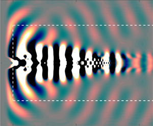
Figure 6. Pressure field associated with the least-stable global mode for  $NPR = 2.10$. The dashed white lines indicate the beginning of the sponge zones; outside these bounds the contours of pressure are only included as a qualitative visualization. The red line indicates Mach wave radiation; the purple line indicates the upstream-propagating acoustic waves.
The normalized coherent fluctuations from the experimental data  $|\boldsymbol {\psi }|$ for the
  $m=0$ jets are presented in figure 7, and for the
  $m=1$ jet in figure 8. The coherent fluctuations are quite similar for the two
  $m=0$ modes, with spatial modulation apparent at both the edges of the shear layer and along the jet centreline. For the
  $m=1$ jet, modulation of the axial velocity component is evident both along the lipline and outside the shear layer, while for the transverse velocity component the strongest modulation occurs along the centreline. A comparison of the fluctuations determined from the least-stable global mode with those associated with the leading POD mode pair is provided in figure 9. Qualitatively, the two results are very similar. The streamwise velocity experiences modulation in the jet core and outside the shear layer for both the global analysis and the experimental data. The transverse velocity is even more closely matched. There are, however, also some key differences: the magnitude of fluctuations in the jet core is higher for the experimental data, and their modulation stronger.

Figure 7. Magnitude of coherent fluctuations for the two jets where the screech mode is an  $m = 0$ azimuthal mode. (a,b) Axial velocity fluctuations. (c,d) Transverse velocity fluctuations.

Figure 8. Magnitude of coherent fluctuations for jet where the screech mode is an  $m = 1$ azimuthal mode. (a) Axial velocity fluctuations. (b) Transverse velocity fluctuations.

Figure 9. Magnitude of fluctuations from both experiment and global analysis. (a,b) Axial velocity fluctuations. (c,d) Transverse velocity fluctuations. All results for  ${NPR} = 2.10$ jet.
While the fluctuations presented in the preceding figures are all associated with fluctuations at a given frequency, these fluctuations can be associated with a broad range of wavenumbers. Consequently, the wavenumber spectra presented in figure 10 are produced by taking the amplitude of (2.6). Phase velocity is defined as  $u_p=\omega / k_x$; as the POD produces modes correlated to the screech phenomenon, here
  $\omega$ is fixed at the screech frequency:
  $\omega = \omega _s$. Thus the sign of
  $k_x$ determines the sign of the phase velocity; here, positive values of
  $k_x$ are associated with a phase velocity in the downstream direction. In this work, we use the sign of the phase velocity as a proxy for the sign of the group velocity. The group velocity determines the direction of energy propagation; waves with negative and positive group velocity may be considered upstream or downstream travelling, respectively. All of the waves in question have phase and group velocities of the same sign in supersonic jets (Towne et al. Reference Towne, Cavalieri, Jordan, Colonius, Schmidt, Jaunet and Brès2017), justifying the assumption made in this analysis. The dashed vertical white lines in figure 10 indicate wavenumbers associated with the ambient speed of sound in the upstream and downstream directions, while the dashed vertical red line indicates the wavenumber associated with the average spacing of the shocks in the flow. All three jets have the majority of the energy concentrated at a wavenumber associated with a phase velocity of
  $u_p \approx 0.7U_j$, with radial structures typical of the classical KH wavepacket, hereafter referred to as the
  $k^{+}_{kh}$ wave. All three jets also have a component with an upstream phase velocity approximately equal to the speed of sound; this is the signature of the guided jet mode previously documented in screeching jets (Edgington-Mitchell et al. Reference Edgington-Mitchell, Jaunet, Jordan, Towne, Soria and Honnery2018; Gojon et al. Reference Gojon, Bogey and Mihaescu2018), hereafter, the
  $k^{-}_{th}$ wave. There is evidence of a third wave at much higher positive wavenumber, observed for all jets, although with different radial structure for the
  $m=1$ case compared to the
  $m=0$ screech modes; this wave will be referred to as the
  $k^{+}_{t}$ wave. The spectrum of the global mode analysis is cleaner than that of the experimental data as shown in figure 11, but the same three structures visible in the experimental data are likewise visible: an upstream-travelling guided jet mode, a downstream-travelling KH wave, and the high-wavenumber mode. The relative amplitudes (normalized against the
  $k^{+}_{kh}$ wave) for both the
  $k^{-}_{th}$ and the
  $k^{+}_{t}$ mode are significantly stronger in the experimental data, but still clearly visible in the global mode. In the global analysis, the wavenumbers for all three waves are approximately
  $\Delta k_{x} D = 0.5$ higher than the corresponding wave in the experimental data.

Figure 10. Wavenumber spectra for all three jets. (a,c,e) Axial velocity fluctuations. (b,d,f) Transverse velocity fluctuations. Note the different  $x$-axis scale for
  ${NPR} = 3.4$.

Figure 11. Wavenumber spectra from both global mode and experiment. (a,b) Axial velocity fluctuations. (c,d) Transverse velocity fluctuations. All results are for the  ${NPR} = 2.10$ jet. Note that a logarithmic contour scale is used in this image.
We return now to the model of Tam & Tanna (Reference Tam and Tanna1982), where it was suggested that the interaction of the KH wavepacket with the stationary shock structures should produce two additional travelling waves in the jet. Due to streamwise variation in the mean flow, the fluctuations associated with the KH wavepacket are spread across a small range of wavenumbers. Likewise, the shock spacing within the jet varies slightly as a function of axial position. Estimates of the wavenumbers associated with both the KH wavepacket and the shock cells are presented in table 3, with a rough estimate of the variation in wavenumber included. We then evaluate (1.4) to produce the two expected wavenumbers (sum and difference) resulting from the interaction between the KH wavepacket and the shock cells. These expected wavenumbers are presented in table 4, along with wavenumbers extracted from the data presented in figure 10. The observed wavenumbers for all the experimental cases and the global analysis fall within the range of expected wavenumbers produced by (1.4). Thus the model of Tam & Tanna (Reference Tam and Tanna1982) provides an explanation for the three wave structures observed in the decomposed experimental data and in the global analysis: one structure is the KH wavepacket, while the other two are waves produced by the interaction between the KH wavepacket and the quasi-stationary shock cells. While the model of Tam & Tanna (Reference Tam and Tanna1982) predicts the wavenumbers of these waves, and provides an explanation for their mechanism of generation, it makes no statement regarding the character of these waves. A cursory examination of figure 10 reveals that each of the three modes has a distinct radial structure. In the following section, we consider the nature of these three waves.
Table 3. Wavenumbers of wave structures.

Table 4. Wavenumber sums and differences.

3.2. The nature of waves in screeching jets
To better characterize the three wave-like structures in the jet, we consider their spatial features: first their axial variation in amplitude and then their radial structure. The spatial amplitude variation associated with the waves is shown qualitatively via the application of a cosine-tapered bandpass filter in the wavenumber domain. The filter has a half-width of  $1.9D$, a taper ratio of
  $0.5$ and is centred on the maximum amplitude for each wave. The results are sensitive to the size and type of the filter; these results should thus only be taken as broadly indicative of peak location and general trends. The amplitude of the fluctuations resulting from this filtering is presented for
  ${NPR} = 2.10$ in figure 12 and for
  ${NPR} = 3.40$ in figure 13. The spatial amplitude distribution of the
  $k^{+}_{kh}$ wavepacket closely resembles the distribution in figures 7 and 8, but without the spatial modulation. This result is unsurprising; the majority of the downstream-travelling energy is associated with the KH wave, and modulation cannot be represented with a single wave. The
  $k^{-}_{th}$ wave peaks at approximately the fourth shock cell for both jets (often observed as the peak sound source location in screeching jets Mercier, Castelain & Bailly Reference Mercier, Castelain and Bailly2017), and as previously discussed in Edgington-Mitchell et al. (Reference Edgington-Mitchell, Jaunet, Jordan, Towne, Soria and Honnery2018) has support outside the shear layer and in the core of the jet. The
  $k^{+}_{t}$ downstream wave reaches maximum amplitude slightly upstream of the peak amplitude location for the upstream wave in the
  ${NPR} = 2.10$ jet, but somewhat further upstream for the
  ${NPR} = 3.40$ jet. The fluctuations associated with this wave are almost entirely bound within the core of the jet. At
  ${NPR} = 2.10$ the amplitude of the axial fluctuations are significantly larger than the transverse; at
  ${NPR} = 3.40$ both transverse and axial fluctuations are observed for the
  $k^{+}_{t}$ wave.

Figure 12. Qualitative amplitude distributions associated with the three wave-like structures for the  ${NPR} = 2.10$ jet (experimental); (a,b)
  $k^{-}_{th}$, (c,d)
  $k^{+}_{kh}$, (e,f)
  $k^{+}_{t}$. (a,c,e) Axial velocity fluctuations, (b,d,f) transverse velocity fluctuations.

Figure 13. Qualitative amplitude distributions associated with the three wave-like structures for the  ${NPR} = 3.40$ jet (experimental); (a,b)
  $k^{-}_{th}$, (c,d)
  $k^{+}_{kh}$, (e,f)
  $k^{+}_{t}$. (a,c,e) Axial velocity fluctuations, (b,d,f) transverse velocity fluctuations.
A comparison of the radial profiles of streamwise velocity for the three identified structures is presented in figure 14, educed from both experiment and global analysis for the  ${NPR} = 2.10$ jet. All curves have been lightly smoothed with a moving average filter to reduce noise; no major features have been removed. The radial structure of the
  $k^{-}_{th}$ wave exhibits a close match between theory and experiment, although the radial decay outside the jet is slower for the global mode. This mismatch in the acoustic field may be a consequence of the PIV measurement being unable to capture weak acoustic perturbations further from the jet. For the
  $k^{+}_{kh}$ wave, the radial structure for both experiment and LSA exhibits the characteristic double peak of a KH wavepacket, with minima at the same radial location, but with a closer spacing between the peaks for the global mode. The radial structure of the
  $k^{+}_{t}$ mode is very similar for the two analyses, although there is a small peak at
  $r/D \approx 0.5$ for the global mode that is larger than that observed in the experiment. As noted earlier, the wavenumber for each of the modes identified in the global analysis is approximately
  $\Delta k_{x} D = 0.5$ higher than the corresponding wave in the experimental data. Since the global analysis is performed on the experimental mean flow, the spacing of the shock cells is the same for both cases. Given this fact, and the slightly higher wavenumber for the KH wave in the global analysis, the increase in wavenumber for the two interaction waves is consistent with the predictions of (1.4).

Figure 14. Radial profiles of streamwise velocity for the three waves discussed in this paper. All waves are normalized to their own maximum value. Results are for the  ${NPR} = 2.10$ jet.
The global analysis has done a remarkable job of capturing the same key structures observed in experiment. Critically, it has demonstrated that it is indeed possible to describe nonlinear KH–shock interactions using a linear model, provided the shock-cell structure is included in the mean flow: the global mode has been shown to correctly capture the nonlinear mechanisms underpinning the production of both upstream- and downstream-travelling waves when coherent turbulent structures are convected through a network of shock cells. It must be noted, however, that the shocks at  $NPR = 2.10$ are very weak, with much of the compression and expansion happening isentropically. How well such linear models will perform as the shocks increase in strength remains an open question. The analysis has also provided some clarification of the nature of the waves that result from this nonlinear interaction. The upstream-travelling wave is the guided jet mode first identified by Tam & Hu (Reference Tam and Hu1989a) as a subsonic instability wave. The downstream wave has not previously been discussed in the context of jet screech, but as will be demonstrated it is simply the downstream-travelling form of the same subsonic wave identified by Tam and Hu, which has recently been the subject of extensive investigation by Towne et al. (Reference Towne, Cavalieri, Jordan, Colonius, Schmidt, Jaunet and Brès2017) and Schmidt et al. (Reference Schmidt, Towne, Colonius, Cavalieri, Jordan and Brès2017). We turn to a local, rather than global, analysis to elucidate the nature of this wave.
Figure 15 presents radial eigenfunctions of the downstream-propagating subsonic instability wave as a function of axial position; these eigenfunctions have been produced via a local analysis on the experimentally derived mean flow at each axial location for the screech frequency  $St=0.67$. In the region of the flow where the shocks are strongest, both the eigenfunction and the wavenumber (omitted for brevity) of this duct-like wave are significantly modulated by the shocks. Despite this modulation, the wave retains its duct-like character: bounded by the shear layer of the jet. In between the shocks, and further downstream, the wave has the typical structure associated with a
  $k^{+}_{t}$ mode of the first radial order, as shown in detail in Towne et al. (Reference Towne, Cavalieri, Jordan, Colonius, Schmidt, Jaunet and Brès2017). Immediately downstream of the shocks, however, the wavenumber of the wave significantly increases, and the peak amplitude shifts from the centreline to almost the edge of the shear layer. Considering the overall characteristics of the shock-cell structure, it is possible that high pressure regions oppose the radial support of these waves in the core, such that the peak is moved to regions of moderate pressure. The eigenfunctions at two selected axial locations are compared with the profile extracted from the experimentally derived wavenumber spectrum. At
  $x/D = 1.3$, the flow is immediately downstream of a shock, and the structure is markedly different to that expected for a
  $k^{+}_{t}$ wave. At
  $x/D = 2.2$, which is close to where the amplitude of this wave peaks according to figure 12, the experiment and stability analysis match well up to
  $r/D \approx 0.5$. The wave is not perfectly trapped by the shear layer in the experimental data, and decays more slowly for
  $r/D > 0.5$.

Figure 15. (a) Eigenfunctions of the  $k^{+}_{t}$ wave as a function of streamwise position, obtained via local linear stability analysis. (b) Comparison of eigenfunctions at two selected axial locations with profile extracted from figure 12. Results for
  ${NPR} = 2.10$ jet.
With the nature of the three waves now established, we can make an overall statement regarding their behaviours. A nonlinear interaction of the KH wavepacket with the shock cells of the jets produces both upstream- and downstream-travelling waves, as predicted by the model of Tam & Tanna (Reference Tam and Tanna1982); this is the first direct experimental validation of the theory, and likewise the first demonstration that a linear global analysis can capture this nonlinear interaction once the shock-cell structure is included in the mean flow. While the model of Tam & Tanna (Reference Tam and Tanna1982) predicted that these waves would exist, it is the mean flow that dictates their nature. In essence, the KH-shock interaction can be thought of as a forcing term, with the response to that forcing dictated by the structure of the mean flow. The mean flow supports upstream- and downstream-travelling waves with distinct radial structures (Tam & Hu Reference Tam and Hu1989a): the  $k^{-}_{th}$ wave has support both inside and outside the jet, while the
  $k^{+}_{t}$ wave is (in a vortex-sheet analysis at least) entirely confined to the core of the jet. Thus, we now have a full explanation for the results presented here: a ‘forcing’ via the mechanism of Tam & Tanna (Reference Tam and Tanna1982), and a response in the form of waves predicted by Tam & Hu (Reference Tam and Hu1989a). In the following section of the paper, we consider the further interaction between these three waves.
3.3. Wave superposition in screeching jets
As alluded to in the introduction of the paper, and demonstrated in figure 7, velocity fluctuations in screeching jets are strongly spatially modulated. In this section we consider possible sources of this modulation. It is already well recognized that the standing wave set up between the downstream-travelling  $k^{+}_{kh}$ waves and the upstream-travelling
  $k^{-}_{th}$ waves results in a periodic modulation of the velocity fluctuations. The effect of this modulation can be removed via the application of a high-pass wavenumber filter with a cutoff at
  $k_x = 0$; all remaining fluctuations are associated with downstream-travelling waves. The results of this filtering are shown in figures 16 and 17; all periodic modulation of velocity fluctuations outside of the jet lipline have been removed, but all three jets still exhibit periodic modulation within the jet core. For the
  $m=0$ screech cases, there is a periodic oscillation of axial velocity fluctuation amplitude in the jet core, but relatively little modulation of the transverse velocity component. For the helical screech mode, there remains significant modulation of velocity in both the axial velocity (primarily on the high-speed side of the shear layer) and the transverse velocity (at the centreline).

Figure 16. Magnitude of coherent fluctuations with positive phase velocity for the two jets where the screech mode is an  $m = 0$ azimuthal mode. (a,b) Axial velocity fluctuations. (c,d) Transverse velocity fluctuations.

Figure 17. Magnitude of coherent fluctuations with positive phase velocity for jet where the screech mode is an  $m = 1$ azimuthal mode. (a) Axial velocity fluctuations. (b) Transverse velocity fluctuations.
Given the restriction of this modulation to the core of the jet, one candidate is a superposition of the  $k^{+}_{kh}$ wave with the trapped
  $k^{+}_{t}$ waves. To examine superposition between all three waves, dual-peak bandpass filters are applied to each of the three possible wave–wave combinations, with both the filtered-wavenumber spectra and resultant amplitude plots presented in figures 18 and 19. Again, it must be emphasized that information is lost in this filtering process, and the results should only be considered a qualitative indication. As such, amplitudes have been normalized by the maximum amplitude in each case for clarity, although the fluctuations resulting from the superposition of the
  $k^{-}_{th}$ and
  $k^{+}_{t}$ waves is an order of magnitude weaker than all others. As expected, the superposition of the
  $k^{-}_{th}$ and
  $k^{+}_{kh}$ produces the familiar standing-wave pattern in the near field of the jet, but is also responsible for significant modulations within the core of the jet. The
  $k^{-}_{th}$ and
  $k^{+}_{t}$ superposition is highly periodic and confined to the core of the jet, but is very weak and contributes minimally to the overall fluctuations. The
  $k^{+}_{t}$ and
  $k^{+}_{kh}$ wave superposition, while weaker than that of the
  $k^{-}_{th}$ and
  $k^{+}_{kh}$, still results in a significant spatial modulation of velocity fluctuation. As the
  $k^{+}_{t}$ is confined within the lipline of the jet, so too is the spatial modulation of velocity; outside the jet it is only the superposition of the
  $k^{-}_{th}$ and
  $k^{+}_{kh}$ waves that produces spatial modulation. In the flows we consider here, both the
  $k^{-}_{th}$ and
  $k^{+}_{t}$ waves result from a nonlinear interaction between the
  $k^{+}_{kh}$ wavepacket and the shocks. The superposition of the
  $k^{+}_{kh}$ wave with these two new waves thus produces a spatial modulation whose wavelength closely matches the shock spacing in the flow.

Figure 18. Interaction between pairs of waves for  $\textit {NPR} = 2.10$ jet, represented through streamwise velocity fluctuations. (a–c) Wavenumber spectra. (d–f) Velocity fluctuation amplitude (normalized).

Figure 19. Interaction between pairs of waves for  ${NPR} = 3.40$ jet, represented through streamwise velocity fluctuations. (a–c) Wavenumber spectra. (d–f) Velocity fluctuation amplitude (normalized).
Plots of centreline fluctuation amplitude are presented in figure 20. If it is assumed that the bandpass filters only admit fluctuations associated with these waves, then even on the centreline, the majority of the modulation is evidently derived from the superposition of the  $k^{-}_{th}$ and
  $k^{+}_{kh}$ waves, with the superposition of the
  $k^{+}_{t}$ and
  $k^{+}_{kh}$ providing a small but non-negligible contribution. When the superposition of all three waves is considered, the modulation in the range
  $2 \leqslant x/D \leqslant 4$ is reproduced almost perfectly; outside this range the growth and decay requires the inclusion of lower wavenumbers than those admitted by the filter. There is, however, a serious limitation with this analysis; even in the absence of either the
  $k^{-}_{th}$ or the
  $k^{+}_{t}$ waves, any modulation of the
  $k^{+}_{kh}$ waves would be contained in wavenumbers
  $k^{+}_{kh}-k_s$ and
  $k^{+}_{kh}+k_s$. These are of course the same wavenumbers occupied by the
  $k^{-}_{th}$ and
  $k^{+}_{t}$ waves. While outside of the shear layer, it seems clear that the majority of observed modulation arises from the previously identified ‘standing wave’ formed by the
  $k^{+}_{kh}$ and
  $k^{-}_{th}$, within the jet core it is difficult to decouple modulation of the overall fluctuations due to wave superposition from modulation of the
  $k^{+}_{kh}$ by the shock. Preliminary local stability calculations presented in Edgington-Mitchell et al. (Reference Edgington-Mitchell, Duke, Wang, Harris, Schmidt, Jaunet, Jordan and Towne2019) suggested that the influence of the shocks on the growth rate of the
  $k^{+}_{kh}$ wave were minimal, but a deeper analysis using stability tools is required to provide a categorical answer to the question of wave modulation in the core of shock-containing jets.

Figure 20. Centreline streamwise velocity fluctuation profiles for filtered data subsets of  ${NPR} = 2.10$ jet.
4. Conclusion
Tam & Tanna (Reference Tam and Tanna1982) first suggested that the interaction of the KH wavepacket with the shocks in a supersonic jet would produce waves with both positive and negative phase velocity. Here, we have provided the first evidence for these waves in the velocity field of screeching supersonic jets across a range of operating conditions. Further, we have demonstrated that the radial structure of these waves is dictated by the base flow, in accordance with the waves predicted by Tam & Hu (Reference Tam and Hu1989a) via a vortex-sheet model. The upstream-travelling wave has support both inside and outside the jet, while the downstream-travelling wave is confined within the core of the jet. This downstream wave is the ‘trapped’ wave described in Towne et al. (Reference Towne, Cavalieri, Jordan, Colonius, Schmidt, Jaunet and Brès2017), that treats the jet like a soft-walled duct. The presence of these waves has been demonstrated for three different stages of jet screech, with shocks ranging from relatively weak to quite strong. Thus we suggest that as long as the mean flow is able to support these waves, they should be expected in all stages of jet screech, irrespective of shock strength.
We have also demonstrated that the nonlinear wave interaction can be captured by a linear global analysis performed on the experimentally derived mean flow, thanks to the presence of the shock-cell structure in the mean flow. Despite the many nonlinear mechanisms active in a screeching jet, the linear analysis predicts the correct screech tone to within  ${\approx }1\,\%$, and the same three wave structures observed in experiment are likewise evident in the global mode. This suggests that, aside from the nonlinear wave interaction that drives the upstream- and downstream-travelling waves, the remaining frequency-selection mechanisms (propagation characteristics of the
  $k^{+}_{kh}$ and
  $k^{-}_{th}$ waves, receptivity in the nozzle plane) are linear. As a cautionary note, however, it must be emphasized that this result has only been demonstrated for the case with the weakest shocks.
Finally, the superposition of these three wave structures and the spatially modulated velocity fluctuations that result were considered. Outside of the jet, no modulation is evidence once upstream-travelling waves are excluded, consistent with prior work suggesting this modulation is due to interaction between the downstream-propagating and upstream-propagating waves. In the core of the jet the result is less clear; some amount of modulation will be due to the two waves generated from the interaction, but the present analysis is unable to decouple this from any direct influence that the shocks have on the KH wavepacket.
Funding
D.E.-M. and P.N.'s contributions to this work were funded by the Australian Research Council under the Discovery Project scheme via DP190102220.
Declaration of interests
The authors report no conflict of interest.
Appendix. Sensitivity of Reynolds number in global stability analysis
Considering that the Reynolds number chosen for the global stability analysis differs from the experimental one, and that no turbulent viscosity model is used, it is useful to analyse the influence of this parameter on the prediction of the screech frequency and on the shapes of the modes. Here, the Reynolds number was varied in the interval  $[2500 \ 30\,000]$, and the frequencies of the screech mode (analysed in § 3.1) and the respective growth rates are shown in figure 21. These results show the robustness of the prediction regarding this parameter: the variation of the Strouhal number is only of the order of
  $10^{-3}$ over this range of Reynolds numbers. Also, the growth rate of the screech mode increases as this parameter is increased, as expected in this sort of stability analysis (see Coenen et al. (Reference Coenen, Lesshafft, Garnaud and Sevilla2017), for instance). Interestingly, the mode does not cross the real axis, and remains stable for all Reynolds numbers analysed. This may be due to the low shock-cell strength for the present case, or even due to the absence of the nozzle in the computational domain.

Figure 21. Strouhal number of the screech mode (a) and the respective growth rate (b) as functions of Reynolds number, from global stability analysis.
The shapes of the modes (represented by the real part of the streamwise velocity) for the different Reynolds numbers are shown in figure 22. Overall, all mode shapes are qualitatively similar to the leading POD mode shown in figure 5. For low Reynolds numbers, the increased viscosity leads to modes that are spatially smoother, especially around the shear layer. The streamwise and radial variation are also slower, which leads to more spatially spread mode shapes. As the Reynolds number is increased, the modes start to become more concentrated around the shear layer, and the spatial changes are steeper. The high similarity between the low Reynolds number mode and the POD mode can be associated with the action of the turbulent viscosity in this flow: since such a model is not used in the present analysis, a consideration of a lower Reynolds number can partially account for the increased turbulent mixing in the linear analysis, as shown by Pickering et al. (Reference Pickering, Rigas, Schmidt, Sipp and Colonius2020).

Figure 22. Shapes of the modes for different values of Reynolds number from global stability analysis. Only the real part of the streamwise velocity is shown.


