


1. Introduction
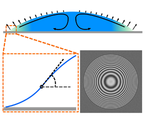
Evaporation of a sessile droplet, a simple object comprising all the complexities of the phenomena such as wettability, contact-line dynamics, Marangoni flows, deposition patterns, phase change, etc., has attracted considerable attention over the last few decades (Lohse & Zhang Reference Lohse and Zhang2020) because of its connection with a wide variety of applications such as inkjet printing (Tekin, de Gans & Schubert Reference Tekin, de Gans and Schubert2004; Singh et al. Reference Singh, Haverinen, Dhagat and Jabbour2010; Siregar, Kuerten & van der Geld Reference Siregar, Kuerten and van der Geld2013), spray cooling (Kim Reference Kim2007), thin film deposition (Kim et al. Reference Kim, Jeong, Park and Moon2006), DNA control (Jing et al. Reference Jing1998; Dugas, Broutin & Souteyrand Reference Dugas, Broutin and Souteyrand2005), disease diagnostic tool (Yakhno et al. Reference Yakhno, Sedova, Sanin and Pelyushenko2003) and control of motion of small quantities of liquids (Cira, Benusiglio & Prakash Reference Cira, Benusiglio and Prakash2015). Evaporative cooling can lead to Marangoni flows due to temperature gradients (Savino, Paterna & Favaloro Reference Savino, Paterna and Favaloro2002; Hu & Larson Reference Hu and Larson2005; Xu & Luo Reference Xu and Luo2007; Barmi & Meinhart Reference Barmi and Meinhart2014), affecting the droplet shape (Xu et al. Reference Xu, Zhang, Yang and Vest1984; Tsoumpas et al. Reference Tsoumpas, Dehaeck, Rednikov and Colinet2015). When dealing with multicomponent droplets, especially not highly volatile, control is rather assumed by the solutal Marangoni stresses (Cira et al. Reference Cira, Benusiglio and Prakash2015), arising due to non-uniform vaporization of the components. Depending on their direction (towards the contact line or towards the apex of the droplet), they can either enhance spreading (Carles & Cazabat Reference Carles and Cazabat1989; Cira et al. Reference Cira, Benusiglio and Prakash2015; Keiser et al. Reference Keiser, Bense, Colinet, Bico and Reyssat2017; Parimalanathan et al. Reference Parimalanathan, Dehaeck, Rednikov and Colinet2021), or make for a quasi-steady ‘contracted’ droplet (Cira et al. Reference Cira, Benusiglio and Prakash2015; Karpitschka, Liebig & Riegler Reference Karpitschka, Liebig and Riegler2017; Benusiglio, Cira & Prakash Reference Benusiglio, Cira and Prakash2018; Parimalanathan et al. Reference Parimalanathan, Dehaeck, Rednikov and Colinet2021) similar to what was observed with a thermal Marangoni effect (Tsoumpas et al. Reference Tsoumpas, Dehaeck, Rednikov and Colinet2015). For instance, a droplet of water and propylene glycol (PG) mixture on a high energy surface and at a not so large ambient humidity manifests a contracted shape with an apparent contact angle roughly of the order of 10 $^{\circ }$ (Cira et al. Reference Cira, Benusiglio and Prakash2015; Karpitschka et al. Reference Karpitschka, Liebig and Riegler2017; Benusiglio et al. Reference Benusiglio, Cira and Prakash2018), while droplets of pure water or pure PG would totally spread (perfect wetting). Indeed, the higher volatility of water makes for a relative water depletion near the contact line (where the liquid film is thinner and the evaporation rate is higher). Such depletion was directly measured by Kim & Stone (Reference Kim and Stone2018). As a consequence, the surface tension is lower at the contact line (water possessing higher surface tension than PG). Therefore, the solutal Marangoni stresses pump towards the apex, hence a contracted droplet (cf. figure 1). It is also principally due to the solutal Marangoni effect that such sessile droplets are set into motion in the direction of an ambient humidity gradient (Cira et al. Reference Cira, Benusiglio and Prakash2015).

Figure 1. Sketch of the phenomenon. Going from darker (blue) to lighter (tints of cyan) shading symbolizes a decrease in water content.
Cira et al. (Reference Cira, Benusiglio and Prakash2015) and Benusiglio et al. (Reference Benusiglio, Cira and Prakash2018) were the first to put into evidence and measure the apparent contact angles of such water–PG droplets, which are also the subject of the present paper. They built an heuristic model of the phenomenon. For droplets of a larger volume, a comprehensive amount of measurement data for a number of water–diol pairs (including water–PG) is due to Karpitschka et al. (Reference Karpitschka, Liebig and Riegler2017). All data were captured by means of a universal modelling-assisted fit in the form of a power law for the relative humidity deviation from its equilibrium value, the prefactor depending on the diol mass fraction in the liquid. Their more rigorous and comprehensive modelling highlights most notably PG segregation and a consequent regularization of an otherwise diverging evaporation flux towards the contact line. However, in our understanding, Karpitschka et al. (Reference Karpitschka, Liebig and Riegler2017) did not attempt a direct quantitative comparison of their theory with experiment. We were unable to find the material properties such as the viscosity and diffusion coefficient used in the computations. Their species transport equation does not contain what we here refer to as the mixing in the droplet by means of the solutal Marangoni flow, the importance of which was pointed out by Charlier et al. (Reference Charlier, Rednikov, Dehaeck, Colinet and Terwagne2019) and Charlier (Reference Charlier2020). We have recently become aware of a study by Ramírez-Soto & Karpitschka (Reference Ramírez-Soto and Karpitschka2021) essentially incorporating the Marangoni mixing into a model akin to Karpitschka et al. (Reference Karpitschka, Liebig and Riegler2017). Similarly to Charlier et al. (Reference Charlier, Rednikov, Dehaeck, Colinet and Terwagne2019) and Charlier (Reference Charlier2020), this is accomplished by means of the Taylor dispersion. Ramírez-Soto & Karpitschka (Reference Ramírez-Soto and Karpitschka2021) also provide a direct experimental measurement of the solutal Marangoni flow, which is directed towards the centre at the droplet surface as expected.
In the present paper, we expose a specific morphology consisting of the existence of a distinguished narrow region at the foot of the droplet and relate it to the apparent contact angles and Marangoni mixing. On the experimental side (§ 2), our interferometric methods (Dehaeck, Tsoumpas & Colinet Reference Dehaeck, Tsoumpas and Colinet2015; Dehaeck & Colinet Reference Dehaeck and Colinet2016) enable us to resolve the slope and height profiles of the droplet in the foot region. There, we clearly disclose a maximum-slope (shape-inflection) point in a close vicinity of the contact line (cf. figure 1), the maximum slope values being associated with the apparent contact angles. A series of measurements are carried out at various droplet compositions (PG fractions) and ambient relative humidity values.
On the theoretical side (§ 3), we go straight to a local modelling of the foot region and the apparent contact angles of a solutal Marangoni nature generated therein. This is accomplished on the premise of a scale separation between the foot region and the core of the droplet (the latter supposed to adhere to the classical static shape, Allen (Reference Allen2003)), which is supported by the observation. The Marangoni mixing in the liquid is accounted for in the model, by means of the Taylor dispersion. We start from a particularly simple model, reducing to a system of ordinary differential equations (ODEs), but capturing the essence of the phenomenon and highlighting the scales and the dependence on the material properties. In particular, we thereby observe a crucial role of the Marangoni mixing for the scale separation and self-consistency of the local approach. One further step of generalization, still in the framework of a local approach in the foot region, is undertaken at the end of § 3. This is required for a better comparison with experiment, in a wider parameter range. Such a comparison, with our own experimental results as well as those by Cira et al. (Reference Cira, Benusiglio and Prakash2015), Benusiglio et al. (Reference Benusiglio, Cira and Prakash2018) and Karpitschka et al. (Reference Karpitschka, Liebig and Riegler2017), is discussed more thoroughly in § 4.
Finally, the developed experimental and theoretical tools are applied to study the attraction of droplets by a nearby humidity source (§ 5). Thus, the interferometry permits us to disclose the associated induced asymmetry of the sessile droplet; the contact angles calculated as a function of the ambient humidity (among other parameters) permit us to deal with the droplet behaviour in a humidity gradient from the source. Certain mathematical details are relegated to appendices. The conclusions are summarized in § 6.
2. Experimental
Binary-liquid sessile droplets of distilled water and PG (‘AMRESCO’ high purity grade PG) of a volume  ${\sim }0.5\,\mathrm {\mu }$L, prepared at different volume fractions using a ‘VWR Signature EHP Pipettor’ pipette, were deposited at room temperature in the ambient atmosphere on a glass slide (
 $76\,\textrm {mm}\times 26\,\textrm {mm}\times 1\,\textrm {mm}$). Before first use, slides were washed using ethanol, acetone and distilled water, which was followed by plasma cleaning (four minutes with ‘CUTE FEMTO SCIENCE’ V2.0). After first use, glass slides were washed only with distilled water before plasma cleaning. Ambient temperature and relative humidity were measured using a ‘Lufft OPUS 20’ weather station. The relative humidity values we worked at were either due to weather conditions, or (for higher values) were achieved by boiling water in the laboratory. We here study the quasi-steady contracted shapes, with finite apparent contact angles
  $\theta _{app}$, the droplets attain shortly after the deposition in spite of perfect wetting of each of the components. (For pure water droplets, small finite contact angles (
 ${\lesssim }3^\circ$, generally well smaller than
  $\theta _{app}$ here) could nonetheless be observed, which we attribute to the evaporation-induced contact angle (cf. e.g. Poulard et al. Reference Poulard, Guéna, Cazabat, Boudaoud and Ben Amar2005; Pham et al. Reference Pham, Berteloot, Lequeux and Limat2010; Colinet & Rednikov Reference Colinet and Rednikov2011; Morris Reference Morris2014; Rednikov & Colinet Reference Rednikov and Colinet2019, Reference Rednikov and Colinet2020), and not the Young's angle.) The runs with any detected pinning of the contact line were discarded. A Mach–Zehnder interferometer, using a helium–neon laser, allows us to extract the local slopes of the droplet at every point (Dehaeck et al. Reference Dehaeck, Tsoumpas and Colinet2015; Dehaeck & Colinet Reference Dehaeck and Colinet2016) starting from interferometric images as outlined in figure 2. To complete this procedure, refractive indexes of the binary liquid of different volume fractions were preliminarily measured using an ‘ATAGO’ refractometer DRA1 (see Appendix A).

Figure 2. (a) Typical interference pattern of a water–PG droplet before treatment. Circles on the drop are aliasing artefacts. Only the interference pattern centred on the droplet is physical. (b) Same figure after treatment. Colour is linked to the local slope in degrees. The red solid line is the single slice we consider to obtain the slope profile below. (c) Extracted slope profile. The lengths are in pixels ( $2.6\,\mathrm {\mu }$m per pixel). Droplet volume
  $V = 0.5\,\mathrm {\mu }$L, contact radius
  $R=1.55$ mm, ambient relative humidity 54 % (
 $R\!H = 0.54$), temperature
  $T = 20\,^{\circ }\mathrm {C}$, 50 % PG volume fraction in the liquid (
 $c_m\approx 0.5$).
The thereby measured slope profiles are illustrated in figure 3. An interesting feature of the slope profiles is that they reach a maximum value  $\theta _{max}$ (the inflection point of the height profile) generally very close to the contact line (of the order of tens of
  $\mathrm {\mu }$m in the most drastic cases). Then the slope is seen to decrease again, apparently to meet the surface at a microscopic contact angle
  $\theta _{mic}$, although we here do not claim any reliable measurement of
  $\theta _{mic}$ in view of a possible loss of resolution and do not pursue this issue any further. The classical static shapes (Allen Reference Allen2003)
 \begin{equation} h=\theta_{app} l_c \frac{I_0\left(\dfrac{R}{l_c}\right)-I_0\left(\dfrac{r}{l_c}\right)}{I_1 \left(\dfrac{R}{l_c}\right)},\quad V={\rm \pi} \theta_{app} l_c R^2 \frac{I_2\left(\dfrac{R}{l_c}\right)}{I_1\left(\dfrac{R}{l_c}\right)}, \end{equation}
with  $h$ the liquid thickness,
  $r$ the radial coordinate,
  $R$ the droplet contact radius,
  $V$ the droplet volume,
  $l_c=\sqrt {\gamma /\rho _l g}$ the capillary length,
  $\gamma$ the surface tension,
  $\rho _l$ the liquid density,
  $g$ the gravity acceleration,
  $I_0$ ,
  $I_1$ and
  $I_2$ the modified Bessel functions, represent well the main part of the droplet (solid lines of figure 3). For the droplet sizes considered here (
 $R< l_c$), they are close to just the spherical caps
  $h=({\theta _{app}}/{2 R}) (R^2-r^2)$ (with
  $V= \frac{\rm \pi}{4} \theta _{app} R^3$). However, they fail to predict the narrow high-curvature zone of the foot of the droplet around the maximum-slope (shape-inflection) point. Obviously, in view of the narrowness of that zone,
 \begin{equation} \theta_{app}\approx \theta_{max}, \end{equation}
although distinctions between various possible finer definitions of  $\theta _{app}$ as well as a finer distinction between
  $\theta _{app}$ and
  $\theta _{max}$ can in principle be drawn. One of such finer distinctions will be required at a later stage, but they are disregarded for the moment.

Figure 3. Examples of measured droplet slope profiles. Classical static shape fits over the core of the droplet (solid lines).  $V = 0.4\pm 0.07\,\mathrm {\mu }$L, relative humidity 51 % (
 $R\!H = 0.51$),
  $T = 20\,^{\circ }\mathrm {C}$, 10 %, 40 % and 70 % PG volume fractions in the liquid (
 $c_m\approx 0.9, 0.6\ \text {and}\ 0.3$, respectively).
One can already notice in figure 3 a non-monotonic dependence of  $\theta _{max}$ on PG concentration, which tendency can be observed in figure 4 in a more global context. In this latter figure, the measured angles
  $\theta _{max}$ are shown with symbols as a function of PG concentration for different ambient relative humidity values together with some other similar results from the literature, which are seen to agree well with our own measurements. The curves correspond to theoretical results that will be explained in the following sections. At a given humidity, the largest values of
  $\theta _{max}$ are attained for intermediate PG concentrations. The angles decrease both towards the pure water limit and towards what appears as the equilibrium concentration (corresponding to the liquid water content in equilibrium with the vapour at a given ambient humidity, see also later on). These tendencies go along with the expected key roles of both the solutal Marangoni effect (vanishing for pure water) and the evaporation (vanishing at the equilibrium concentration). Furthermore, the angles are seen to decrease with the humidity, which is understandable in view of the expected similar tendency for the evaporation rates. Beyond the equilibrium concentration, the droplet enters into a spreading regime (replacing the contraction one studied here), but this is already outside the scope of the present paper.

Figure 4. Contact angle results for  ${\sim }0.5\,\mathrm {\mu }$L droplets. Experimental data from Cira et al. (Reference Cira, Benusiglio and Prakash2015) and Benusiglio et al. (Reference Benusiglio, Cira and Prakash2018) (unfilled symbols) and our own
  $\theta _{max}$ data (filled symbols) at
  $\sim$20
  $^{\circ }$C. Ultimate predictions of
  $\theta _{max}$ by our model (solid lines), cf. the rectified local model later on.
3. Theoretical
3.1. Basic assumptions
The theoretical approach is based on the following premises.
We consider a sessile droplet composed of water and PG and evaporating into ambient air at a relative humidity  $R\!H$. The problem is axisymmetric (although this assumption will partly be overridden in § 5 by considering a gradient of
  $R\!H$).
As the contact angles and film slopes are here not large ( ${<}20^\circ$), we rely upon the lubrication approximation in the liquid phase (inside the droplet). The composition variation across the droplet is neglected.
The experimental results (figure 3) permit us to conjecture that, shape-wise, the solutal Marangoni action is immediately essential just in a small vicinity of the contact line (foot region), setting off the apparent contact angle for the classical static shape (2.1a) in the core of the droplet. Accordingly, assuming such a separation of scales, we here advance a local approach/model intended to be valid in the foot region and match (2.1a).
We further conjecture (to be verified a posteriori) that, for such a strong localization in the foot region, there must be a good solutal-Marangoni mixing inside the droplet, which will smooth out concentration gradients in the core of the droplet and (to a lesser extent) in the foot region. Accordingly, we assume that the water mass fraction  $c(r)$ deviates everywhere only slightly from its (spatially quasi-constant) value
  $c_m$ in the core of the droplet:
 \begin{equation} c=c_m+c'(r) \quad (c'\ll 1). \end{equation}
The mixing will here be treated by means of the Taylor dispersion (Taylor Reference Taylor1953, Reference Taylor1954) in the framework of the lubrication approximation.
Only quasi-steady regimes are considered. In particular, an initial fast-spreading stage (upon the droplet deposition) is assumed to be over. The strong mixing and localization also favour fast attaining a quasi-steady state from the viewpoint of concentration distribution, so that the composition  $c_m$ has not yet changed significantly due to evaporation, as compared with the initial one upon the droplet deposition. (In fact, one can refer to figure 1(c) of a recent preprint by Ramírez-Soto & Karpitschka (Reference Ramírez-Soto and Karpitschka2021) to appreciate how fast the quasi-steadiness is really reached (in less than
  $1\,\mathrm {s}$).) Thus,
  $c_m$ is here treated as an input parameter, identified with the initial composition. The other input parameters (apart from the material properties) are the droplet size (represented by either the droplet contact radius
  $R$, or the droplet volume
  $V$) and the ambient relative humidity
  $R\!H$ (expressed either in fraction terms or in per cent as evident from the context).
A direct contribution of evaporation into the flow inside the droplet is neglected with respect to the solutal Marangoni flow. The apparent contact angles are assumed to be entirely associated with the latter.
The material properties of the liquid such as the surface tension  $\gamma (c)$,
  $({\textrm {d}\gamma }/{\textrm {d} c})(c)$, diffusion coefficient
  $D_l(c)$ and dynamic viscosity
  $\eta (c)$ are all functions of the composition. These dependencies are fully accounted for in the present paper using results from the literature (cf. Appendix A). However, by virtue of the ansatz (3.1), they are here evaluated at
  $c=c_m$ and otherwise treated as constants.
In view of close densities of water and PG, we shall adopt an approximate constant value of the liquid density throughout,  $\rho _l\approx 1015\,\mathrm {kg}\,\mathrm {m}^{-3}$, also implying no distinction between the mass and volume fractions. The PG volume fraction (used in figure 4) is then
  $(1-c_m)\times 100\,\%$. Neglecting the natural convection inside the droplet is, notwithstanding, a separate assumption, adopted in view of small contact angles (cf. Diddens, Li & Lohse Reference Diddens, Li and Lohse2021).
The volatility of PG is neglected. As for water, Raoult's law is assumed at any liquid composition, which use is supported by data from Verlinde, Verbeeck & Thun (Reference Verlinde, Verbeeck and Thun2010) and Karpitschka et al. (Reference Karpitschka, Liebig and Riegler2017, figure S2).
Droplet evaporation is controlled by vapour diffusion in the gas. The vapour is dilute (hence no Stefan flow), given that the saturation pressure of water is much smaller than the atmospheric pressure at the temperatures considered ( ${\sim }20\,^\circ$C). In view of the small slopes, the droplet is approximated by a flat disk from the viewpoint of the vapour diffusion problem in the gas. By virtue of the ansatz (3.1), the distribution of the evaporation flux density
  $j(r)$ (in
  $\mathrm {kg}\,\mathrm {m}^\mathrm {-2}\,\mathrm {s}^\mathrm {-1}$) along the droplet diameter is assumed to be the one for a droplet of a uniform composition
  $c=c_m$, neglecting a feedback from
  $c'(r)$. This gives rise to a well known expression (e.g. Popov Reference Popov2005)
 \begin{equation} j(r)=\frac{2 D_g\rho_{sat} (\chi_m-R\!H)}{{\rm \pi} \sqrt{R^2-r^2}} \end{equation}
with  $D_g=2.55\times 10^{-5}\,\textrm {m}^2\,\textrm {s}^{-1}$ the water vapour diffusivity and
  $\rho _{sat}=0.017\,\textrm {kg}\,\textrm {m}^{-3}$ (at 20
  $^{\circ }$C) the saturation density of water vapour, except that it is here modified by a prefactor
  $(\chi _m-R\!H)$ accounting for Raoult's law and the ambient humidity. The molar fraction of water in the liquid
  $\chi$ is related to
  $c$ by
 \begin{equation} \chi=\frac{M_{pg} c}{M_{pg} c+ M_w (1-c)},\quad \chi_m=\frac{M_{pg} c_m}{M_{pg} c_m+ M_w (1-c_m)} \end{equation}
(likewise for  $\chi _m$ versus
  $c_m$), where
  $M_w=18\,\textrm {g}\,\textrm {mol}^{-1}$ and
  $M_{pg}=76\,\textrm {g}\,\textrm {mol}^{-1}$ are the molar masses of water and PG, respectively. The prefactor and the evaporation flux (3.2) both vanish at equilibrium. The equilibrium relative humidity
  $R\!H_{eq}$ for a given liquid composition
  $\chi _m$ is then obviously
  $R\!H_{eq}=\chi _m$. Inversely, for a given
  $R\!H$ the equilibrium composition
  $\chi _{m,{eq}}$ corresponds to
  $\chi _{m,{eq}}=R\!H$. In the present paper, we study the case
  $\chi _m>R\!H$ (in other words,
  $\chi _m>\chi _{m,{eq}}$, or
  $R\!H< R\!H_{eq}$), when, as argued in § 1, the evaporation and the solutal Marangoni stresses due to the ensuing composition inhomogeneity make for a contraction regime of the droplet. Note in (3.2) a well known integrable divergence of the evaporation flux at the contact line (as
  $r\to R$).
In the narrow foot region near the contact line, for which our local model will be developed, the evaporation flux (density) distribution can be established as the edge behaviour ( $x\equiv R-r$,
  $x\ll R$) within (3.2):
 \begin{equation} j(x)=\frac{\sqrt{2}D_g\rho_{sat}}{\rm \pi}\frac{1}{\sqrt{R x}} (\chi_m-R\!H). \end{equation}
The local model based upon (3.4) and thus neglecting a feedback between  $j(x)$ and
  $c'(x)$ (cf. above (3.2)) will be referred to as the ‘non-rectified’ local model. In contrast, the ‘rectified’ local model will be the one fully accounting for the mentioned feedback (‘rectification’) and yielding a substitute to (3.4) to be considered later on. Regardless, even in the latter case, it will still be assumed that the ‘non-rectified’ expression (3.2) is valid, although just in the core of the droplet (excluding the foot region). This is justified by an expected higher degree of mixing and composition uniformity in the core of the droplet and a higher degree of water depletion (larger values of
  $-c'$) in the foot region. Thus, the rectification will thereby just stay confined to the local problem in the foot region.
The rationale behind considering the non-rectified local model (despite the eventual availability of a more general, rectified one here) is its incomparable simplicity, which will permit us to probe the essence of the phenomenon in a more subtle and clear way. Furthermore, the non-rectified approach can already prove sufficient at least in certain cases. For instance, one can expect it to work for droplets with a large water content, when close to the pure-water case. At the same time, it will prepare ground for passing to the rectified local model should the need arise. In the remainder of the present section, the developments of §§ 3.2, 3.3 and 3.6 equally apply to both local models. The consideration in §§ 3.4, 3.5, 3.7 and 3.8 is based on the non-rectified approach, although the discussion in §§ 3.5 and 3.7 is deemed to be pertinent regardless of the model type. Finally, the rectified local model is tackled in § 3.9.
3.2. Formulation
We now focus on the liquid film in the foot region. Within the lubrication approximation, the problem is described by two dependent variables, which are the height  $h(x)$ and concentration
  $c'(x)$ distributions along the film (Cartesian coordinate
  $x>0$ with
  $x=0$ chosen at the contact line). Therefore, two equations need to be formulated (momentum and species conservation), which are considered in the following two paragraphs.
With no slip at the substrate ( $z=0$) and the solutal Marangoni stress at the free surface
  $z=h$, the solution of the momentum equation
  $0=-\partial _x p+\eta \partial _{zz} u$ for the velocity field component parallel to the substrate in the lubrication approximation is
 \begin{equation} u=\eta^{{-}1} (\partial_x p) \left(\frac{1}{2} z^2-h z\right)+\eta^{{-}1} \frac{\textrm{d}\gamma}{\textrm{d} c} (\partial_x c') z, \end{equation}
a sum of the (half-) Poiseuille and linear shear flows. Here  $z$ is the Cartesian coordinate across the film, and
  $p=-\gamma \partial _{xx} h$ the Laplace pressure (gravity being negligible in this small region). With the evaporation-related flow neglected as stated in § 3.1, a quasi-steady lubrication equation merely reduces to
  $\int _0^h u\,\textrm {d} z=0$, and hence
 \begin{equation} \gamma h \partial_{xxx} h +\frac{3}{2}\frac{\textrm{d}\gamma}{\textrm{d} c}\partial_x c'=0. \end{equation}
According to (3.6), the film is shaped by the solutal Marangoni effect moderated by the capillary pressure.
We next turn to an equation for  $c'(x)$. We recall (cf. § 3.1) that the dependence of
  $c'$ on
  $z$ is neglected to leading approximation assuming a good levelling by molecular diffusion in our thin droplet, hence
  $c'=c'(x)$. The water species balance in any element
  ${\textrm {d}\kern0.06em x}$ of the film consists of a diffusion influx
  $h\rho _l D_{eff}\partial _x c'\vert _x^{x+{\textrm {d}\kern0.06em x}}$, convective suction influx
  $j c_m\,{\textrm {d}\kern0.06em x}$ (here neglecting
  $c'$ against
  $c_m$, cf. § 3.1) due to the overall evaporation flux
  $j(x)$ (in
  $\textrm {kg}\,\textrm {m}^{-2}\,\textrm {s}^{-1}$), and losses
  $(-j_w\,\textrm {d}\kern0.06em x)$ due to water evaporation flux
  $j_w(x)$ (in
  $\textrm {kg}\,\textrm {m}^{-2}\,\textrm {s}^{-1}$). In a quasi-steady state, the sum of the three must vanish. As water is considered as the only volatile component in a water–PG mixture, and hence
  $j_w=j$, we arrive at the following equation:
 \begin{equation} \partial_x (h D_{eff} \partial_x c')- j(1-c_m)/\rho_l=0, \end{equation}
according to which the concentration profile is a result of the competition between the evaporation and diffusion. A more general outlook on (3.6) and (3.7) can be found in Appendix B. Here  $D_{eff}$ is the effective diffusion coefficient resulting from the Taylor dispersion (Taylor Reference Taylor1953, Reference Taylor1954; Van den Broeck Reference Van den Broeck1990). The idea behind this is that the combination of molecular diffusion
  $D_l$ along
  $z$ and a flow
  $u(z)$ with
  $\int _0^h u\,\textrm {d} z=0$ (as here) results in an additional diffusion-like smearing of the profile
  $c'(x)$. Hence the form
  $D_{eff}=D_l (1+B P\!e^2)$, where
  $B$ is a numerical coefficient and
  $P\!e$ a Péclet number. Proceeding in a standard way, one can obtain
  $BP\!e^2=(D_l^2 h)^{-1} \int _0^h (\int _0^z u(z')\,\textrm {d} z' )^2 \,\textrm {d} z$. Using
  $u(z)$ from (3.5) and using (3.6) as a constraint, one finally arrives at
 \begin{equation} D_{eff}= D_l \left[1+\frac{1}{1680} \left(\frac{1}{D_l\eta} \frac{\textrm{d}\gamma}{\textrm{d} c} h^2 \partial_x c' \right)^2 \right]. \end{equation}
 For a closure, one still requires  $j(x)$, which is given by (3.4) for the non-rectified local model and will be considered in § 3.9 for the rectified one.
3.3. Rescaling
Rescaling in accordance with
 \begin{gather} x^*=\frac{x}{\delta},\quad h^*=\frac{h}{\epsilon\delta},\quad \theta_{app}^*=\frac{\theta_{app}}{\epsilon},\quad \theta_{max}^*=\frac{\theta_{max}}{\epsilon},\quad c'^*=\frac{c'}{\zeta},\quad j^*=\frac{j}{\psi}, \end{gather}
 \begin{gather}\epsilon = \left( \frac{3^{7/4} 35^{1/4} (1-c_m) D_g \dfrac{\textrm{d} \gamma}{\textrm{d} c} \eta^{1/2} \rho_{sat} (\chi_m -R\!H)}{{\rm \pi} D_l^{1/2} R^{1/2} \gamma^{3/2} \rho_l}\right)^{1/5}, \end{gather}
 \begin{gather}\zeta = \frac{2\gamma}{3 {\rm d}\gamma/{\rm d}c} \epsilon^2,\quad \delta=6\sqrt{105}\frac{D_l \eta}{\gamma} \epsilon^{{-}4},\quad \psi=\frac{\sqrt{2}D_g\rho_{sat}}{\rm \pi}\frac{1}{\sqrt{R \delta}} (\chi_m-R\!H) \end{gather}
enables us to get rid of all the prefactors in the formulated system of equations. Here  $\delta$ is the length scale defining the longitudinal extent of the foot region,
  $\epsilon$ is the scale of film slopes and apparent contact angles (in radians),
  $\zeta$ is the scale of mass fraction variations and
  $\psi$ is the scale of the evaporation flux density (3.4) in the foot region. For the typical values (apart from already listed)
  $\gamma \sim 50\ \textrm{mN\ m}^{-1}$,
  ${\textrm {d}\gamma }/{\textrm {d} c}\sim 20\,\textrm {mN}\,\textrm {m}^{-1}$,
  $\eta \sim 0.01\,\textrm {Pa}\,\textrm {s}$,
  $D_l\sim 0.3\,\textrm {mm}^2\,\textrm {s}^{-1}$,
  $R\!H\sim 0.3$,
  $c_m\sim 0.5$ and
  $R\sim 1\,\mathrm {mm}$, one obtains
  $\epsilon \sim 0.18\ll 1$ (
 $\epsilon \sim 10^\circ$),
  $\zeta \sim 0.05\ll c_m$ and
  $\delta \sim 3\,\mathrm {\mu }\mathrm {m}\ll R$. These are quite in agreement with the assumptions made, such as small slopes (lubrication approximation), small composition non-uniformity (3.1) and length scale separation (narrowness of the foot region), respectively (cf. § 3.1).
3.4. Solution within the non-rectified local model
The system of ODEs thereby becomes
 \begin{gather} h^* \partial_{x^*x^*x^*} h^*+\partial_{x^*} c'^*=0, \end{gather}
 \begin{gather}\partial_{x^*}\left[(1+h^{*4}(\partial_{x^*} c'^*)^2) h^* \partial_{x^*} c'^*\right]=j^*, \end{gather}
 \begin{gather}j^*=\frac{1}{\sqrt{x^*}}, \end{gather}
which is defined in the interval  $0< x^*<+\infty$ (the infinity formally representing the core of the droplet in the framework of our local approach). At the contact line (
 $x^*=0$), we impose the boundary conditions
 \begin{equation} h^*=0,\quad \partial_{x^*} h^*=0,\quad c'^*<\infty \quad \text{at}\ x^*=0, \end{equation}
where for definiteness we have chosen  $\theta _{mic}=0$, for its value is anyway unknown and besides only weakly affects the sought final result (cf. Appendix C). At the opposite end of the interval, in accordance with the present local approach, we wish to satisfy the boundary conditions
 \begin{equation} \partial_{x^* x^*} h^*=0,\quad c'^*=0 \quad \text{as}\ x^*\to +\infty \end{equation}
(small, negligible curvature and ‘full mixing’ in the core of the droplet as compared with the foot region). The system of ODEs (3.12) and (3.13) is of the fifth order and there are formally five boundary conditions in (3.15) and (3.16). However, both  $x^*=0$ and
  $x^*=+\infty$ are singular points. Therefore, an additional exploration by means of coordinate expansions can be helpful, which we carry out following the next paragraph.
On account of (3.14), (3.13) can be integrated once to yield
 \begin{equation} (1+h^{*4}(\partial_{x^*} c'^*)^2) h^* \partial_{x^*} c'^*=2 \sqrt{x^*}, \end{equation}
where the integration constant was set equal to zero on the premise of no diffusion flux ( $h^* \partial _{x^*} c'^*$ in dimensionless terms) at the contact line (as
  $x^*\to 0$), or alternatively, in order to ensure compatibility with the boundary conditions (3.15).
The solution of (3.12) and (3.17) with (3.15) can be found to start off as
 \begin{gather} h^*\sim 6\left({\tfrac{2}{35}}\right)^{1/3} x^{*7/6} + K x^{*\alpha}+\cdots\quad\text{as}\ x^*\to 0, \end{gather}
 \begin{gather}c'^*\sim c'^*_0+\left(\tfrac{35}{2}\right)^{1/3} x^{*1/3}+\cdots\quad\text{as}\ x^*\to 0, \end{gather}
where  $\alpha =2.134$ is the largest root of the cubic equation
  $\alpha (\alpha -1)(\alpha -2)=\frac {35}{108}$. Here
  $K$ and
  $c'^*_0$ are free parameters that can be used to shoot for the conditions (3.16). The latter conditions can be seen to be compatible with (3.12) and (3.17), implying the behaviour
 \begin{gather} h^*\sim \theta_{app}^* x^*-\frac{8\times 2^{1/3}}{3\theta_{app}^{*8/3}} x^{*1/2} -\frac{32\times 2^{2/3}}{9 \theta_{app}^{*19/3}} \ln x^*+C +\cdots\quad \text{as}\ x^*\to +\infty, \end{gather}
 \begin{gather}c'^*\sim{-} \frac{2^{4/3}}{\theta_{app}^{*5/3}} x^{*-1/2}+\cdots \quad \text{as}\ x^*\to +\infty. \end{gather}
Here the value of  $\theta _{app}^*$ (a free parameter of the expansion) is to be found together with the overall solution. It is interpreted as a rescaled apparent contact angle as seen from a larger scale (core of the droplet), the true (non-rescaled) one then being
  $\theta _{app}= \theta _{app}^* \epsilon$, cf. (3.9c) and (3.10). Here
  $C$ is another free parameter. We note that the order of the system of ODEs (3.12) and (3.17) is four, and there are accordingly just four free parameters
  $K$,
$K$,  $c'^*_0$,
  $\theta _{app}^*$ and
  $C$ in the coordinate expansions (3.18), (3.19), (3.20) and (3.21) . We also note that (3.12) can be integrated once, on account of (3.18) and (3.19), to yield
  $h^*\partial _{x^* x^*}h^*-\frac {1}{2} (\partial _{x^*}h^*)^2+c'^*-c'^*_0=0$. Using (3.20) and (3.21) in here, one can deduce
 \begin{equation} c'^*_0={-}\tfrac{1}{2} \theta_{app}^{*2} \end{equation}
for the rescaled water mass fraction deficit at the contact line, the true (non-rescaled) one then being  $c'_0= c'^*_0 \zeta$, cf. (3.9e), (3.10) and (3.11a).
The dimensionless problem is parameter free and only needs to be solved once and for all. The computation yields a unique solution, satisfying all boundary conditions, with the profiles shown in figure 5 as well as the values of the free parameters of the coordinate expansions such as
 \begin{equation} \theta_{app}^*=2.40\quad \Longrightarrow \quad \theta_{app}=2.4 \epsilon \end{equation}
and  $c'^*_0=-2.87$ (marked by a point in figure 5 and compatible with (3.22) and (3.23)). This wraps up the local solution in the foot region. To return to the original, dimensional variables, one just needs to use (3.9)–(3.11).

Figure 5. Dimensionless/rescaled height  $h^*$, slope
  $\partial _{x^*} h^*$ and water mass fraction deviation
  $c'^*$ profiles (solid lines) and apparent contact angle
  $\theta _{app}^*=\partial _{x^*} h^*\vert _{x^*\to +\infty }$ (dashed line) within the non-rectified local model (3.12)–(3.16) in the foot region. The scales for the quantities with an asterisk are defined in (3.9), (3.10) and (3.11).
3.5. Discussion
The very fact that it is possible to find a local solution satisfying the far-field boundary conditions (3.16) with the behaviours (3.20) and (3.21) is of primary importance here. It constitutes a mathematical expression of the localizability of the narrow foot region as a distinguished region in its own right, such that the local solution is matchable to a (Marangoni-free) classical static shape (2.1a) in the core of the droplet. The matching is realized by means of the apparent contact angle  $\theta _{app}$, confirming that it is the same quantity in (2.1) on the one hand and in (3.20) and (3.23) on the other hand.
It is also important to realize that such a localizability of the foot region would not be possible without the Marangoni mixing (Taylor dispersion). The crucial role of the latter in the separation of scales could already be seen on the scaling basis in (3.9)–(3.11), where the definitive scales such as the foot-region size  $\delta$ (such that
  $\delta \ll R$) could only result from balancing the Taylor dispersion contribution. This goes along with the fact that, as one can readily establish, omitting the Taylor dispersion term in (3.13) and (3.17) would merely result in the behaviours like (3.18) and (3.19) spanning throughout any narrow foot region (now for any
  $x^*$ and not just as
  $x^*\to 0$). This would not satisfy at least the far-field condition (3.16b), which would become incompatible with the equations, and eventually attaining the behaviours like (3.20) and (3.21) would not be possible. In other words, from the asymptotic viewpoint, the foot region would not exist as a region distinguished from the core of the droplet. Any solution development in the foot region would merely amount to building a coordinate expansion near the contact line within a single region representing the whole droplet. This is also an indication that the core of the droplet could no longer be represented by the classical static shape and would be subject to a significant Marangoni distortion (at least for
  $\theta _{mic}=0$ assumed here in (3.15b)). In many of these regards, the present case without the Taylor dispersion would become qualitatively similar to the thermal-Marangoni case studied by Tsoumpas et al. (Reference Tsoumpas, Dehaeck, Rednikov and Colinet2015).
It is also worthwhile noting that with (3.20) and (3.21), the effective diffusion coefficient diverges as  $D_{eff}/D_l\propto x^*$ as
  $x^*\to +\infty$, meaning that values of
  $D_{eff}$ much greater than merely
  $D_l$ must be attained in the core of the droplet. This does not only go along with the already mentioned high degree of Marangoni mixing and classical static shape there. This is also deemed to be a key for the explanation of why the droplets attain a quasi-steady state so fast upon their deposition (much faster than merely the molecular diffusion time
  $R^2/D_l$), which was observed both in the present experiments and by Karpitschka et al. (Reference Karpitschka, Liebig and Riegler2017).
3.6. Calculation of  $\theta _{max}$ by composite expansions

The local solution is only valid in the foot region, whereas the classical static shape just in the core of the droplet. One can build therefrom a uniformly valid ‘composite’ solution for the overall droplet profile by summing up the local solution  $h(x)$ (as in figure 5) and the classical static shape
  $h(r)$, given by (2.1a) with
  $r=R-x$, and then subtracting their ‘common’ part
  $\theta _{app} x$. This will also permit us to obtain
  $\theta _{max}$ from the maximum slope of the composite profile, thus drawing a finer distinction between
  $\theta _{app}$ and
  $\theta _{max}$ as announced following (2.2). In the present paper, however, we shall limit ourselves to a lighter and even more approximate version of this procedure. Namely, we just represent the composite profile in a vicinity of the maximum slope point (which is also the inflection point, cf. figure 1) by the first two terms of the asymptotics (3.20) plus a curvature contribution
  $-\frac {1}{2} \kappa ^* x^{*2}$, where
  $\kappa =-\partial _{rr} h\vert _{r=R}>0$ is the first curvature of the classical static shape (2.1a) at the contact line and
  $\kappa ^*=({\delta }/{\epsilon }) \kappa$. One can then readily deduce
 \begin{gather} \theta_{max}^*\approx\theta_{app}^* - \frac{2^{8/9} 3^{1/3} \kappa^{*1/3}}{\theta_{app}^{*16/9}},\quad \theta_{max}=\theta_{max}^* \epsilon, \end{gather}
 \begin{gather}\kappa^* = \theta_{app}^* \frac{\delta}{R} \left(\frac{R}{l_c} \frac{I_0\left(\dfrac{R}{l_c}\right)}{I_1\left(\dfrac{R}{l_c}\right)}-1\right), \end{gather}
where note that  $\theta _{max}$ is slightly smaller than
  $\theta _{app}$, their difference being small to the extent the curvature in the core of the droplet is small on the scale of the foot region (i.e. to the extent
  $\kappa ^*\ll 1$). Note also that (3.25) yields
  $\kappa ^*=\theta _{app}^*({\delta }/{R})$ in the spherical cap limit (
 $R\ll l_c$). At the same time with (3.24a), one obtains the location of the maximum slope (inflection) point at
  $x^*=2^{8/9}/(3^{2/3}\theta _{app}^{*16/9} \kappa ^{*2/3})$. This corresponds to
  $x^*=O({R}/{\delta })^{2/3}$, and thus we see that the maximum slope point actually belongs to an intermediate zone between the foot region
  $x^*=O(1)$ and the core of the droplet
  $x^*=O({R}/{\delta })$ The interest of the result (3.24) lies in the fact that our experimental measurements correspond exactly to
  $\theta _{max}$, and not to any other possible version of the apparent contact angle, the same being deemed true as far as the reflectometric measurements by Cira et al. (Reference Cira, Benusiglio and Prakash2015) and Benusiglio et al. (Reference Benusiglio, Cira and Prakash2018) are concerned.
3.7. Verification by a non-rectified global model
To cross-check the various points raised in §§ 3.5 and 3.6 on the basis of the local approach in the foot region, we also carry out some test computations formulated for the entire droplet (‘global model’, in contrast with the local model used elsewhere in § 3). In doing so, non-rectified (‘Popov’) expressions for the evaporation flux  $j$ are still used. The computation details are relegated to Appendix D. Some key results are illustrated here in figure 6, where note the additional definitions
 \begin{equation} r^*=\frac{r}{\delta},\quad R^*=\frac{R}{\delta},\quad l_c^*=\frac{l_c}{\delta} \end{equation}
and the fact that the problem now depends on two dimensionless parameters  $R^*$ and
  $R/l_c$ (unlike a parameter-free local formulation). We see that disregarding the Taylor dispersion would have noticeable negative consequences upon the results along several lines. For instance, the localization in the foot region would be smeared (mathematically, it would cease to exist as a distinguished region, along the arguments advanced in § 3.5), and it would be impossible to capture the sharp experimental slope profiles shown in figure 3. Larger
  $\theta _{max}$ values would be predicted, which would generally deteriorate the agreement with experiment as one will be able to appreciate later on (and a similar point was recently indicated by Ramírez-Soto & Karpitschka Reference Ramírez-Soto and Karpitschka2021). The mass fraction variation inside the droplet would have a tendency to be much greater, including a significant variation that would take place not only near the foot, but also in the core of the droplet. We note that the calculations in the absence of the Taylor dispersion in figure 6 were undertaken just for tendency illustration purposes, for a number of assumptions used here such as the ansatz (3.1) or quasi-steadiness are more likely to break down for such a case. As for other aspects manifest in figure 6, we notice a significant multifold enhancement of the effective diffusion relative to the molecular one, quite in agreement with the tendency earlier established with the help of the local model and also in agreement with the corresponding recent calculation by Ramírez-Soto & Karpitschka (Reference Ramírez-Soto and Karpitschka2021). Finally, the composite-expansion formula (3.24) for
  $\theta _{max}$ (short solid lines) has thereby been put to test and confirmed to work well (within
  $\sim$1 % in the studied
  $R^*$ range).

Figure 6. Dimensionless/rescaled slope  $-\partial _{r^*}h^*$, water mass fraction deviation
  $c'^*$ and effective diffusivity
  $D_{eff}$ profiles for sessile droplets of
  $R^*=10, 30\ \text {and}\ 50$ at
  $R\ll l_c$ (a,c,e) and
  $R/l_c=3$ (b,d,f) within the non-rectified global model, cf. § 3.7. Solid curves are results with Taylor dispersion (Marangoni mixing) as considered in the present paper. Dot–dashed curves are results ignoring the Taylor dispersion, for comparison. Short solid lines are
  $\theta _{max}^*$ levels in accordance with the composite-expansion formula (3.24a) with (3.23) and (3.25) for corresponding
  $R^*=R/\delta$ and
  $R/l_c$. Dashed line is
  $\theta _{app}^*$ level (3.23) given by the non-rectified local model. The scales for the quantities with an asterisk are defined in (3.9)–(3.11) and (3.26).
3.8. Non-rectified local model: parametric study of contact angles
To recapitulate, the result for  $\theta _{app}$ within the non-rectified local model is given (in radians) by (3.23) on account of (3.10), while the result for
  $\theta _{max}$ by (3.24) on account of (3.10), (3.23) and (3.25). In the present subsection, we carry out a parametric study by plotting these results in the same format and for the same parameters as the experimental data shown in figure 4. However, to reduce figure cluttering, they are plotted in a separate figure 7 and the intermediate humidity case is omitted. Note that the above mentioned formulae are explicit in the droplet contact radius
  $R$, but not in the droplet volume
  $V$, whereas it is
  $V$ that is presumed fixed in figure 4 (and hence in figure 7). Therefore, an additional algebraic resolution using (2.1b) is herewith implied.

Figure 7. Contact angle modelling results for the same parameters and in the same format as in figure 4 (excluding the intermediate humidity for space reasons), and the solid lines are also the same. Dotted and dot–dashed lines are predictions for  $\theta _{app}$ and
  $\theta _{max}$, respectively, using the non-rectified local model, cf. § 3.8. Dashed and solid lines are similar predictions using the rectified local model, cf. § 3.9.
The results for  $\theta _{app}$ and
  $\theta _{max}$ are shown in figure 7 by the dotted and dot–dashed curves, respectively. We see that the difference between
  $\theta _{app}$ and
  $\theta _{max}$ is expectedly subtle yet not unnoticeable, justifying a finer distinction (3.24) as compared with merely (2.2). The dashed and solid curves will be explained in § 3.9 later on and can be ignored in substance for the moment. However, in form, the solid curves can be used in figure 7 as a guide for the eye, representing fairly well the experimental results in figure 4.
In this way, we see that for large water contents (small PG contents, roughly  ${\lesssim }20\,\%$), the agreement with experiment (i.e. between the dot–dashed curves and roughly the corresponding solid curves) appears to be rather good. In this case, the use of the present simple, non-rectified approach proves to be well justified, as hypothesized in § 3.1. However, an appreciable overestimation is observed for larger PG contents. Clearly, a key reason can be traced back to using the expression (3.4) throughout the foot region. It is exactly valid for constant concentration in the liquid and hence disregards possible local rectification of the evaporation flux due to a relatively significant local water depletion (
 $c'<0$) in the foot region. The assumption of merely
  $c'\ll c_m$ or
  $\zeta \ll 1$ (implied throughout the present paper) generally proves to be insufficient to neglect the rectification, as described in the following subsection.
3.9. Rectified local model
The details of such a rectified local model are provided in Appendix E (still without any fitting parameters), and a good fit of the corresponding numerical solution is given by
 \begin{gather} \theta_{app}^*=2.4 (1+1.93 \beta)^{{-}0.182},\quad \theta_{app}=\theta_{app}^* \epsilon, \end{gather}
 \begin{gather}\beta= \frac{\rm \pi}{\sqrt{2}} \frac{\dfrac{M_w}{M_{pg}}}{\left[c_m + \dfrac{M_w}{M_{pg}} (1-c_m)\right]^2} \sqrt{\frac{R}{\delta}} \frac{\zeta}{\chi_m - R\!H}, \end{gather}
where the previous, non-rectified result (3.23) is recovered at  $\beta \ll 1$. The latter is indeed seen to be a stronger inequality than merely
  $c'\ll c_m$ (or
  $\zeta \ll 1$ for that matter) principally due to the presence of another small parameter,
  $\sqrt {\delta /R}\ll 1$, by which
  $\zeta$ is actually divided in (3.28). This originates from the typical scale of local vapour concentration variation in the gas around the foot region, which is just
  $O(\sqrt {\delta /R})$ of the absolute value of vapour concentration (cf. Appendix E). For the rectification to be negligible,
  $\zeta$ need actually be small with respect to
  $\sqrt {\delta /R}$, and not just unity. The typical values of the parameter
  $\beta$ defined in (3.28) are represented in figure 8, confirming indeed the importance of the rectification for smaller water (larger PG) contents. The rectified evaporation flux profiles at various
  $\beta$ are shown in figure 9. One can notice a progressive reduction of the evaporation rate spike near the contact line as
  $\beta$ is increased; given that
  $\beta$ generally increases with the PG content (cf. figure 8), this result is qualitatively similar to the one obtained by Karpitschka et al. (Reference Karpitschka, Liebig and Riegler2017). It is also worthwhile to note that the result (3.22) holds irrespective of the rectification, and hence
  $c'^*_0$ within the rectified local model can be calculated therefrom upon the substitution of (3.27a).

Figure 8. The rectification parameter  $\beta$ defined in (3.28) as a function of the liquid composition and relative humidity for a droplet with
  $R=1\,\mathrm {mm}$ at
  $20\,^\circ$C. The evaporation-flux rectification can be ignored (and the non-rectified local model applied) inasmuch as
  $\beta \ll 1$.

Figure 9. Dimensionless evaporation flux density profiles  $j^*(x^*)$ in the foot region within the rectified local model for a number of non-vanishing values of the rectification parameter
  $\beta$ defined in (3.28) (solid lines, for all of which
  $j^*=0$ at
  $x^*=0$ – partial regularization – even if not always well discernible in the graph). The corresponding non-rectified profile (3.14) used within the non-rectified local model (dashed line, formally
  $\beta =0$), which is asymptotically attained by all profiles at large
  $x^*$. The scales for the quantities with an asterisk are defined in (3.9)–(3.11).
Using now the rectified result (3.27) with (3.28) instead of the non-rectified one (3.23) when plotting the contact angle  $\theta _{max}$ in the way described in the beginning of § 3.8, we obtain the solid lines shown both in figure 4 and in figure 7. The agreement with experiment is seen to drastically improve with respect to the non-rectified approach, confirming the importance of the rectification where required (i.e. at larger PG contents). For comparison, instead of
  $\theta _{max}$ as above, we have also plotted just directly
  $\theta _{app}$, giving rise to the dashed lines in figure 7. The dashed lines are seen to agree with experiment slightly less well than the solid ones (cf. figures 4 and 7), which seems reasonable given that it is
  $\theta _{max}$ and not any other possible
  $\theta _{app}$ that is represented by the measurements.
4. Further results and discussion
Thus, the ultimate modelling result is given in the present paper by the rectified local model. For  $\theta _{app}$, it is represented (in radians) by (3.27) on account of (3.10), (3.11a,b) and (3.28). For
  $\theta _{max}$, it is given by (3.24) on account of the above mentioned equations and (3.25). The angles
  $\theta _{app}$ and
  $\theta _{max}$ are thereby explicitly expressed as functions of
  $R$,
$R$,  $RH$,
$RH$,  $c_m$ (
 $\chi _m$ related to
  $c_m$ by means of (3.3b)) and the material properties (many of which in turn depend on
  $c_m$ – cf. Appendix A). A simplified version in the form of the non-rectified local model, when (3.27) is replaced with (3.23), is appropriate at small PG contents in the droplet.
One need also bear in mind (2.1b) for the cases when  $V$ is specified rather than
  $R$. In such a case, at a given
  $V$, a (numerical) resolution of the algebraic system of two equations for the two unknowns
  $\theta _{app}$ and
  $R$ is yet required. One of these equations is the above mentioned explicit formula for
  $\theta _{app}$ in terms of
  $R$, while the other is just (2.1b). The thereby obtained values of
  $\theta _{app}$ and
  $R$ are then used in (3.24) to obtain
  $\theta _{max}$. The results have already been plotted in figures 4 and 7 and discussed in §§ 3.8 and 3.9. A finer distinction between
  $\theta _{app}$ and
  $\theta _{max}$ by means of (3.24) in contrast with merely (2.2) has permitted us to improve the agreement with experiment.
As it is made, our approach is destined to deal with finite contact angles of contracted droplets, predicting them fairly well. However, we do not expect it to equally well capture the behaviour of vanishing  $\theta _{app}$ and
  $\theta _{max}$ in the limit of an equilibrium humidity–composition state, as
  $(\chi _m-R\!H)\to 0$. Indeed, our very concept of scale separation between the foot region and the core of the droplet breaks down in this limit as the value of
  $\delta$ becomes too large – cf. (3.11b). Nonetheless, for
  $(\chi _m-R\!H)$ in a range between
  ${\sim }0.05$ and
  ${\sim }0.2$ (small, but not too small) and given liquid composition
  $\chi _m$ and volume
  $V$, our result for
  $\theta _{max}$ can be seen to agree reasonably well with the overall scaling representation
  $\theta _{max}\sim (\chi _m-R\!H)^{1/3}$ put forth by Karpitschka et al. (Reference Karpitschka, Liebig and Riegler2017). Namely, the exponents we find (using for definiteness the same droplet volume of
  $10\,\mathrm {\mu }\mathrm {L}$ as used by Karpitschka et al. (Reference Karpitschka, Liebig and Riegler2017), but disregarding the fact of slightly different temperatures: 20
  $^{\circ }$C here and 21
  $^{\circ }$C there) vary between
  ${\sim }0.28$ and
  $\sim 0.35$ depending on
  $\chi _m$, which are indeed close to
  $1/3$. At larger
  $(\chi _m-R\!H)$ values, however, our exponents somewhat decrease (to meet those for
  $\theta _{app}$, which within the rectified local model can be seen to range between
  ${\sim }0.22$ and
  ${\sim }0.25$). This is in no a priori contradiction with Karpitschka et al. (Reference Karpitschka, Liebig and Riegler2017) either in view of the scattering of the data.
A full version of the mentioned scaling representation by Karpitschka et al. (Reference Karpitschka, Liebig and Riegler2017) can be written in our present notations as  $\theta _{max}=A\times (\chi _m-R\!H)^{1/3}$, where
  $A=A(1-c_m)$ is a function of the PG mass fraction specified by their figure 3(a). In our understanding, this representation should be viewed as a modelling-assisted fit into a huge amount of measured data spanning several water–carbon diol pairs simultaneously (water–PG among them) for droplets of a volume of
  $10\,\mathrm {\mu }\mathrm {L}$ at
  $\sim$21
  $^{\circ }$C. This cannot be directly compared with our experiments and those by Cira et al. (Reference Cira, Benusiglio and Prakash2015) and Benusiglio et al. (Reference Benusiglio, Cira and Prakash2018), carried out for much smaller droplets (
 ${\sim }0.5\,\mathrm {\mu }$L) – cf. figure 4. However, a comparison with the
  $\theta _{max}$ results of the present rectified local model is illustrated in figure 10, where the agreement is seen to be rather modest for smaller PG contents, but appreciably improves for larger ones. Curiously enough, if we adopt in our calculations the same constant value of
  ${\textrm {d}\gamma }/{\textrm {d} c}=20\,\textrm {mN}\,\textrm {m}^{-1}$ throughout as used by Karpitschka et al. (Reference Karpitschka, Liebig and Riegler2017) (in lieu of the more accurate values
  $({\textrm {d}\gamma }/{\textrm {d} c})(c)$ specified in Appendix A, which are actually several times larger than
  $20\,\textrm {mN}\,\textrm {m}^{-1}$ for small PG contents, e.g. 3.7 times for 10 % PG, and 2.7 times for 20 % PG), the agreement becomes excellent – cf. figure 10. At the same time, this can serve as an illustration of how strongly a multifold change in
  ${\textrm {d}\gamma }/{\textrm {d} c}$ can affect the final result. The effect is actually seen to be relatively weak, which can be attributed to the slope scale
  $\epsilon$ behaving as
  $({\textrm {d}\gamma }/{\textrm {d} c})^{1/5}$ – cf. (3.10).

Figure 10. Contact angle results for  $10\,\mathrm {\mu }$L droplets at
  $\approx$20
  $^{\circ }$C and various relative humidities (0 % and 50 %). Computation-assisted consolidated fit
  $A\!(1-c_m)\times (\chi _m-R\!H)^{1/3}$ into experimental data by Karpitschka et al. (Reference Karpitschka, Liebig and Riegler2017) (thick solid lines),
  $\theta _{max}$ results from the present rectified local model with the material properties including
  ${\textrm {d}\gamma }/{\textrm {d} c}$ defined in Appendix A (thin solid lines) and idem by artificially choosing
  ${\textrm {d}\gamma }/{\textrm {d} c}=20\,\textrm {mN}\,\textrm {m}^{-1}$ throughout (dot–dashed lines).
Comparison with a more concrete experimental data by Karpitschka et al. (Reference Karpitschka, Liebig and Riegler2017), borrowed from their figure 2(b) (for water–PG droplets), is shown in figure 11. Note that the equilibrium  $R\!H$ values appearing in figure 2(b) of Karpitschka et al. (Reference Karpitschka, Liebig and Riegler2017) are slightly different from
  $R\!H=\chi _m$ given by Raoult's law implied here. Not willing to distort an essential contact-angle comparison or to slip into a discussion of whether these are really deviations from Raoult's law, we merely applied the corresponding corrective shifts
  $-0.037$ (
 $-3.7\,\%$),
  $-0.056$ (
 $-5.6\,\%$) and
  $0.046$ (
 $4.6\,\%$) to the
  $R\!H$ variable when plotting our present results for PG fractions 5 %, 60 % and 90 %, respectively. Once again, the agreement is good for larger PG contents (60 % and 90 %), but still poorer (overestimation) for the small one (5 %). However, even the latter looks now better than earlier in figure 10, since
  $A\times (\chi _m-R\!H)^{1/3}$ in turn underestimates the experimental result. The reason why the agreement is more problematic just at smaller PG contents in figures 10 and 11 is not very clear, other than this case being closer to pure water, more prone to contamination and possible consequent Marangoni flow obstruction than many other liquids (Hack et al. (Reference Hack, Kwieciński, Ramírez-Soto, Segers, Karpitschka, Kooij and Snoeijer2021) measured an appreciable retardation of the flow in a water–diol droplet for a diol with a significant surfactant-like behaviour). However, in figure 4, this case does not seem to stand out against a background of others.

Figure 11. Contact angle results for  $10\,\mathrm {\mu }$L droplets at
  $\approx$20
  $^{\circ }$C and various mass fractions (
 $c_m=0.95, 0.4\ \text {and}\ 0.1$). Experimental data (symbols) and
  $A\!(1-c_m)\times (\chi _m-R\!H)^{1/3}$ (dashed lines) by Karpitschka et al. (Reference Karpitschka, Liebig and Riegler2017) and
  $\theta _{max}$ predictions of the present rectified local model (solid lines).
We have also made a comparison for the parameter values of the simulation shown in figure 1(c) of Ramírez-Soto & Karpitschka (Reference Ramírez-Soto and Karpitschka2021), corresponding in our terms to  $c_m=0.8$ and
  $R\!H=33\,\%$. We assumed a droplet volume of
  $1\,\mathrm {\mu }$L. Our rectified local model yields
  $\theta _{max}=16^\circ$, somewhat higher than their prediction (
 ${\approx }14^\circ$) and quite in agreement with their experimental result. Note that the material property values they use in the simulation may be somewhat different from ours (provided in Appendix A).
5. Droplets moving in a humidity gradient
Water–PG droplets are known to migrate under humidity gradients towards the regions of higher humidity, as directed by the resulting solutal Marangoni stresses (Cira et al. Reference Cira, Benusiglio and Prakash2015). We here explore this phenomenon in the framework of our experimental and theoretical approaches.
In experiments, we now use two glass slides (the same as before, cf. § 2), which we place immediately next to and level with one another by their larger sides. On one of them, as a source of humidity, we create a thin water puddle of the same width as the slide (the puddle pinned to the corresponding edges), but somewhat shorter in length ( $\sim$5 cm). A water–PG sessile droplet is deposited on top of the other slide (treated as described in § 2) close to the edge adjacent to the source in the middle. The essentials of the configuration are shown in figure 12(a,b). Let
  $L$ denote the distance to the source, viz. to the edge of the puddle, along the slide surface. The position of the droplet will be characterized by
  $L$ of its centre. The puddle being of a considerable size and (water) vapour lighter than air, Grashof number estimations (
 ${\sim }430$, see Appendix F) reveal that the vapour cloud from the source does not merely spread by means of pure diffusion. Rather, an essential buoyancy convection in the form of a rising plume develops (cf. also Dehaeck, Rednikov & Colinet Reference Dehaeck, Rednikov and Colinet2014), which eventually affects the source-induced humidity distribution along the slide surface that drives the droplet. Computations carried out in COMSOL Multiphysics (assuming for simplicity a two-dimensional planar geometry as given by the side view, isothermal formulation, dilute vapour in the air and the Boussinesq approximation, no gap between the slides) gave, in particular, rise to the results shown in figure 12(b,c). In experiments, interferometry revealed a slight asymmetry of the droplet as represented in figure 12(d) by the measured difference (denoted as
  ${\rm \Delta} \theta _{net}$, cf. below) between the right- and leftmost angles
  $\theta _{max}$. The measured velocity
  $U$ of droplet migration (attraction) towards the source is plotted in figure 12(e). Both turn out to be decreasing functions of
  $L$: the closer to the source, the stronger these effects are normally expected to be. The droplet remained practically circular roughly down to
  $L\sim 1.5\,\mathrm {mm}$, below which distortions became clearly apparent and the measured
  $U(L)$ somewhat deviates from the mentioned monotonic trend. Also shown in figure 12(d,e) are theoretical results (curves) to which we proceed next.

Figure 12. Attraction of a water–PG sessile droplet (0.3  $\mathrm {\mu }$L, 20 % PG volume fraction, i.e.
  $c_m\approx 0.8$) to a water vapour source at 48 % ambient humidity (
 $R\!H=0.48$) and
  $22.7\,^\circ \mathrm {C}$. (a) Top view sketch. (b) Side view with a source vapour cloud two-dimensional simulation, the colour bar between 0 (ambient humidity) and 1 (saturation concentration). (c–e) Various quantities versus the distance to the source
  $L$. (c) Computed
  $R\!H$ along the surface of the droplet-carrying slide. (d) Computed
  ${\rm \Delta} \theta$ due to the
  $R\!H$ gradient without motion contribution (solid curve) and the measured (net)
  ${\rm \Delta} \theta$ of a droplet thereby set in motion (symbols), the sketch inset illustrating the
  ${\rm \Delta} \theta$ definition as a (right–left) contact-angle difference. (e) Measured (symbols) and computed (curves) droplet velocity towards the humidity source.
As we saw in the previous sections, the dynamic action on the droplet shape here largely reduces to the solutal Marangoni apparent contact angles, the main part of the droplet assuming a classical static shape. Then a key ansatz used in the present consideration is that the humidity gradient action just reduces to a non-uniformity of such angles along the droplet contour similar to Young's angle non-uniformity owing to a wettability gradient (such an ansatz was already used by Sadafi et al. (Reference Sadafi, Dehaeck, Rednikov and Colinet2019) in relation to non-uniform evaporation-induced contact angles). As for other approximations used, we shall treat any gradient-induced asymmetry as a correction upon the basic axisymmetric state (i.e. the one considered in the previous sections, the ambient relative humidity being the one at the position  $L$) and apply corresponding linearizations as appropriate. On the other hand, we shall approximately treat all gradients as spatially constant (‘small-droplet’ approximation).
In accordance with this scheme, let  $\theta _{app}$ be the angle in the basic axisymmetric state, given by (3.27) with (3.10), (3.11a,b), (3.28) evaluated at
  $R\!H=R\!H(L)$. The latter dependence is specified by figure 12(c). Herewith, for a given droplet volume V, the
  $L$-dependence shows up not only immediately through
  $R\!H$, but also through
  $R$ evaluated as
  $R=R(L)$ in accordance with (2.1b) as soon as
  $R\!H=R\!H(L)$. Next, let
  ${\rm \Delta} \theta _{grad}$ be the difference between the right- and leftmost solutal Marangoni apparent contact angles due to the humidity gradient. It can naively be thought of as the difference between
  $\theta _{app}$ evaluated at
  $R\!H=R\!H(L+R)$ and the one at
  $R\!H=R\!H(L-R)$, which in linearized form yields
  $(\partial \theta _{app}/\partial R\!H) (dR\!H/dL) 2R$. However, as pointed out by Sadafi et al. (Reference Sadafi, Dehaeck, Rednikov and Colinet2019, page 5 of supplementary information), an additional prefactor ‘2’ is actually due here owing to a non-local (modal) nature of the ambient humidity gradient effect. Thus, we arrive at
 \begin{equation} {\rm \Delta}\theta_{grad}=4\frac{\partial\theta_{app}}{\partial R\!H} \frac{\textrm{d} R\!H}{\textrm{d} L} R \end{equation}
evaluated at  $R\!H=R\!H(L)$ (and at
  $R=R(L)$ for a given droplet volume) as just described for
  $\theta _{app}$. Note that the partial derivative
  $\partial \theta _{app}/\partial R\!H$ is calculated from (3.27) with (3.10), (3.11a,b), (3.28) at all constant other parameters (including
  $R$). The thereby obtained theoretical result for
  ${\rm \Delta} \theta _{grad}$ as a function of
  $L$ is shown in figure 12(d). We note that the experimentally determined angle difference
  ${\rm \Delta} \theta _{net}$ is not the same quantity as (and must not anyhow coincide with) the theoretical angle difference
  ${\rm \Delta} \theta _{grad}$: the latter is due to the gradient contribution only, whereas the former is the net result, comprising both the gradient and the motion contributions. Furthermore, it is somehow comforting to our picture of the phenomenon that
  ${\rm \Delta} \theta _{grad}$ turned out to be much larger than
  ${\rm \Delta} \theta _{net}$, cf. figure 12(d): the motion contribution (adding up to the left, advancing contact angle, while reducing the right, receding contact angle) is expected to largely offset the gradient contribution (reducing the left contact angle and augmenting the right contact angle) within
  ${\rm \Delta} \theta _{net}$.
The droplet velocity  $U$ (here defined as positive when to the left, i.e. towards the humidity source) is then given by a known equation resulting from a balance between the viscous drag on a spherical cap and the capillary force (Brochard Reference Brochard1989; De Gennes, Brochard-Wyart & Quèrè Reference De Gennes, Brochard-Wyart and Quèrè2004; Sadafi et al. Reference Sadafi, Dehaeck, Rednikov and Colinet2019), which we write as
 \begin{equation} U(L)=\frac{\gamma \theta_{app}^2 {\rm \Delta}\theta_{grad}}{6 n \eta l_n}, \end{equation}
where  $n$ is a coefficient and
  $l_n$ is a logarithmic factor appearing due to the well known moving contact line singularity and relying on a cutoff at a microscopic scale. In the classical case of viscous bending, implied in the above cited references, one just has
  $n=1$. In our present case, however, the motion at a velocity
  $U$ also affects the Taylor dispersion, which in turn affects the concentration distribution and the solutal Marangoni stresses. The overall effect thereof turns out to be of the same kind as the viscous bending, just reinforcing the latter. Analysis yields (see Appendix G for further details)
 \begin{equation} n=\frac{8}{3},\quad l_n\approx\ln\frac{R}{\delta}+\frac{1}{n} \theta_{app}^{*2} b_1, \end{equation}
where  $b_1$ is calculated from the problem for the motion correction upon the previously considered foot-region solution. For simplicity,
  $b_1$ was calculated just within the non-rectified local model,
 \begin{equation} b_1=4.3, \end{equation}
all the more so that this model was seen to work quite satisfactorily against the rectified one in figure 4 for low PG fractions such as 20 % considered in the present moving-droplet experiments (cf. figure 12). Still proceeding for consistency in the framework of the non-rectified local model, we use (3.23) in (5.2) upon the substitution of (5.1), (5.3) and (5.4) and on further account of (3.10), (3.11b) and (2.1b). The thereby obtained theoretical result for  $U(L)$ can be represented analytically in the limit of relatively small droplets, as the ones considered in the present experiment, when the classical static shape (2.1) reduces to a spherical cap. We obtain
 \begin{align}
\boldsymbol{U} =\frac{1.49}{l_n} \left(\frac{(1-c_m) D_g \gamma^{5/16} \frac{\mathrm{d}\gamma}{\mathrm{d}c} \rho_{sat} V^{7/16}}{D_l^{1/2} \eta^{21/16} \rho_l (\chi_m-R\!H)^{13/16}} \right)^{16/29} \boldsymbol{\nabla} R\!H ,\\
l_n=\frac{22}{29} \ln\left(\frac{0.4 \times 10^4 (1-c_m) D_g \frac{\mathrm{d}\gamma}{\mathrm{d}c} \rho_{sat} (\chi_m-R\!H) V^{3/11}}{D_l^{20/11} \gamma^{2/11} \eta^{9/11} \rho_l} \right).\end{align}
\begin{align}
\boldsymbol{U} =\frac{1.49}{l_n} \left(\frac{(1-c_m) D_g \gamma^{5/16} \frac{\mathrm{d}\gamma}{\mathrm{d}c} \rho_{sat} V^{7/16}}{D_l^{1/2} \eta^{21/16} \rho_l (\chi_m-R\!H)^{13/16}} \right)^{16/29} \boldsymbol{\nabla} R\!H ,\\
l_n=\frac{22}{29} \ln\left(\frac{0.4 \times 10^4 (1-c_m) D_g \frac{\mathrm{d}\gamma}{\mathrm{d}c} \rho_{sat} (\chi_m-R\!H) V^{3/11}}{D_l^{20/11} \gamma^{2/11} \eta^{9/11} \rho_l} \right).\end{align}
For the sake of generality, the result (5.5) has been written in a vector form.
In our case, the gradient  $\boldsymbol{\nabla} R\!H$ reduces to
  $\mathrm{d}R\!H/\mathrm{d}L$, while
  $\boldsymbol{U}$ to
  $(-U)$, where also recall that
  $R\!H=R\!H(L)$ as in figure 12(c),
  $\mathrm{d}R\!H/\mathrm{d}L$ is evaluated at L as well (i.e. in the centre of the droplet) and the liquid properties are evaluated at the composition
  $c_m$. The result is represented in figure 12(e). We see that it captures well the experimental result at not so small distances
  $L$, which supports the picture of the phenomenon and overall theoretical approach adopted here.
6. Conclusions
We have contributed to disclosing the essentials of the shape impact of solutal Marangoni flows arising in water–PG droplets sitting on a high-energy solid surface (perfect wetting) at room temperature and evaporating into ambient air at relative humidities below the critical ones. The interferometric measurements confirmed that the droplet adopted the classical static shape (as determined by gravity and capillarity) with a finite apparent contact angle  ${\lesssim }15^{\circ }$. More importantly, however, they permitted us to discern an exceedingly narrow (unless the humidity approached the critical one) foot-region structure in an immediate proximity of the contact line where such a finite contact angle was formed. They clearly revealed a point with a maximum film slope
  $\theta _{max}$ therein, the slope decreasing further towards the contact line. A series of measurements of the maximum slope, identified with the apparent contact angle
  $\theta _{app}\approx \theta _{max}$ to a first approximation, was carried out as a function of the liquid composition and relative humidity for
  ${\sim }0.5\,\mathrm {\mu }\mathrm {L}$ droplets. A rigorous model with a precise account of the material properties and without fitting parameters was developed, which was compared with these (our own) as well as other measurements of apparent contact angles of water–PG droplets available in the literature, such as by Cira et al. (Reference Cira, Benusiglio and Prakash2015) and Benusiglio et al. (Reference Benusiglio, Cira and Prakash2018) for droplets of roughly the same volume as here, and by Karpitschka et al. (Reference Karpitschka, Liebig and Riegler2017) for larger (
 $10\,\mathrm {\mu }\mathrm {L}$) droplets. Except for droplets of relatively high water content in the latter case (Karpitschka et al. Reference Karpitschka, Liebig and Riegler2017) where a certain more noticeable mismatch was found, the agreement between theory and experiment generally turned out to be fairly good.
A key feature fed into the present model is the mixing by the solutal Marangoni flow, which greatly enhances the species transport inside the droplet. From the technical viewpoint, it was accounted for by means of the Taylor dispersion within the lubrication approximation. A tangible consequence of the Marangoni mixing is the localization of the apparent contact angle formation to a narrow foot region, in agreement with the observation. The foot region thereby proves to be a distinguished one, for which a closed-form local analysis could be carried out in its own right yielding the apparent contact angle value as an output. This situation turns out to be quite similar to how things work with the evaporation-induced apparent contact angles (cf. Pham et al. Reference Pham, Berteloot, Lequeux and Limat2010; Colinet & Rednikov Reference Colinet and Rednikov2011; Morris Reference Morris2014; Rednikov & Colinet Reference Rednikov and Colinet2019, Reference Rednikov and Colinet2020). However, an important difference is of course that, there, the dynamic effect giving rise to a finite apparent contact angle is an evaporation-induced flow in the liquid, whereas, here it is the solutal Marangoni flow (against which the evaporation-induced flow was in fact neglected, even if the solutal Marangoni effect itself arose owing to evaporation). Beyond the foot region, the droplet adopts the classical static shape. Should the Taylor dispersion (Marangoni mixing) in the droplet be ignored and only the molecular diffusion accounted for, estimations showed that such a drastic degree of localization, conformal with experiment, would not be achieved, and the droplet shape would rather resemble more the one obtained in the thermal Marangoni case studied by Tsoumpas et al. (Reference Tsoumpas, Dehaeck, Rednikov and Colinet2015). Besides, the apparent contact angle/maximum slope would be well prone to overprediction as compared with experiment. Another tangible consequence of the Marangoni mixing (and Taylor dispersion) is rendering the mass-fraction variation inside the droplet (especially in its core, beyond the foot region) and the time to achieve the quasi-steadiness drastically smaller than they would otherwise be, which also conforms with the observations. All this confirms the importance of the Marangoni mixing in the considered physical system and the rightness of its incorporation into the model.
The model was developed in a number of steps. First, we considered a particularly simple, non-rectified model, which works well at high water contents, when the evaporation flux density can be prescribed neglecting the water mass fraction variation along the droplet (the Marangoni mixing favouring this approximation). In this case, a well known ‘Popov’ expression could be used for the evaporation flux density (as for a pure-water droplet, just amended by a uniform prefactor in view of Raoult's law). The film equations get thereby decoupled from the vapour diffusion problem in the gas and the analysis reduces to a boundary-value problem for a system of ODEs. In application to the local problem in the foot region, an effective rescaling/non-dimensionalization (3.9)–(3.11) permitted to render the formulation parameter-free, so that it needed to be solved just once and for all, yielding in particular the result (3.23) for the apparent contact angle  $\theta _{app}$. (Note that the unknown microscopic contact angle
  $\theta _{mic}$ was shown to only slightly affect the result for
  $\theta _{app}$ and the problem was actually solved assuming
  $\theta _{mic}=0$.) For smaller water contents, however, the evaporation flux density (and vapour diffusion in the gas) did need to be coupled with the water mass fraction variation in the liquid, primarily just in the foot region but not really so in the droplet core (in view of a more efficient Marangoni mixing in the latter). In this way, the local approach for the foot region became doubly natural: not only it covered the apparent contact angle formation, but also the zone where a non-trivial coupling with the vapour diffusion was really required. Thus, as another step, the non-rectified local model was generalized to a rectified one, fully accounting for the mentioned coupling. The rescaled/dimensionless version of the latter model depended on one parameter (3.28), unlike the parameter-free former one. This dependence could be captured by a simple fit (3.27) of the numerical data for
  $\theta _{app}$, which generalized (3.23). We also made allowance for a finer difference between
  $\theta _{app}$ and the maximum slope
  $\theta _{max}$ of the droplet. This small difference constitutes in essence a finite-droplet-size effect (with respect to the foot region), which was here taken care of by means of a composite expansion to yield (3.24). The interest is that it is
  $\theta _{max}$ that was actually measured in experiments (at least in our own, and to the best of our understanding elsewhere too). Apart from an improvement of the agreement with experiment, such a refinement from
  $\theta _{app}$ to
  $\theta _{max}$ permitted us to reconcile our contact-angle results with the representation
  $\propto (R\!H_{eq}-R\!H)^{1/3}$ by Karpitschka et al. (Reference Karpitschka, Liebig and Riegler2017), although our model did not reveal such a scaling as any fundamental.
In the final part of the work, we contributed to the study of the behaviour of a water–PG sessile droplet in a humidity gradient, putting our approaches to test in this situation. As a humidity source, a large pure-water puddle was used, next to which the droplet was placed. Quite as expected (cf. Cira et al. (Reference Cira, Benusiglio and Prakash2015), and § 1 here), droplet migration towards the source (i.e. towards higher ambient relative humidity) was detected. Apart from recording the velocity as a function of the distance to the source, our interferometric measurements permitted us to disclose an asymmetry of the droplet shape, the angle  $\theta _{max}$ being slightly smaller closer to the source. From the theoretical viewpoint, the analysis was carried out under the approximation of a locally constant humidity gradient treated as a perturbation. The humidity gradient over the droplet was computed accounting for an evaporative composition-related buoyancy convection from the puddle (the latter being of a large size and the water vapour lighter than air). The conception of a narrow foot region and the apparent contact angle formed therein, substantiated earlier in this work, gave rise to the following view of the force driving the droplet migration. Namely, non-uniformity of the apparent contact angle
  $\theta _{app}$ resulting from the humidity gradient here acts similarly to a wettability gradient elsewhere (a similar approach was used by Sadafi et al. (Reference Sadafi, Dehaeck, Rednikov and Colinet2019) in application to evaporation-induced contact angles of pure-liquid droplets). We note that the calculated variation of
  $\theta _{app}$ along the droplet perimeter turned out to be much larger than the earlier mentioned measured variation of
  $\theta _{max}$. Such a result is deemed to be normal in view of the fact that the calculated variation comprised only the humidity-gradient contribution, whereas the measured one inevitably included in addition the motion contribution, due to the droplet migration, opposing (and hence offsetting) the former. The drag coefficient was here found to be different (greater) than the classical one for a moving spherical-cap droplet, the effect owing itself to a contribution of the motion into the Taylor dispersion alongside of the solutal Marangoni flow. We note also that no ad hoc value was assumed for the logarithmic divergence factor arising in the drag coefficient due to the hydrodynamic singularity at the contact line, but it was rather evaluated from first principles. The agreement between experiment and theory was found to be good as far as the droplet migration velocity is concerned, thus reaffirming our picture of the phenomenon.
Finally, let us mention that the approach put forth in the present work can be used in possible future studies of evaporating binary-liquid droplets and menisci. It can be extended to cases when both components (and not only one as here) are volatile, to the spreading (and not just contraction) regimes, certain simplifying but not essential assumptions can be lifted.
Funding
J. Charlier gratefully thanks the Fonds David et Alice Van Buuren. We are grateful for the support from BELSPO PRODEX and ESA MAP projects and the Fond de la Recherche Scientifique (FNRS).
Declaration of interests
The authors report no conflict of interest.
Appendix A. Further properties of water–PG mixture
The measured refractive index at various compositions appears in table 1. The evaporation-related composition non-uniformity emerging in the droplet after the deposition was ignored from the optical viewpoint, which is justified both by an eventually weak composition dependence of the refractive index and by an expected strong Marangoni mixing.
Table 1. Water–PG refractive index measurements.
Properties at 20  $^{\circ }$C are here used in the calculations throughout (except for
  $D_l$, cf. below) even if some of the experiments were performed at a slightly different (higher) temperature. Some properties have already been mentioned in the main text (§ 3.1), while the remainder is provided here. We use the fit
  $\eta (\chi )[10^{-3}\,\textrm {Pa}\,\textrm {s}]= 57.58 \chi ^4 - 139.31\chi ^3 +150.53\chi ^2 -125.39\chi +57.58$ over the 20
  $^{\circ }$C data provided by Khattab et al. (Reference Khattab, Bandarkar, Khoubnasabjafari and Jouyban2012). For
  $\gamma (c)$, similarly to Cira et al. (Reference Cira, Benusiglio and Prakash2015), we use the data by Karpitschka & Riegler (Reference Karpitschka and Riegler2010), although we fit them by means of
  $\gamma (c)[10^{-3}\,\textrm {N}\,\textrm {m}^{-1}]=73\times {(1+135(1-c)+64.5 (1-c)^2)}/{(1+141.5(1-c)+270 (1-c)^2)}$, deemed to yield a more accurate result than a fourth-order polynomial fit elsewhere, all the more so that
  $({\textrm {d} \gamma }/{\textrm {d} c})(c)$ is calculated therefrom. For
  $D_l(\chi )$, we were only able to find data at 30
  $^{\circ }$C:
  $D_l(\chi )[10^{-9}\,\textrm {m}^2\,\textrm {s}^{-1}]=3.36\chi ^4 -4.05\chi ^3 +1.92\chi ^2 -0.31\chi +0.23$ (Wang et al. Reference Wang, Soriano, Caparanga and Li2010), which we eventually use.
Appendix B. More general outlook on (3.6) and (3.7)
With  $q\equiv \int _0^h u(z)\,\textrm {d} z$, we have the volume (mass) conservation equation
 \begin{equation} \partial_t h+ \partial_x q={-}j/\rho_l, \end{equation}
where  $t$ is the time, and the species (water) conservation equation
 \begin{equation} \partial_t (ch)+ \partial_x (cq)=\partial_x (hD_{eff} \partial_x c)- j/\rho_l, \end{equation}
where it is assumed that water is the only volatile component. Making use of (B1), (B2) can rather be rendered in the form
 \begin{equation} h\partial_t c+ q\partial_x c= \partial_x (hD_{eff} \partial_x c)- j(1-c)/\rho_l. \end{equation}
Now in a quasi-steady state ( $\partial /\partial t\approx 0$), (B1) reduces to
  $q=0$, i.e. to (3.6), once the evaporation flux is neglected against the different parts inside
  $q$. At the same time, (B3) reduces to (3.7) under the ansatz (3.1). Here note that the term
  $q \partial _x c$ can only be neglected under the mentioned ansatz, together with
  $(1-c)$ on the right-hand side of (B3) becoming
  $(1-c_m)$.
Appendix C. Dependence on $\theta _{mic}$ within the non-rectified local model

Equations (3.12) and (3.13) were solved subject at  $x^*=0$ to boundary conditions (3.15), with a zero microscopic contact angle, giving rise to the result (3.23) for the apparent contact angle. If rather than (3.15b) we use
  ${\partial _{x^*} h^*=\theta _{mic}^*}$, with a finite microscopic angle, the results are shown in figure 13. We see that the computed
  $\theta _{app}$ values are only slightly affected by finite
  $\theta _{mic}$ values as long as
  $\theta _{mic}$ keeps sufficiently smaller than
  $\theta _{app}$. Thus, we conclude that inasmuch as the study of
  $\theta _{mic}$ is left beyond the scope of the present paper, it is reasonable to merely use
  $\theta _{mic}=0$.

Figure 13. Dependence of  $\theta _{app}$ on
  $\theta _{mic}$ within the non-rectified local model.
Furthermore, it may be that  $\theta _{mic}=0$ is not merely a reasonable computational setting, but rather an essential physical result. Indeed, the liquids are perfectly wetting and a finite
  $\theta _{mic}$ can then be expected from an evaporation-induced contact angle (cf. e.g. Morris (Reference Morris2014), Rednikov & Colinet (Reference Rednikov and Colinet2020) and references therein). However, as the evaporation-flux singularity at the contact line here turns out to be removed due to the local water depletion and the rectification of the evaporation flux
  $j$ (cf. figure 9), it may really be that the evaporation-induced contact angle is vanishing, a question that we eventually leave for future studies.
Appendix D. Non-rectified global model
The axisymmetric counterparts of the local equations (3.6)–(3.8) now written down for the entire droplet ( $0< r< R$), on account of
  $p=-\gamma (\partial _{rr} h +({1}/{r}) \partial _r h)+\rho _l g h$ and still under the quasi-steadiness assumption, are
 \begin{gather} \gamma h \partial_r\left(\partial_{rr} h +\frac{1}{r} \partial_r h - \frac{1}{l_c^2} h\right) + \frac{3}{2}\frac{\textrm{d}\gamma}{\textrm{d} c}\partial_r c'=0, \end{gather}
 \begin{gather}h \frac{\textrm{d} c_m}{\textrm{d} t}=\frac{1}{r}\partial_r (rh D_{eff} \partial_r c')- \frac{j(1-c_m)}{\rho_l}, \end{gather}
 \begin{gather}D_{eff}=D_l +\frac{1}{1680\eta^2 D_l} \left(\frac{\textrm{d}\gamma}{\textrm{d} c}\right)^2 h^4 (\partial_r c')^2, \end{gather}
where  $j$ is defined by (3.2), implying a non-rectified approach (cf. § 3.1). These equations are solved subject to the same boundary conditions at the contact line as before, now written as
  $h= \partial _r h=0$ at
  $r=R$, whereas (symmetry at the axis)
  $\partial _r h=0$ at
  $r=0$. For the form of (D2), cf. (B3) with the ansatz (3.1). The value of a spatial constant
  ${\textrm {d} c_m}/{\textrm {d} t}$ in (D2) is adjusted so as to render the zero flux conditions,
  $h\partial _r c'\to 0$ (
 $c'<\infty$) as
  $r\to R$ and
  $\partial _r c'=0$ at
  $r=0$, compatible with one another. This is evidently compatible with the obvious global relations
  ${\textrm {d}(V c_m)}/{\textrm {d} t}=-{J}/{\rho _l}$ and
  ${\textrm {d} V}/{\textrm {d} t}=-{J}/{\rho _l}$ as it can be verified by multiplying (D2) by
  $2{\rm \pi} r$ and integrating from
  $r=0$ until
  $r=R$, where
  $V=2{\rm \pi} \int _0^R r h\,\textrm {d} r$ is droplet volume and
  $J=2{\rm \pi} \int _0^R rj\,\textrm {d} r=4D_g\rho _{sat}R (\chi _m-R\!H)$ the global evaporation rate (in kg s
 $^{-1}$). The problem is rendered dimensionless using (3.9)–(3.11), to which we can now add (3.26). The thereby obtained dimensionless problem (not rewritten here for the sake of brevity), counterpart of (3.12)–(3.16), depends on two dimensionless parameters, say
  ${R}/{l_c}={R^*}/{l_c^*}$ and
  $R^*$. We note that we shall be interested in large values of
  $R^*$ in the present context, when the droplet size
  $R$ is much greater than the foot-region length scale
  $\delta$. Typical computation results are represented in figure 6 (the level
  $c'^*=0$ formally chosen in the droplet centre) and discussed in § 3.7. The results corresponding to no Taylor dispersion (no Marangoni mixing) are obtained from the same formulation as here just by omitting the last term on the right-hand side of (D3).
Appendix E. Further details on the rectified local model
To proceed, one needs to go into the details of the vapour field and vapour diffusion in the immediate proximity of the foot of the droplet. We shall start by recalling the vapour field behind the (non-rectified) evaporation-flux result (3.4), used in the non-rectified local model.
Let  $\{r,\varphi \}$ be the polar coordinates centred at the contact line in the plane orthogonal to the latter (see figure 14 for a sketch; expecting no confusion to the reader, the radial coordinate
  $r$ used here has nothing to do with the one used elsewhere in the paper). The liquid–gas interface is located for simplicity at
  $\varphi =0$, neglecting a finite liquid film thickness at the scale of the gas phase, which is consistent with the thin-film approximation
  $\epsilon \ll 1$. Note that
  $r\equiv x$ at
  $\varphi =0$. Let
  $\rho _v$ be the partial vapour density. Then the vapour field
  $\rho _v(r,\varphi )$ associated with (3.4) by virtue of
 \begin{equation} j={-}D_g \frac{1}{r}\partial_{\varphi}\rho_v\vert_{\varphi=0} \end{equation}
is
 \begin{equation} \rho_v\sim\rho_{sat} \chi_m - 2\sqrt{2} {\rm \pi}^{{-}1} R^{{-}1/2} \rho_{sat} (\chi_m-R\!H) r^{1/2} \sin\frac{\varphi}{2}. \end{equation}
It satisfies the steady diffusion (Laplace) equation,
 \begin{equation} \nabla^2\rho_v=0, \end{equation}
an impermeability condition at the bare part of the substrate,
 \begin{equation} \partial_{\varphi}\rho_v=0\quad \text{at}\ \varphi={\rm \pi}, \end{equation}
and a local equilibrium condition (Raoult's law) at the liquid film,
 \begin{equation} \rho_v=\rho_{sat} \chi\quad \text{at}\ \varphi=0, \end{equation}
provided that  $\chi =\chi _m$. Such a ‘corner’ solution (E2) is in essence an edge asymptotics of the Popov solution (Popov Reference Popov2005) in the case of an infinitely thin sessile droplet (assuming here
  $\rho _v=\rho _{sat} \chi _m$ at the droplet surface and
  $\rho _v=\rho _{sat} R\!H$ in the ambient atmosphere), or, what is the same, of the Weber solution for a disk as pointed out by Morris (Reference Morris2014) by making use of an electrostatic analogy.

Figure 14. Vapour diffusion domain sketch within the rectified local model.
Now, we assume that the gas phase still sees a (quasi-)constant value  $\chi =\chi _m$ in the core of the droplet, justified by the Marangoni mixing (cf. § 3.1). However, we shall be interested in relaxing such an assumption in the foot region, where a more significant deviation of
  $\chi$ from
  $\chi _m$ takes place (cf. figures 5 and 6 for
  $c'^*$, where one can keep in mind (3.3), the ansatz (3.1) and the rescaling (3.9e)). This will change the results for
  $j$ and
  $\rho _v$ (rectification), although the old ones (3.4) and (E2) will still hold in an intermediate zone between the foot region proximity and the global domain (cf. also Morris (Reference Morris2014), for a more detailed discussion in a similar context). Thus, in the framework of the rectified local model in the foot region, the vapour field (E2) will rather be posed as an asymptotic behaviour at
  $r\to +\infty$. Apart from this asymptotic condition, the newly sought vapour field
  $\rho _v(r,\varphi )$ satisfies (E3)–(E5), where a coupling with the liquid film is realized by means of
  $\chi$ in (E5), now attaining
  $\chi _m$ only as
  $r\to +\infty$, and by means of
  $j$ in (E1). This completes the vapour problem formulation in principle. We shall still make certain details more precise and recapitulate the formulation below, although already in dimensionless terms.
We represent
 \begin{equation} \rho_v=\rho_{sat} \chi_m+\rho'_v \end{equation}
and  $\chi =\chi _m+\chi '$, conformal to the ansatz (3.1), in accordance with which we linearize (3.3a) in order to relate
  $\chi '$ to
  $c'$ (it is the latter that is eventually used in the formulation). In addition to (3.9)–(3.11), we non-dimensionalize
 \begin{equation} r^*=\frac{r}{\delta},\quad \rho'^*_v=\frac{\rho'_v}{\sqrt{2} {\rm \pi}^{{-}1} \rho_{sat} R^{{-}1/2} (\chi_m-R\!H) \delta^{1/2}}, \end{equation}
using for  $\rho '_v$ a local variation scale as imposed by (E2) at
  $r\sim \delta$. Now the dimensionless problem for
  $\rho '^*_v$ can be written as (keep in mind that
  $r^*\equiv x^*$ at
  $\varphi =0$)
 \begin{gather} \partial_{r^* r^*} \rho'^*_v+\frac{1}{r^*} \partial_{r^*} \rho'^*_v+ \frac{1}{r^{*2}} \partial_{\varphi\varphi} \rho'^*_v=0, \end{gather}
 \begin{gather}\rho'^*_v\sim{-}2 r^{*1/2} \sin\frac{\varphi}{2}\quad \text{as}\ r^*\to +\infty, \end{gather}
 \begin{gather}\rho'^*_v=\beta c'^*,\quad j^*={-}\frac{1}{x^*} \partial_{\varphi} \rho'^*_v \quad \text{at}\ \varphi=0, \end{gather}
 \begin{gather}\partial_{\varphi} \rho'^*_v=0 \quad \text{at}\ \varphi={\rm \pi}. \end{gather}
The only parameter of the dimensionless problem,  $\beta$, is defined in (3.28). In general,
  $\beta =O(1)$ (cf. figure 8), and we have a coupled problem in the liquid film (3.12), (3.13), (3.15) and (3.16) and in the gas phase (E8)–(E11). This completes the formulation in the framework of the rectified local model. As compared with the non-rectified local model, the difference reduces to a non-rectified
  $j^*$ expression (3.14) being replaced by a block (E8)–(E11) ultimately serving to yield
  $j^*$ as well, albeit now as a more cumbersome functional attaining (3.14) only at
  $x^*\to +\infty$. Clearly, as already mentioned in the main text, the non-rectified local model is recovered from the rectified one in the limit
  $\beta \ll 1$ (physically, the variation of
  $\rho '^*_v$ at the interface in (E10a) becomes much smaller than in the bulk of the gas phase in (E9), and hence the right-hand side of (E9) becomes the solution of the overall problem for
  $\rho '^*_v$).
We note that the coordinate expansions at infinity, (3.20) and (3.21), developed within the non-rectified local model still hold, up to the terms retained, in the framework of the rectified local model (hence the result (3.24) with (3.25) is equally applicable with both models). This is quite in line with the earlier advanced view that the rectification does not much concern what happens at  $x^*\gg 1$. However, it does affect what happens near the contact line, and the expansions (3.18) and (3.19) are no longer valid. By trial and error, quite similarly to Rednikov & Colinet (Reference Rednikov and Colinet2019, Reference Rednikov and Colinet2020), we were able, rather, to find the following outset for an expansion within the rectified local model,
 \begin{gather} h^*\sim \frac{2\sqrt{2}}{\sqrt{3}} C_1^{1/2} x^{*3/2}-\frac{\sqrt{2}}{\sqrt{3 C_1}} C_2 x^{*5/2}+\cdots \quad \text{as}\ x^*\to 0, \end{gather}
 \begin{gather}c'^*=c'^*_0+ C_1 x^* + C_2 x^{*2}+\cdots \quad \text{as}\ x^*\to 0, \end{gather}
 \begin{gather}\rho'^*_v\sim \beta c'^*_0+\beta C_1 r^* \cos\varphi - \frac{2\sqrt{2}}{\sqrt{3}} C_1^{3/2} r^{*3/2} \sin\left(\frac{3}{2}\varphi\right) \nonumber\\ \quad +\beta C_2 r^{*2} \cos(2\varphi)+\cdots \quad \text{as}\ r^*\to 0,\end{gather}
 \begin{gather}j^*\sim \sqrt{6} C_1^{3/2} x^{*1/2} \quad \text{as}\ x^*\to 0, \end{gather}
where  $c'^*_0$,
  $C_1$ and
  $C_2$ are free coefficients. A noteworthy feature of (E12)–(E15) is a partial regularization of the evaporation flux at the contact line, which no longer diverges but rather vanishes there, cf. (E15).
The problem formulated within the rectified local model was solved, once again, quite similarly to Rednikov & Colinet (Reference Rednikov and Colinet2019, Reference Rednikov and Colinet2020), by discretizing by finite differences at a uniform grid in the domain of  $\xi =\ln r^*=\ln x^*$ (change of variable) and
  $\varphi$. Sufficiently large negative and positive values of
  $\xi$ were chosen as the numerical domain boundaries, where the boundary conditions were approximated by patching to the asymptotics like (3.20), (3.21), (E9) and (E12)–(E15). The resulting system of nonlinear algebraic equations for the dependent variable values at the grid points (using typically
  $1000\times 200$ points) and the free coefficients in the asymptotics (like
  $\theta _{app}^*$,
  $c'^*_0$,
  $C_1$, etc.) was solved using the FindRoot command in Mathematica. Some pertinent computation results are provided in (3.27) and figure 9 and further discussed in § 3.9.
Appendix F. Grashof number for puddle evaporation
It can be defined as
 \begin{equation} Gr=\frac{{\rm \Delta}\rho_{air} g \ell^3}{\eta_{air}\nu_{air}}, \end{equation}
where  ${\rm \Delta} \rho _{air}=\rho _{sat} ({M_{air}}/{M_w}-1)(1-R\!H)$ is the density difference between the ambient air and the water-saturated air. Apart from the parameter values provided earlier in this paper, here
  $R\!H=0.48$ (as in the experiments on droplet motion in a humidity gradient),
  $M_{air}=0.029\,\textrm {kg}\,\textrm {mol}^{-1}$,
  $\eta _{air}=1.8\times 10^{-5}\,\textrm {Pa}\,\textrm {s}^{-1}$ the air dynamic viscosity,
  $\rho _{air}=1.2\,\textrm {kg}\,\textrm {m}^{-3}$ the air density,
  $\nu _{air}=\eta _{air}/\rho _{air}$ and
  $\ell =0.013\,\mathrm {m}$ the small half-size of the puddle. Finally,
  $Gr\sim 430$.
Appendix G. Moving foot region and (5.2)
This is needed in the context of the droplet migration in a humidity gradient and (5.2) in particular. Consider first the generalization of (3.6) and (3.7) for a foot region (located at  $x>0$) moving at a velocity
  $-U$ along the
  $x$ axis (pointing to the right), such that
  $U>0$ when moving to the left (advancing) and
  $U<0$ when moving to the right (receding). The problem still remains quasi-steady, but now in the moving frame of reference, which we adhere to here. The effect of the motion will be treated as a perturbation. The lubrication velocity profile (3.5) now becomes
  $u=U+\eta ^{-1} (\partial _x p) (\frac {1}{2} z^2-h z)+\eta ^{-1} ({\textrm {d}\gamma }/{\textrm {d} c}) (\partial _x c') z$, still with
  $p=-\gamma \partial _{xx} h$. Then
  $\int _0^h u(z)\,\textrm {d} z=0$ gives rise to
 \begin{equation} \frac{3\eta U}{h}+\gamma h \partial_{xxx} h +\frac{3}{2}\frac{\textrm{d}\gamma}{\textrm{d} c} \partial_x c'=0, \end{equation}
which is the sought generalization of (3.6). As for (3.7), it remains of the same form as before. What changes is just the expression (3.8) for  $D_{eff}$, for it is now not just the solutal Marangoni flow but also the motion that contribute into the Taylor dispersion. Proceeding in the same way as previously, but now with the
  $U$-modified profile of
  $u(z)$ and (G1) in lieu of (3.6), one can obtain
  $B\,P\!e^2=(1680 \eta ^2 D_l^2)^{-1} ({\textrm {d}\gamma }/{\textrm {d} c})^2 h^4 (\partial _x c')^2- (168 \eta D_l^2)^{-1} U ({\textrm {d}\gamma }/{\textrm {d} c}) h^3 \partial _x c'+O(U^2)$. Then an
  $O(U)$ term emerges in (3.7) by means of
  $D_{eff}=D_l (1+B\,P\!e^2)$, and it is this form of (3.7) that is meant hereafter.
One can readily see that  $U\ne 0$ gives rise to more singular terms as
  $x\to +\infty$ than they were just for
  $U=0$. In particular, the first term of (G1) engenders a well known Cox–Voinov (viscous bending) logarithmic divergence of the slope according to
  $h\sim \theta _{app} x +{3\eta U}/{\gamma \theta _{app}^2} x \ln x$ as
  $x\to +\infty$. The
  $O(U)$ term now appearing through
  $D_{eff}$ in (3.7) proves to be particularly singular too, and one can establish therefrom that the
  $O(U)$ contribution into
  $({\textrm {d}\gamma }/{\textrm {d} c}) h \partial _x c'$ behaves as
  $\frac {10}{3}\eta U$ as
  $x\to +\infty$. Then this means that the
  $O(U)$ contribution into the last term on the left-hand side of (G1) behaves in the same way as in the first term, just with a different numerical prefactor. Thus, we eventually end up with a behaviour
  $h\sim \theta _{app} x +({8\eta U}/{\gamma \theta _{app}^2}) x \ln x$ as
  $x\to +\infty$, where the overall prefactor ’8’ replaces the classical Cox–Voinov prefactor ‘3’. This brings to a close the first issue related to (5.2), of why one should use in the denominator
  $n=\frac {8}{3}$, as reported in (5.3a), in lieu of the classical
  $n=1$.
To address the other issue related to (5.2), namely, the value of  $l_n$ to be used therein, we follow on with the above developments in a dimensionless/rescaled form using (3.9) and, for simplicity, just in the framework of the non-rectified local model. We look for a perturbation solution
  $h^*=h^*_0+\xi h^*_1$,
  $f^*=f^*_0+\xi f^*_1$, where
  $\xi \equiv ({3\eta U}/{\gamma }) \epsilon ^{-3}\ll 1$ and an auxiliary dependent variable
  $f^*\equiv h^{*2}\partial _{x^*} c'^*$ has been introduced for convenience in lieu of
  $c'^*$. The leading-order solution was already obtained by means of (3.12)–(3.23) and is considered known here; in the present context, we merely append the subscript ‘0’ to the notations of the thereby obtained quantities (except for
  $\theta _{app}^*$). Then the counterpart of (3.12) and (3.17) for the first correction can be written as
 \begin{gather} \frac{1}{h_0^{*2}}+\partial_{x^* x^* x^*} h_1^* + \frac{f_1^*}{h_0^{*3}}- \frac{3 f_0^* h_1^*}{h_0^{*4}}=0, \end{gather}
 \begin{gather}(1+3 f_0^{*2}) f_1^* - 5 f_0^{*2} h_0^*= 2 \sqrt{x^*} h_1^*. \end{gather}
The counterpart of (3.18) is then
 \begin{equation} h_1^*\sim \left(\tfrac{35}{2}\right)^{2/3} x^{*2/3} + K_1 x^{*\alpha}+\cdots\quad\text{as}\ x^*\to 0, \end{equation}
where one has to tolerate a greater singularity, although there is still a free parameter  $K_1$ (still with
  $\alpha =2.134$) so that the problem appears to be well-posed to shoot for
 \begin{equation} h_1^*\sim \frac{8}{3\theta_{app}^{*2}} x^* \ln x^* + b_1 x^* +\cdots\quad \text{as}\ x^*\to +\infty. \end{equation}
This yields  $b_1=4.3$, reported in (5.4), which is the counterpart of
  $\theta _{app}^*=2.4$ in (3.23). In view of (G5), the logarithmic factor
  $l_n$ sought in the context of (5.2) is equal to
  $(\ln x^*+\frac {3}{8} \theta _{app}^{*2} b_1)$ evaluated at a certain macroscopic distance
  $x^*=k\ {R}/{\delta}$, of the order of the droplet size, where
  $k$ needs in principle to be found by matching the solutions in the foot region and in the core of the droplet. We can note, however, that the overall result turns out to be not very sensitive to
  $k$. For instance, for a typical value of
  ${R}/{\delta }=300$, the
  $l_n$ estimation varies between
  $12.7$ and
  $15$ when
  $k$ is varied from
  $0.1$ to
  $1$. Our analysis of a droplet moving in a humidity gradient can hardly count with a precision higher than that anyway. Thus, for definiteness, we adopt
  $k=1$ and hence
  $l_n$ reported in (5.3b).


