


1. Introduction
The particle-laden thermal flows are commonly encountered in various natural and engineering applications. Astrophysical and geophysical examples include the interaction between the cloud and radiation (Shaw Reference Shaw2003), and aggregation of chondrules into primitive planetesimals (Cuzzi et al. Reference Cuzzi, Hogan, Paque and Dobrovolskis2001). For engineering processes, the particle-based solar receivers are designed to directly absorb solar energy by small particles in the work fluid (Pouransari & Mani Reference Pouransari and Mani2017). In all these environments, particles can strongly affect the flow dynamics compared with the single-phase thermal convection. Numerous studies have been conducted to understand the coupling mechanisms between particles and turbulence.
For a fluid layer with dilute particles, i.e. the volume fraction of solid particles is small compared with the total mixture volume, the interaction between particles can be ignored (Crowe Reference Crowe1982; Elghobashi Reference Elghobashi1994; Balachandar & Eaton Reference Balachandar and Eaton2010). Then the coupling mechanisms introduced by particles are the momentum coupling and thermal coupling between the fluid carrier phase and the dispersed particle phase. Many studies have been conducted by considering the thermal and momentum interactions between particles and turbulent flows. Shotorban, Mashayek & Pandya (Reference Shotorban, Mashayek and Pandya2003) investigated such a problem for homogeneous shear turbulence with the temperature field driven by constant background gradient, and found out that the turbulent heat flux decreases after introducing the particle phase. For turbulent particle-laden channel flow with thermal and momentum coupling, Kuerten, van der Geld & Geurts (Reference Kuerten, van der Geld and Geurts2011) also observed that the turbulent heat flux decreases with the presence of particles. However, much more heat is transported by relative motion of particles, which results in a net enhancement of heat transfer compared with the single-phase channel flow without particles.
In the above-mentioned works, the temperature field is treated as a passive scalar, which is, the temperature field is advected by the velocity field but the momentum dynamics is not affected by the temperature field. In reality the fluid density often depends on temperature and buoyancy-driven convection occurs in the gravity field. A suitable model system for such a problem is the particle-laden Rayleigh–Bénard convection (RBC), i.e. convection flow between two horizontal plates across which an unstable temperature difference is applied. Oresta & Prosperetti (Reference Oresta and Prosperetti2013) studied the modulation of RBC caused by particle settling. The particles have constant temperature which does not change as the particles move. The momentum coupling, thermal coupling and the combined coupling are considered for their effects on the heat flux. Besides the thermal and momentum coupling between the particle and fluid, Park, O'Keefe & Richter (Reference Park, O'Keefe and Richter2018) also included the thermal dynamics of particles in the model. The behaviours of both heat flux and turbulent kinetic energy were investigated with varying particle inertia, settling velocity, mass fraction and the ratio of specific heat. In the recent work of Yang et al. (Reference Yang, Zhang, Wang, Dong and Zhou2021), only the momentum coupling between two phases was considered. The temperature of particles is constant and affects the particle dynamics through the thermophoresis effect. When the momentum coupling is strong, both the heat transfer and turbulent kinetic energy are greatly enhanced.
The present study focuses on another mechanism of the particle-laden buoyancy-driven flow. That is, particles can obtain energy from some external sources such as radiation, and then release the energy into the fluid phase. With this process the particles not only modify the momentum and thermal dynamics of the fluid phase through particle–fluid coupling, but also serve as a driving mechanism. Such externally heated particles have been studied for several groups for incompressible and compressible homogeneous turbulence in a fully periodic domain (Zamansky et al. Reference Zamansky, Coletti, Massot and Mani2014, Reference Zamansky, Coletti, Massot and Mani2016; Frankel et al. Reference Frankel, Pouransari, Coletti and Mani2016; Pouransari & Mani Reference Pouransari and Mani2017). The RBC with externally heated particles was investigated very recently by Pan et al. (Reference Pan, Dong, Zhou and Shen2022), in which two-way momentum and thermal couplings were also considered. The convection flow is then driven together by the temperature difference between the top and bottom boundary and by the heating source from particles. Here we are interested in the convection flow driven purely by the heating effects of particles which absorb energy from external supplies. Meanwhile, the one-way coupling of momentum and two-way coupling of temperature are included between particles and the fluid phase.
It should be pointed out that our configuration is similar to certain extent to the radiatively driven RBC. Several experimental works have been conducted recently for such a system. Special dye can be used to absorb the external light radiation and which releases heat into fluid which drives the convection motions (Lepot, Aumaitre & Gallet Reference Lepot, Aumaitre and Gallet2018; Bouillaut et al. Reference Bouillaut, Lepot, Aumaître and Gallet2019; Creyssels Reference Creyssels2020). These experiments reveal that the scaling law of heat flux is very different from the RBC driven by the external temperature difference. Experiments on radiation-absorbing particles in turbulent duct flow reveal the fluid temperature rising and different preferential concentration behaviours at the core region and near the boundary (Banko et al. Reference Banko, Villafañe, Kim and Eaton2020).
The current work can also be viewed as the extension of our previous works on the RBC driven by a heat-releasing concentration field (Du, Zhang & Yang Reference Du, Zhang and Yang2021, Reference Du, Zhang and Yang2022), where the concentration field releases heat at a constant rate and is advected by the convection motions. Here, we conduct a systematic study on the RBC driven by point particles which absorb energy from external sources and drive the convection motion by heating up the surrounding fluid. Particle distributions and global fluxes will be discussed and a theoretical model will be developed based on the Grossmann–Lohse (GL) theory for RBC (Grossmann & Lohse Reference Grossmann and Lohse2000, Reference Grossmann and Lohse2001, Reference Grossmann and Lohse2002, Reference Grossmann and Lohse2004).
The rest of paper is organized as follows. In § 2 we describe the governing equation and numerical method. Sections 3 and 4 present our numerical results and discussions about the flow regime and statistics. Finally, we give conclusions in § 5.
2. Governing equations and numerical methods
2.1. Governing equations and key parameters
Consider a fluid layer bounded by two horizontal plates which are separated by a height  $H$ and are perpendicular to gravity. Dispersed solid particles are carried by the fluid phase. The fluid density is assumed to be linearly dependent on temperature as
  $\rho =\rho _0(1-\alpha \theta )$. Here,
  $\rho _0$ is the density at the reference state,
  $\theta =T-T_0$ is the temperature deviation with respect to the value at the reference state and
  $\alpha$ is the thermal expansion coefficient, respectively. In the current study we set the top and bottom plates at the same constant temperature
  $T_0$, saying the value of the reference state. By using the Oberbeck–Boussinesq approximation, the governing equations for the fluid phase read
 \begin{gather} \boldsymbol{\nabla}^*\boldsymbol{\cdot}\boldsymbol{u}^* = 0, \end{gather}
 \begin{gather}\partial^*_t\boldsymbol{u^*} + \boldsymbol{u}^*\boldsymbol{\cdot}\boldsymbol{\nabla}^*\boldsymbol{u}^*={-} \boldsymbol{\nabla}^* p^* + \nu \nabla^{*2} \boldsymbol{u}^*+ g \alpha \theta^* \boldsymbol{e}_z + \boldsymbol{f}^*, \end{gather}
 \begin{gather}\partial^*_t\theta^* + \boldsymbol{u^*}\boldsymbol{\cdot}\boldsymbol{\nabla}^*\theta^* = \kappa \nabla^{*2} \theta^* + q^*. \end{gather}
Here,  $\boldsymbol {u}=(u,v,w)$ is the fluid velocity vector,
  $p$ is pressure,
  $\nu$ is kinematic viscosity,
  $g$ is gravitational acceleration. The extra source term
  $\boldsymbol {f}$ in (2.1b) represents the rate of momentum exchange with point particles. The rate of heat exchange between fluid and particles is denoted by
  $q$ in (2.1c). The asterisk superscript stands for the dimensional quantities or operators.
The dispersed particles are treated by the Lagrangian framework, which is, the dynamic and thermal equations are solved simultaneously as the particles are tracked. The particle size is assumed to be smaller than the Kolmogorov scale so that they can be viewed as zero-volume points. The full set of particle equations used in the current study read
 \begin{gather} \frac{{\rm d}\kern0.06em \boldsymbol{x}^*_p}{{\rm d}t^*}=\boldsymbol{u}^*_p, \end{gather}
 \begin{gather}\frac{{\rm d}\boldsymbol{u}^*_p}{{\rm d}t^*}=\frac{\boldsymbol{u}^*_f-\boldsymbol{u}^*_p}{\tau_p} - g \left(1-\frac{\rho_0}{\rho_p}\right)\boldsymbol{e}_z, \end{gather}
 \begin{gather}\frac{{\rm d}\theta^*_p}{{\rm d}t^*}=\frac{\theta^*_f-\theta^*_p}{\tau_\theta}+\frac{\phi^*_p}{m_p c_p}. \end{gather}
Hereafter, the subscript ‘ $p$’ denotes the quantity related to the particle, and ‘
 $f$’ is the fluid quantity at the same location of particle, respectively. As can be seen from (2.2b), the acceleration of particles is caused by the Stokes drag and buoyancy force. The Stokes time is defined as
  $\tau _p=\rho _p d^2_p/\rho _0 18\nu$ with
  $d_p$ being the particle diameter. The two terms in the right-hand side of (2.2c) stand for the heat exchange with surrounding fluid and the heating rate caused by an external input such as radiation. The former is approximated by the relaxation of the particle temperature towards the fluid temperature with the time scale
  $\tau _\theta =(3/2)(\nu /\kappa )(c_p/c_f)\tau _p$ (Zamansky et al. Reference Zamansky, Coletti, Massot and Mani2016). Here
  $c_p$ and
  $c_f$ are the heat capacities of the solid particle and fluid. In the second term,
  $\phi _p$ is the power of external energy input into a single particle and
  $m_p$ is the mass of particle.
The source terms in (2.1b) and (2.1c) can be calculated by the Stokes drag in (2.2b) and the thermal relaxation term in (2.2c). In the Eulerian framework for the fluid phase, these source terms can be expressed by the Dirac distribution  $\delta (\boldsymbol {x})$ and the velocity and temperature differences at the locations of particle as
 \begin{gather} \boldsymbol{f}^* = \frac{\boldsymbol{F}^*(\boldsymbol{x}^*)}{\rho_0} ={-} \frac{1}{\rho_0} \sum_p^{N_p} m_p \frac{\boldsymbol{u}^*_f-\boldsymbol{u}^*_p}{\tau_p} \,\delta(\boldsymbol{x^*}-\boldsymbol{x}^*_p), \end{gather}
 \begin{gather}q^* = \frac{Q^*(\boldsymbol{x}^*)}{\rho_0c_f} ={-} \frac{1}{\rho_0c_f}\sum_p^{N_p} m_p c_p \frac{\theta^*_f-\theta^*_p}{\tau_{\theta}} \,\delta(\boldsymbol{x^*}-\boldsymbol{x}^*_p). \end{gather}
Here the two source terms  $\boldsymbol {\boldsymbol {F}^*(\boldsymbol {x}^*)}$ and
  $Q^*(\boldsymbol {x}^*)$ are per unit fluid volume, and the summation is over all particles.
To non-dimensionalize the governing equations, we first discuss the choice of characteristic scales for each quantity. The length scale can use the domain height  $H$ as in usual Rayleigh–Bénard (RB) flow. In RB flow, usually the free-fall velocity
  $U_{f\,f}=\sqrt {g \alpha \Delta _T H}$ is used as the characteristic scale, with
  $\Delta _T$ being the temperature difference between the bottom and top boundaries. Here the two boundaries are at the same constant temperature, therefore another temperature scale has to be used. For this we turn to the external energy input of particles. We denote the particle number density by
  $n_p$. For unit volume the total power of external energy input is
  $n_p\phi _p$, which causes a changing rate of fluid temperature at
  $(n_p\phi _p)/(c_f\rho _0)$. Then by equating this changing rate to that given by the characteristic scales for temperature, velocity and length as
 \begin{equation} \frac{n_p\phi_p}{c_f\rho_0} = \frac{\Delta_T\sqrt{g\alpha\Delta_T H}}{H}, \end{equation}
the temperature scale can be obtained as  $\Delta _T = (n_p^2 \phi _p^2 H/g \alpha \rho _0^2 c_f^2)^{1/3}$. The corresponding free-fall velocity is then
  $U_{f\,f} = (g \alpha n_p \phi _p H^2 / \rho _0 c_f)^{1/3}$, and the time scale is
  $\tau _f = H / U_{f\,f}$. Using these characteristic scales, the non-dimensional governing equations can be readily obtained as
 \begin{gather} \boldsymbol{\nabla}\boldsymbol{\cdot}\boldsymbol{u}=0, \end{gather}
 \begin{gather}\partial_t\boldsymbol{u}+ \boldsymbol{u}\boldsymbol{\cdot}\boldsymbol{\nabla}\boldsymbol{u} ={-} \boldsymbol{\nabla} p + Ra^{{-}1/3}Pr^{2/3}\nabla^2 \boldsymbol{u} + \theta \boldsymbol{e}_z + \boldsymbol{f}, \end{gather}
 \begin{gather}\partial_t\theta + \boldsymbol{u}\boldsymbol{\cdot}\boldsymbol{\nabla}\theta = Ra^{{-}1/3}Pr^{{-}1/3}\nabla^2 \theta + q, \end{gather}
 \begin{gather}d_t \boldsymbol{x}_p=\boldsymbol{u}_p, \end{gather}
 \begin{gather}d_t \boldsymbol{u}_p=\frac{\boldsymbol{u}_f-\boldsymbol{u}_p}{St} - \frac{\boldsymbol{e}_z}{Fr^2}, \end{gather}
 \begin{gather}\varPhi_{\theta}d_t \theta_p=\frac{\theta_f-\theta_p}{\sigma}+1, \end{gather}
with
 \begin{gather} \boldsymbol{f}={-}\sum_p^{N_p} \frac{\alpha_V}{C} \frac{\rho_p}{\rho_0} \frac{\boldsymbol{u}_f-\boldsymbol{u}_p}{St} \delta(\boldsymbol{x}-\boldsymbol{x}_p), \end{gather}
 \begin{gather}q ={-}\sum_p^{N_p} \frac{\alpha_V}{C} \frac{\rho_p}{\rho_0} \frac{c_p}{c_f} \frac{\theta_f-\theta_p}{\sigma \varPhi_{\theta}}\delta(\boldsymbol{x}-\boldsymbol{x}_p). \end{gather}
The boundary conditions for the fluid phase at two plates are, in their non-dimensional form,
 \begin{gather} \boldsymbol{u}=\boldsymbol{0}, \quad \theta=0, \quad \text{at} \ z=0, \end{gather}
 \begin{gather}\boldsymbol{u}=\boldsymbol{0}, \quad \theta=0 ,\quad \text{at} \ z=1. \end{gather}
In the horizontal directions we employ the periodic boundary conditions for all the flow quantities and particles.
For the particle–boundary interaction, we assume elastic reflection at the upper and bottom plates and the particle temperature is unchanged during reflection, which is different from the numerical treatment in some RBC with heated particles (e.g. Yang et al. Reference Yang, Zhang, Wang, Dong and Zhou2021; Pan et al. Reference Pan, Dong, Zhou and Shen2022). In those works, a particle is removed from the domain when it reaches the bottom plate. Meanwhile, a new particle is randomly ejected into the domain from a random location of the upper wall, and its temperature is equal to the local fluid temperature. In our configuration, since the heat released by particles is the sole driving force, we keep the total number of particles, and therefore the total energy input unchanged.
Key control parameters then include the Prandtl number  ${\textit {Pr}}$, the Rayleigh number
  ${\textit {Ra}}$, the Froude number
  ${\textit {Fr}}$, the Stokes number
  ${\textit {St}}$, the heat-mixing parameter
  $\sigma$, the heat-capacity ratio
  $\varPhi _\theta$ and the non-dimensional particle number density
  $C$, which are defined, respectively, as
 \begin{equation} \left. \begin{aligned} {\textit{Pr}} & =\frac{\nu}{\kappa}, \quad {\textit{Ra}}=\frac{g\alpha n_p \phi_p H^5}{\nu\kappa^2 \rho_0 c_f}, \quad {\textit{Fr}}=({\textit{Ra}}{\textit{Pr}})^{1/3}\left(\frac{\kappa^2}{g\left(1-\rho_0/\rho_p\right)H^3}\right)^{1/2},\\ {\textit{St}} & = \frac{\tau_p}{\tau_f}, \quad \sigma=\frac{\tau_{\theta}}{\tau_f \varPhi_{\theta}}, \quad \varPhi_{\theta}= \frac{n_p m_p c_p}{ c_f \rho_0}, \quad C = n_p H^3. \end{aligned} \right\} \end{equation}
Here,  $\varPhi _\theta$ is the ratio between the total heat capacity of dispersed phase and that of fluid phase,
  $C$ is the average number of particles in a volume
  $H^3$. The Froude number
  $Fr$ is the ratio of particle gravitation acceleration to the buoyancy-induced fluid acceleration. The Stokes number
  $St$ is the ratio of the particle relaxation time
  $\tau _p$ to the characteristic time
  $\tau _f$ of flow. The heat mixing parameter
  $\sigma$ is defined as the ratio of the fluid thermal relaxation time
  $\tau _{\theta f}=\tau _{\theta }/\varPhi _\theta$ to
  $\tau _f$ (Pouransari & Mani Reference Pouransari and Mani2017). Note that we selected the fluid thermal relaxation time
  $\tau _{\theta f}$, instead of the commonly used particle thermal relaxation time
  $\tau _{\theta }$ to form the dimensionless heat-mixing parameter.
It can be noticed that the definition of Rayleigh number is different from that in the RBC, where the temperature difference between the two plates is usually employed. In the current system, the two plates have the same temperature and a different temperature scale has to be used. Note that for unit volume the total power input is  $n_p\phi _p$, corresponding to a time changing rate in fluid temperature of
  $\gamma =(n_p\phi _p)/(c_f\rho _0)$. Then the Rayleigh number can be cast into
  ${\textit {Ra}}=(g\alpha \gamma H^5)/(\nu \kappa ^2)$, which is in the same form as that in the convection flow driven by a uniform internal heat source (Roberts Reference Roberts1967).
From these parameters, the volume fraction of particles, the density and heat capacity ratios between two phases can be calculated as
 \begin{equation} \alpha_V=\frac{Ra\, Pr}{48 {\rm \pi}^2 C^2 \sigma^3}, \quad \frac{\rho_p}{\rho_0}=\frac{72 {\rm \pi}^2 St C^2 \sigma^2}{Ra}, \quad \frac{c_p}{c_f} = \frac{2\sigma \varPhi_\theta}{3{\textit{St}}{\textit{Pr}}}. \end{equation}
Note that if all other parameters are fixed,  $\alpha _V\sim {\textit {Ra}}$. Therefore, for large enough
  ${\textit {Ra}}$,
  $\alpha _V$ will also be large and four-way coupling needs to be considered.
Global responses of interests are the mean temperature  $\langle \theta \rangle _V$ of fluid, with
  $\langle\, {\cdot }\, \rangle _V$ being the average over the flow domain and time. Note that at a statistically steady state, the total heat flux transported out of the domain through the two plates is balanced by the energy input into the particles, which is a control parameter in the current model. Therefore, it is the division of the total heat flux between the top and bottom plates that has practical importance. Similar to the internally heated RB (Goluskin & van der Poel Reference Goluskin and van der Poel2016), a fraction coefficient is defined as
 \begin{equation} F_B = \frac{\langle\partial_z\theta\rangle_{bot}}{\langle\partial_z\theta\rangle_{bot} - \langle\partial_z\theta\rangle_{top}}, \end{equation}
with  $\langle\, {\cdot }\, \rangle _{top}$ and
  $\langle\, {\cdot }\, \rangle _{bot}$ standing for the average over time and top and bottom plates, respectively. The strength of the flow motion is measured by the Reynolds number as
 \begin{equation} Re=\frac{U_{rms}H}{\nu}, \end{equation}
where  $U_{rms}$ is the root mean square (r.m.s.) value of the velocity magnitude.
2.2. Numerical methods and the explored parameter space
As discussed in the previous subsection, the parameter space is huge since seven independent control parameters need to be considered. To keep the current study manageable, we will fix  $\varPhi _\theta$,
  $\sigma$,
  $C$ and
  ${\textit {Pr}}$, and focus on the influences of
  ${\textit {Ra}}$ and
  ${\textit {St}}$. Furthermore, two assumptions are employed to simplify the governing equations. The first one is that the particle suspension is dilute with the global volume fraction
  $\alpha _V$ smaller or around
  $10^{-3}$. According to the relation (2.10a–c), this sets an upper bound for
  ${\textit {Ra}}$ with fixed
  ${\textit {Pr}}$,
  $C$ and
  $\sigma$. As suggested in Balachandar & Eaton (Reference Balachandar and Eaton2010), for such low volume fraction the one-way or two-way coupling can still be used. Therefore, we retain the particle-heating source term
  $q$ in (2.5c) and set the particle-momentum source term
  $\boldsymbol {f}=\boldsymbol {0}$ in (2.5b). Another assumption is that the gravitational settling term in (2.5e) is negligible compared with the Stokes drag term, which requires
  ${\textit {Fr}}^2\gg {\textit {St}}$. Note that the definition of the Froude number can be rewritten as
 \begin{equation} {\textit{Fr}}=(48{\rm \pi}^2)^{{-}5/12} \varPhi_{\theta} ^{{-}5/12} \sigma^{{-}5/4} C^{{-}1/12} {\textit{Pr}}^{3/4} \left(\frac{g^3\alpha^9\rho_p^5 c_p^5}{\nu^9\kappa^6\rho_0^{14} c_f^{14}}\right)^{1/12} \phi_p^{3/4}. \end{equation}
Then for given fluid and particle material,  ${\textit {Fr}}\sim \phi _p^{3/4}$ when
  $\varPhi _\theta$,
  $\sigma$ and
  $C$ are fixed. For large enough
  $\phi _p$ indeed the gravitational settling effect can be neglected. With the above two assumptions, the final version of the employed governing equations reads
 \begin{gather} \boldsymbol{\nabla}\boldsymbol{\cdot}\boldsymbol{u}=0, \end{gather}
 \begin{gather}\partial_t\boldsymbol{u}+ \boldsymbol{u}\boldsymbol{\cdot}\boldsymbol{\nabla}\boldsymbol{u} ={-} \boldsymbol{\nabla} p + Ra^{{-}1/3}Pr^{2/3}\nabla^2 \boldsymbol{u} + \theta \boldsymbol{e}_z , \end{gather}
 \begin{gather}\partial_t\theta + \boldsymbol{u}\boldsymbol{\cdot}\boldsymbol{\nabla}\theta = Ra^{{-}1/3}Pr^{{-}1/3}\nabla^2 \theta + q, \end{gather}
 \begin{gather}d_t \boldsymbol{x}_p=\boldsymbol{u}_p, \end{gather}
 \begin{gather}d_t \boldsymbol{u}_p=\frac{\boldsymbol{u}_f-\boldsymbol{u}_p}{St} , \end{gather}
 \begin{gather}\varPhi_{\theta}d_t \theta_p=\frac{\theta_f-\theta_p}{\sigma}+1. \end{gather}
Initially the particles are randomly seeded over the flow domain with a homogeneous distribution, and the temperature and velocity equal to the value of fluid at the same location. With such settings for particles, the heating source for fluid phase can be treated approximately with uniform strength at the initial time. Then a conductive solution can be solved and used as the initial velocity and temperature field, namely,
 \begin{equation} \boldsymbol{u} = \boldsymbol{0}, \quad \theta(z) ={-}Ra^{1/3}Pr^{1/3}\left(\frac{z^2}{2}-\frac{z}{2}\right), \end{equation}
in which we assume  $q=1$ at the initial time.
The governing equations (2.14a)–(2.14c) are then discretized by using a second-order finite-difference scheme with the fractional-time-step method (Verzicco & Orlandi Reference Verzicco and Orlandi1996; Ostilla-Monico et al. Reference Ostilla-Monico, Yang, van der Poel, Lohse and Verzicco2015). For time integration a second-order Runge–Kutta scheme is employed with the treatment of nonlinear terms similar to the Adams–Bashforth method and that of diffusion terms to the Crank–Nicholson method, respectively. The location, velocity and temperature of point particles are integrated by a second-order Runge–Kutta scheme, i.e. with the same order of accuracy as the numerical scheme for fluid phase. To obtain the quantities at the exact locations of particles, the cubic Hermite spline is used to interpolate from the Eulerian grids to the particle locations. The source terms in the momentum and temperature equations are smoothed by distributing towards the eight neighbouring Eulerian grids around each particle (Kuerten et al. Reference Kuerten, van der Geld and Geurts2011). To ensure a proper resolution in our direct numerical simulations, the mesh size is chosen to be smaller than both the Kolmogorov scale  $\eta _u=(\nu ^3/\epsilon _u)^{1/4}$ and the Batchelor scale
  $\eta _\theta =\eta _u {\textit {Pr}}^{-1/2}$. Here
  $\epsilon _u = \langle \nu (\boldsymbol {\nabla } \boldsymbol {u})^2 \rangle _V$ is the global mean dissipation rate of kinetic energy. For the convergence of each case, we check the
  $F_B$ and
  $Re$ averaged over the first half and second half of the time period over which the statistics are sampled and the relative different is smaller than
  $3\,\%$.
In the present study, the Prandtl number is fixed at  ${\textit {Pr}}=0.7$ corresponding to heat in air, the particle density number is fixed at
  $C=10^5$ and the two thermal parameters are set as
  $\varPhi _\theta =0.1$ and
  $\sigma =1$, respectively. With these four parameters fixed, we simulated four Rayleigh numbers ranging between
  $10^7$ and
  $10^{10}$, which give a maximal volume fraction around
  $1.4\times 10^{-3}$. For each
  ${\textit {Ra}}$, the Stokes number
  ${\textit {St}}$ is gradually increased from
  $0.01$ to
  $10$. The explored parameter space is shown in figure 1. Details of numerical settings and key responses are summarized in table 1 in Appendix A. Starting from the conductive state (2.15), three different final states are obtained in our simulations for different parameters, as indicated by different symbols in figure 1. For the Stokes numbers small or large enough, as marked by red circles, the flow can reach a statistically steady state with particles being convected constantly over the entire domain. For certain intermediate Stokes numbers, see the black diamonds, most particles will eventually accumulate near the top plate, leading to an extremely strong local heating source. The time step has to be reduced for the simulation to continue and finally becomes unfeasibly small. Between these two regimes, as indicated by yellow squares, the simulations can continue but the local number density near the top plate is over 10 times bigger than the global mean value. Therefore, for the cases marked by yellow squares and black diamonds, the local number density adjacent to the top plate is too high and it may be problematic in using one-way and two-way coupling in momentum and thermal interaction. However, for the cases marked by red circles, the simulation results and the physical models used are consistent with each other. The physical mechanism for the appearance of different regimes and the regime boundaries will be discussed in § 4.1, and all the mean statistics will only be discussed for the cases which reach the statistically state, namely those marked by red circles in figure 1.

Figure 1. The explored phase space in the  ${\textit {St}}$–
 ${\textit {Ra}}$ plane. The black diamonds mark the cases in which all the particles gradually accumulate near the top plates and simulation cannot continue. All other cases can reach a statistically steady state. For those marked by orange squares the normalized number density of particles exceeds
  $10$ in the upper viscous boundary layer (BL), while for those marked by red circles are not. The grey dashed line marks the scaling of
  $St^{u}_{cr}$ with slope
  $-5/3$, and the grey dash-dotted line for
  $St^{l}_{cr}$ with slope
  $-5$.
$-5$.
To give some idea about the correspondence between the non-dimensional parameters and the real physical properties, we present some examples of flow settings. With air as the carrier fluid, we take the reference density  $\rho _0=1.29\,\mathrm {kg}\, \mathrm {m}^{-3}$, the kinematic viscosity
  $\nu =1.4 \times 10^{-5}\, \mathrm {m}^2\,\mathrm {s}^{-1}$, the thermal diffusivity
  $\kappa = 2 \times 10^{-5}\, \mathrm {m}^2\,\mathrm {s}^{-1}$, the thermal expansion coefficient
  $\alpha = 3.67 \times 10^{-3}\, \mathrm {K}^{-1}$ and the heat capacities
  $c_f = 1000\, \mathrm {J}\,(\mathrm {kg}\,\mathrm {K})^{-1}$, respectively. For silicon carbide particles the density and heat-capacity ratios are
  $\rho _p/\rho _0\approx 2469$ and
  $c_p/c_f\approx 1.15$ (Jiang et al. Reference Jiang, Du, Kong, Xu and Ju2019), one obtains
  ${\textit {Ra}}\approx 2.38\times 10^8$ and
  ${\textit {St}}\approx 0.08$. If copper particles are used with
  $\rho _p/\rho _0\approx 6892$ and
  $c_p/c_f\approx 0.37$ (Van Heerden, Nobel & Van Krevelen Reference Van Heerden, Nobel and Van Krevelen1953), one has
  ${\textit {Ra}}\approx 2.88\times 10^8$ and
  ${\textit {St}}\approx 0.3$. These two sets of parameters lie in the phase space explored here. From these values one can determine the ratio between the particle diameter and domain height
  $d_p/H$ around
  $9\times 10^{-4}$, which is similar to those reported in Dritselis & Vlachos (Reference Dritselis and Vlachos2011).
3. Mean statistics and transport properties
In this section we focus on the cases in which the flow reaches a statistically steady state and particles are convected over the entire domain. These include all the cases marked by the red circles in figure 1.
3.1. Global balance for statistically steady flows
When the flow is in the statistically steady state, two relations about the global balance can be obtained. At such a state, the mean temperature averaged over all particles and time should be independent of time. Then from (2.14f) one has
 \begin{equation} \sigma = \langle \theta_p - \theta_f \rangle_p. \end{equation}
Here  $\langle\, {\cdot }\, \rangle _p$ stands for the average over all particles and time. This relation suggests that the mean temperature difference between particles and the surrounding fluid is controlled by
  $\sigma$. In the current study
  $\sigma$ is fixed at unity. We then compute the quantity
  $\langle \theta _p - \theta _f \rangle _p$ for all the cases with a statistically steady state, which are listed in table 1 in Appendix A. The global balance is indeed achieved.
The relation (3.1) also implies that, by taking the average of (2.7),
 \begin{equation} \langle q \rangle_V = 1. \end{equation}
Then the spatial and temporal average of (2.14b) gives
 \begin{equation} {\textit{Nu}}=Ra^{{-}1/3}Pr^{{-}1/3}\left(\left.\frac{{\rm d} \langle \theta \rangle_{h}}{{\rm d}z}\right|_{bot} -\left.\frac{{\rm d} \langle \theta \rangle_{h}}{{\rm d}z}\right|_{top}\right)=1. \end{equation}
That is, the total non-dimensional heat flux  ${\textit {Nu}}$ through the top and bottom plates is equal to unity once the flow is in the statistically steady state. In our simulations, the error in
  ${\textit {Nu}}$ is less than
  $3\,\%$, as can be seen from table 1 in Appendix A. The accuracy of these two global balance relations indicate that our numerical settings are adequate.
3.2. Mean statistics of the fluid phase
We then look at the mean statistics of the carrier phase. Figure 2 shows the mean profiles for velocity and temperature fields for all the cases with  ${\textit {Ra}}=10^{10}$. The profiles for r.m.s. values of the vertical velocity
  $w$ and the horizontal velocity
  $u_h$ indicate that the flow motions are stronger in the upper half-domain. For all Stokes numbers
  $w_{rms}$ reaches the maximal value in the range
  $0.6< z/H<0.8$. For
  $u_{hrms}$ profiles, the peaks near the top boundary are both higher and closer to the wall than those near the bottom boundary. The profiles of horizontally averaged temperature indicate the flow consists of a nearly homogeneous bulk between two BLs which both have strong temperature gradients. The profiles of the standard deviation of temperature also exhibit two strong peaks located in the top and bottom BLs.

Figure 2. Mean profiles for the cases with  ${\textit {Ra}}=10^{10}$ and different
  ${\textit {St}}$. (a) The r.m.s. of vertical velocity. (b) The r.m.s. of horizontal velocity. (c) The horizontally averaged temperature. (d) The standard deviation of temperature (
 $\theta _{std}$).
Figure 2 reveals that the mean profiles exhibit very non-trivial variations as  ${\textit {St}}$ increases from
  $0.01$ to
  $10$. Therefore, in order to obtain consistent results, we use the following definitions for the momentum and thermal BL thicknesses. Based on the r.m.s. profiles for the horizontal velocity, as shown in figure 2(b), the thicknesses of viscous BLs are extracted separately at the top and bottom plates by using the same method as in Sun, Cheung & Xia (Reference Sun, Cheung and Xia2008). The edge of the viscous BL is determined by the intersection between the straight line which is tangential to the r.m.s. profile at the boundary and the horizontal line which is tangential to the same profile at the corresponding peak. The viscous BL thicknesses are denoted by
  $\lambda _{u,top}$ and
  $\lambda _{u,bot}$ for the top and bottom boundaries, respectively. The thermal BL thicknesses at the top and bottom plates are extracted from figure 2(c) as the height of the intersection between the straight line which is tangential to the mean profile at the boundary and the horizontal line with the value of volume-averaged temperature. They are denoted by
  $\lambda _{\theta,top}$ and
  $\lambda _{\theta,bot}$. Similar to the RBC with uniform internal heating (Goluskin & van der Poel Reference Goluskin and van der Poel2016; Wang, Lohse & Shishkina Reference Wang, Lohse and Shishkina2020), a single thermal BL thickness can be defined as
  $\lambda _\theta = 2/(\lambda ^{-1}_{\theta,top}+\lambda ^{-1}_{\theta,bot})$.
Figure 3 displays the variation of viscous BL thickness versus the Rayleigh number for different Stokes numbers. The thickness of top BL  $\lambda _{u,top}$ is only slightly affected by
  ${\textit {St}}$ and exhibits a single power-law scaling of
  ${\textit {Ra}}$. The scaling exponent is determined by the linear fitting of data in the logarithmic scale. Note that for intermediate Stokes number, not all Rayleigh numbers correspond to cases with a statistically steady state. Therefore, the standard linear fitting is conducted for the two groups of cases with
  ${\textit {St}}=0.01$ and
  $10$, respectively. Then the scaling exponent is taken as the mean of two values from the fitting of two groups. Throughout the present study, the same procedure is adopted when a scaling exponent is determined for the dependence on
  ${\textit {Ra}}$. The linear fitting suggests that
  $\lambda _{u,top}\sim {\textit {Ra}}^{-0.196}$, which is shown in figure 3(a). The thickness of the bottom BL
  $\lambda _{u,bot}$ does not follow a single power-law scaling but shows complex dependence on
  ${\textit {Ra}}$. Note that
  $\lambda _{u,bot}$ is much larger than
  $\lambda _{u,top}$, which is consistent with the fact that the flow motions are stronger in the upper part of domain. Nevertheless, at larger
  ${\textit {Ra}}$,
  $\lambda _{u,bot}$ starts to follow the same scaling law as that for
  $\lambda _{u,top}$.

Figure 3. The thickness of (a) top viscous BL, (b) bottom viscous BL. The dashed lines in both panels have the same slope of  $-0.196$. The value of the slope is obtained through linear regression with the details given in the main text.
The variations of  $\lambda _{\theta,top}$,
  $\lambda _{\theta,bot}$ and
  $\lambda _{\theta }$ are plotted in figure 4. Numerical results reveal that the thickness of the top thermal BL follows the same scaling law as
  $\lambda _{u,top}$, namely
  $\lambda _{\theta,top}\sim {\textit {Ra}}^{-0.196}$, while the thickness of bottom thermal BL does not. Again,
  $\lambda _{\theta,bot}$ is considerably larger than
  $\lambda _{\theta,top}$. The combined thickness
  $\lambda _\theta$ shares the same scaling behaviour as
  $\lambda _{\theta,top}$. This is expected since by its definition,
  $\lambda _\theta$ is dominated by
  $\lambda _{\theta,top}$ which has smaller values than
  $\lambda _{\theta,bot}$. The power-law scaling for
  $\lambda _{u,top}$ and
  $\lambda _{\theta,top}$ will be used to explain the particle accumulation towards the top boundary for intermediate Stokes numbers.

Figure 4. The thickness of (a) top thermal BL, (b) bottom thermal BL and (c) single thermal BL versus Rayleigh number. The dashed lines in the three panels have the same slope of  $-0.196$.
Figure 5 shows the dependences of the volume-averaged temperature  $\langle \theta \rangle _V$ and the volume-averaged convective flux
  $\langle w\theta \rangle _V$ on
  ${\textit {St}}$ for different
  ${\textit {Ra}}$. Again, the two quantities are assumed to follow a certain power-law scaling about
  ${\textit {Ra}}$ and the exponents are determined by the same fitting method as for the BL thickness. The exponent is approximately
  $0.137$ for
  $\langle \theta \rangle _V$ and
  $0.084$ for
  $\langle w\theta \rangle _V$, respectively. In figure 5(c,d) the
  ${\textit {Ra}}$-compensated values are plotted versus
  ${\textit {St}}$. Both
  $\langle \theta \rangle _V$ and
  $\langle w\theta \rangle _V$ first decrease and then increase as
  ${\textit {St}}$ increases from
  $0.01$ to
  $10$. The minima are expected to be reached approximately at
  $0.1\le {\textit {St}}\le 0.4$.

Figure 5. The dependences of (a) volume-averaged temperature  $\langle \theta \rangle _V$ and (b) volume-averaged convective flux
  $\langle w\theta \rangle _V$ on the Stokes number
  ${\textit {St}}$ and Rayleigh number
  ${\textit {Ra}}$. (c,d) The
  ${\textit {Ra}}$-compensated plots of the same dataset.
3.3. Transport properties
For the current flows, the heat is extracted from the two cold walls from the top and bottom. For the pure conductive state with uniformly distributed particles, the heat flux should be the same at two boundaries. When flow motions exist, the heat flux is not even at the two plates. The asymmetry of heat flux between the two plates is measured by the fraction coefficient  $F_B$ defined in (2.11). Note that two mechanisms can contribute to
  $F_B$. The first one is of course the vertical flow motion, which is similar to the internally heated RB flow. The other one is the distribution of particles which affects the distribution of heating source.
To separate the two mechanisms, we make use of the temperature equation (2.14c) of the fluid phase. By taking the temporal and horizontal average for the statistically steady state, one has
 \begin{equation} \frac{{\rm d} \langle w\theta \rangle_h}{{\rm d}z} = Ra^{{-}1/3}Pr^{{-}1/3} \frac{{\rm d}^2 \langle \theta \rangle_h}{{\rm d}z^2} + \langle q \rangle_h. \end{equation}
The above equation can be integrated twice, starting from the bottom plate, and gives
 \begin{equation} \langle w\theta \rangle_V ={-}Ra^{{-}1/3}Pr^{{-}1/3} \left.\frac{{\rm d} \langle \theta \rangle_{h}}{{\rm d}z}\right|_{bot} + \int_{0}^{1} \int_{0}^{z}\langle q \rangle_h \,{\rm d}s\,{\rm d}z. \end{equation}
Then with the help of (3.2) and (3.3), one obtains
 \begin{equation} F_B = F_B^{turb} + F_B^{part}, \end{equation}
with
 \begin{equation} F_B^{turb} = \frac{1}{2}- \langle w\theta \rangle_V, \quad F_B^{part} = \int_{0}^{1}\int_{0}^{z} (\langle q \rangle_h - \langle q \rangle_V) \,{\rm d}s\,{\rm d}z. \end{equation}
Note that  $F_B^{turb}$ is the same as in the internally heated RB (Goluskin & van der Poel Reference Goluskin and van der Poel2016; Wang et al. Reference Wang, Lohse and Shishkina2020), while
  $F_B^{part}$ is unique to the current system. In figure 6 we plot the variations of
  $F_B$ and its two components for three groups of cases. Clearly,
  $F_B$ is dominated by
  $F_B^{turb}$. For most cases the contribution
  $F_B^{part}$ from particles is small and close to zero. For fixed
  ${\textit {Ra}}=10^{10}$,
  $F_B$ and the two components first increase and then decrease as
  ${\textit {St}}$ increases from
  $0.01$ to
  $10$. They reach the maximal values at
  ${\textit {St}}=0.4$. For the two fixed
  ${\textit {St}}$,
  $F_B$ decreases as
  ${\textit {Ra}}$ increases, which is very similar to the three-dimensional (3-D) simulations of internally heated RBC of Goluskin & van der Poel (Reference Goluskin and van der Poel2016). Actually, Goluskin & van der Poel (Reference Goluskin and van der Poel2016) found out that
  $F_B\sim {\textit {Ra}}^{-0.055}$. In figure 7 we plot the dependence of
  $F_B$ on
  ${\textit {St}}$ for all simulated cases, and the compensated value
  $F_B{\textit {Ra}}^{0.055}$ versus
  ${\textit {St}}$. The exponent is directly adopted from Goluskin & van der Poel (Reference Goluskin and van der Poel2016). The rescaling of
  $F_B$ indeed collapses the data with different
  ${\textit {Ra}}$, especially at the large
  ${\textit {St}}$ range.

Figure 6. The variations of the fraction coefficient  $F_B$ and its two components versus the control parameters: (a) increasing
  ${\textit {St}}$ for fixed
  ${\textit {Ra}}=10^{10}$; (b,c) increasing
  ${\textit {Ra}}$ for fixed
  ${\textit {St}}=0.01$ and
  ${\textit {St}}=10$, respectively.

Figure 7. (a) The dependence of fraction coefficient  $F_B$ on the Stokes number
  ${\textit {St}}$ and Rayleigh number
  ${\textit {Ra}}$. (b) The
  ${\textit {Ra}}$-compensated plot of the same dataset.
We then turn to the scalings of Reynolds number and the volume-averaged temperature. Similar to Shraiman & Siggia (Reference Shraiman and Siggia1990), we start from the exact balance between the viscous dissipation rate and the convective flux, which can be readily obtained as
 \begin{equation} \epsilon_u = \nu\langle(\partial^*_i u^*_j)^2\rangle_V = \frac{\nu^3}{H^4} {\textit{Ra}} {\textit{Pr}}^{{-}2} \langle w\theta \rangle_V. \end{equation}
Following the argument of the GL theory in RB flows (Grossmann & Lohse Reference Grossmann and Lohse2000, Reference Grossmann and Lohse2001, Reference Grossmann and Lohse2002, Reference Grossmann and Lohse2004), the total dissipation rate can be divided into the contributions from the BLs and the bulk, namely,
 \begin{equation} \epsilon_u= \epsilon_u^{BL,top} + \epsilon_u^{BL,bot} +\epsilon_u^{bulk}. \end{equation}
Here the top and bottom BLs are separated from each other, since as suggested by figure 3, the two BLs have different scaling behaviours. The scaling relations between the viscous dissipation rate and the Reynolds number are different for BL and bulk. In the framework of GL theory and assuming laminar BLs, the two scalings are
 \begin{equation} \epsilon_u^{BL} \sim \frac{\nu^3}{H^4} {\textit{Re}}^{5/2}, \quad \epsilon_u^{bulk} \sim \frac{\nu^3}{H^4} {\textit{Re}}^{3}. \end{equation}
Moreover, for the convection flow with not very strong thermal driving, it is usually believed that the dissipation is dominated by the contribution from BL regions. For instance, Wang et al. (Reference Wang, Lohse and Shishkina2020) reported that the BL contribution  $\epsilon ^{BL}_{u}$ is dominant for
  $Rr\le 10^{11}$ in the two-dimensional (2-D) simulations of the internally heated convection. Here,
  $Rr=(g\alpha \varOmega H^5)/(\nu \kappa ^2)$ is the Rayleigh–Robert number with
  $\varOmega$ being the strength of the uniform heat source.
However, the current system exhibits different behaviours. Figure 8 shows the mean profiles of  $\epsilon _u$ for increasing
  ${\textit {St}}$ and fixed
  ${\textit {Ra}}=10^{10}$. The dissipation rate is larger in the upper bulk due to the stronger fluid motions there. Meanwhile,
  $\epsilon _u$ at bulk is consistently smaller for the intermediate Stokes numbers than that for small or large Stokes numbers, which is probably a consequence of the stronger preferential concentration at the intermediate Stokes numbers. In figure 9 we plot the dependences of dissipation rates on the Reynolds number for three regions. Clearly, the dissipation rate in the bulk region is much higher than those in the two BL regions. The exact physical reasons for the difference between the current flow and the internally heated convection with uniform source are not clear at this stage, but we do observe that the bulk has different morphology in the two systems. Goluskin & van der Poel (Reference Goluskin and van der Poel2016) has shown that there is no large-scale circulation in 3-D simulations of the uniformly heating RB. However, for the current system large-scale circulation is observed and shown in figure 10. In the figure the streamlines of the temporally averaged velocity field on the vertical midplane are displayed for three cases with
  ${\textit {Ra}}=10^{10}$ and different
  ${\textit {St}}$, and a pair of large-scale convection rolls are presented. Since heat-releasing particles are advected by convection motions, the spatial structures of the internal heat source can be very different from a uniform one, which is very likely to induce a different flow state. Interestingly, a very recent study (Kazemi, Ostilla-Mónico & Goluskin Reference Kazemi, Ostilla-Mónico and Goluskin2022) reveals that large-scale convection rolls can develop in the non-uniformly heating RB where the internal heating source has an exponential distribution. All these different studies imply that the flow morphology in the bulk strongly depends on the spatial distribution of heating source in the internally heating RB flows.

Figure 8. The mean profiles of the viscous dissipation rate  $\langle \epsilon _u\rangle _h$ versus the height
  $z$ for different
  ${\textit {St}}$ and fixed
  ${\textit {Ra}}=10^{10}$.

Figure 9. The total dissipation rate in (a) the top BL region, (b) the bottom BL region and (c) the bulk versus the Reynolds number, respectively. In panels (a–c) the slope of the dashed line is  $2.4$,
  $2.33$ and
  $2.7$, respectively.

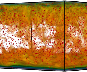
Figure 10. The temporally averaged flow field on a vertical midplane. Contours show the vertical velocity, and the streamlines are integrated with the in-plane velocity vector. Here (a)  ${\textit {St}}=0.01$, (b)
  ${\textit {St}}=0.4$, and (c)
  ${\textit {St}}=10$, respectively, and the Rayleigh number is
  ${\textit {Ra}}=10^{10}$.
Nevertheless, by using the fact that the dissipation rate is dominated by the bulk contribution, and employing the power-law scaling in figure 9(c), one obtains the following scaling relation:
 \begin{equation} {\textit{Re}}^{2.7} \sim \epsilon_u^{bulk} \frac{H^4}{\nu^3} \approx {\textit{Ra}} {\textit{Pr}}^{{-}2} \langle w\theta \rangle_V. \end{equation}
We have also shown that  $\langle w\theta \rangle _V \sim {\textit {Ra}}^{0.084}$, which implies that
 \begin{equation} {\textit{Re}} \sim {\textit{Ra}}^{0.40} {\textit{Pr}}^{{-}3/2}. \end{equation}
In figure 11 the above scaling is compared with the numerical results and the agreement is very good. Moreover, for laminar BL one has  $\lambda _u\sim {\textit {Re}}^{-1/2}\sim {\textit {Ra}}^{-0.2}$, which is also very close to the scaling of the top BL thickness in figure 3(a). For the volume-averaged temperature
  $\langle \theta \rangle _V$, we note that the total heat flux from two boundaries can be approximated as
  $\langle \theta \rangle _V / \lambda _\theta$. For laminar BLs
  $\lambda _\theta \sim \lambda _u {\textit {Pr}}^{-1/3}\sim {\textit {Re}}^{-1/2}{\textit {Pr}}^{-1/3}$. Then by using (3.3), one has
 \begin{equation} \langle \theta \rangle_{V}\sim Ra^{1/3}Pr^{1/3}\lambda_{\theta} \sim Ra^{0.133} Pr^{2/5}. \end{equation}
The exponent  $0.133$ is also close to that given by the linear fitting, see figure 5(c).

Figure 11. The compensated plot of Reynolds number  ${\textit {Re}}$ versus
  ${\textit {Ra}}$.
4. Particle distributions and different flow regimes
With the help of the flow characteristics and transport properties discussed in the previous section, the spatial distribution of particles will be investigated in this section. We first identify the boundaries of the flow regime where the consistency between simulation results and physical models holds, and then discuss the preferential concentration of particles for those cases with a statistically steady state.
4.1. Particle accumulation and different flow regimes
For some cases at  ${\textit {Ra}} \le 10^9$ and certain range of
  ${\textit {St}}$, as mentioned before and indicated by the black diamonds in figure 1, most particles will eventually accumulate into a thin layer adjacent to the top plate, where the local heating intensity is very strong. If the time step is reduced, the simulation can continue for longer time period. But eventually the time step becomes extremely small and the simulation is unfeasible. Outside this regime the flow can reach a statistically steady state in several hundreds of non-dimensional time units. The heat released from particles drives the convection flow which transport particles over the whole domain. The local particle number density remains small at all heights and the physical models we employed are still valid.
To illustrate these different states, we uniformly divide the flow domain into 40 slabs along the vertical direction. The mean number density  $c_s$ is then calculated for each slab and normalized by the initial mean number density of the entire domain. Therefore, if all particles stay in a single slab, this slab will have
  $c_s=40$. In figure 12 we plot the time history of the profile
  $c_s$ for two cases with
  ${\textit {Ra}}=10^9$ from different regimes. For the case with
  ${\textit {St}}=0.1$, at approximately 100 time units
  $c_s$ is very close to
  $40$ for the slab adjacent to the top plate, indicating that almost all particles stay within this thin layer at the top. The simulation has to stop at approximately
  $t=120$ due to the extreme large heating source close to the top boundary. Meanwhile, for the case with
  ${\textit {St}}=0.02$,
  $c_s$ is still higher at the slabs close to the top and bottom plates, but in the bulk
  $c_s$ does not approach zero. Particles can still travel inside the bulk region for this case, and finally a statistically steady state is established.

Figure 12. The time evolution of the profile of mean number density of particles for two cases with (a)  $St=0.1$ and (b)
  $St=0.02$, respectively. The Rayleigh number
  ${\textit {Ra}}=10^9$ is same for the two cases.
For some cases close to the regime where the particle accumulation happens, flow can still reach a statistically steady state and the simulation can continue. However, the normalized number density is elevated over  $10$ within the upper viscous BL adjacent to the top boundary. These cases are marked by the yellow squares in figure 1. Therefore, the transitions between these two regimes on the
  ${\textit {St}}$–
 ${\textit {Ra}}$ phase plane are not sharp ones, and can be roughly understood as follows. Two processes are responsible for the left-hand and right-hand transition boundaries in the phase space. For the first process, one can start from the large Stokes number where a statistically steady state exists. With large enough
  $St$, particles which enter the top boundary layer cannot decelerate and stop moving in the vertical direction within the top BL. As
  $St$ decreases, particles become more responsive to the change of fluid momentum. If the vertical velocity of particles can decrease to zero before particles penetrate the top BL, they will be trapped inside the BL region. For the second process, one starts from the small Stokes number where again a statistically steady state exists. Now because particles can perfectly follow the flow motions, they are carried out of the top BL by the descending plumes. However, as
  $St$ increases, particles become less responsive and they may not gain enough downward velocity to escape the top BL during the time period as they travel over the height of the top BL. In the following we establish the scaling laws for the transition boundaries based on the two processes.
For the first process, we notice that inside the viscous BL next to the top plate, the vertical velocity component  $w_f$ is small compared with the horizontal velocity component. As an approximation we take
  $w_f \approx 0$. When a particle enters the BL with a certain vertical velocity
  $w^0_p$, the vertical velocity of the particle will decrease due to the vertical component of the Stokes drag. From (2.14e) one obtains a formal solution as
 \begin{equation} w_p(t)=w_p^0\exp\left({-}t/{\textit{St}}\right). \end{equation}
Then the total height which the particle travels until  $w_p$ reaches zero is given by
 \begin{equation} \delta z_p = \int_{0}^{\infty} w_p(t) \,{\rm d}t = \int_0^{\infty}w_p^0\exp\left({-}t/{\textit{St}}\right)\,{\rm d}t=w_p^0 {\textit{St}}. \end{equation}
If  $w_p$ decreases to zero before the particle moves through the height of BL, i.e.
  $\delta z_p\le \lambda _{u,top}$, then the particle will stay within the BL. This gives a scaling relation of the minimum particle entry velocity
  $w^0_{p,min}$ for a particle to travel into and through the BL:
 \begin{equation} w_{p,min}^0 {\textit{St}} \sim \lambda_{u,top}. \end{equation}
In the previous section we have show that  $\lambda _{u,top}\sim {\textit {Re}}^{-1/2}$ and
  ${\textit {Re}}\sim {\textit {Ra}}^{2/5}$.
Meanwhile, the entry velocity  $w^0_p$ should have the same order as the velocity scale in the bulk, namely
  $w^0_p \sim U_{rms} \sim {\textit {Re}}$. When the particles are trapped in the BL by a drag force, the entry velocity
  $w^0_p$ should be smaller than
  $w^0_{p,min}$. The critical Stokes number
  ${\textit {St}}^u_{cr}$ can be obtained when
  $w^0_p \sim w^0_{p,min}$. Thus, one has
 \begin{equation} {\textit{St}}^u_{cr} \sim \lambda_u / w^0_p \sim Re^{{-}3/2} \sim Ra^{{-}3/5}. \end{equation}
Since for fixed  ${\textit {Ra}}$ and therefore fixed
  $\lambda _u$,
  $\delta z_p$ increases as
  ${\textit {St}}$ becomes larger. The first process is effective when
  ${\textit {St}}<{\textit {St}}^u_{cr}$, and particles with smaller
  ${\textit {St}}$ will stay inside the BL while those with larger
  ${\textit {St}}$ will not. This suggests that
  ${\textit {St}}^u_{cr}$ corresponds to the upper transition boundary between two regimes.
For the second process, as the particles already inside the BL cannot escape, we point out that particles escaping the top BL are mainly carried downwards by the cold plumes ejected from the top BL. The time scale for a fluid element to move through the BL can be estimated as  $\tau _f^{bl} \sim \tau _f \lambda _{u,top} / H$, in which we assume that the fluid element moves through the entire domain height
  $H$ with the time scale
  $\tau _f$. When
  $\tau _p<\tau _f^{bl}$, particles will gain a vertical downward velocity close enough to fluid velocity and are likely to be transported away from the BL. Then a scaling relation for this transition is
  $\tau _p/\tau _f^{bl} \sim 1$. Recalling that
  $\lambda _{u,top}\sim {\textit {Ra}}^{-1/5}$, one obtains
 \begin{equation} St^{l}_{cr} \sim Ra^{{-}1/5}. \end{equation}
For the second process to be effective, the Stokes number should be larger than  $St^{l}_{cr}$, and the above scaling corresponds to the lower transition boundary between the two regimes.
The two scaling relations (4.4) and (4.5) for the transition boundaries between different regimes are plotted in figure 1 with properly chosen prefactors. The above two mechanisms are both necessary for particles to accumulate in the BL, which means the Stokes number should satisfy  $St^{l}_{cr} \le {\textit {St}} \le St^{u}_{cr}$. As can be seen from figure 1, the predictions given by the above scaling analyses capture the transition boundaries every well.
4.2. Preferential concentration of particles and mean statistics
When the flow reaches the final statistically steady state, particles still exhibit preferential concentration. We first look at the vertical distribution of particles. In figure 13 we show the instantaneous flow fields and particle distributions on a vertical plane for three cases with the same  ${\textit {Ra}}=10^{10}$ and increasing
  ${\textit {St}}=0.01$,
  $0.4$ and
  $10$, respectively. For the two cases with small or large
  ${\textit {St}}$, particles are fairly uniform in the bulk. Due to the nearly uniform distribution in the bulk, the fluid temperature is also relatively high as particles are heating the fluid. However, for the case with intermediate
  ${\textit {St}}$, particles show clear non-uniform distribution. The number density is higher near the top and bottom boundaries, and inside the rising flow in the bulk, as can be seen by comparing figure 13(b) and figure 13(e).

Figure 13. (a–c) The contours of vertical velocity on a middle vertical plane, and (d–f) the contours of temperature field along with the instantaneous particle distribution on the same vertical plane, respectively. Here (a,d), (b,e) and (c,f) are  ${\textit {St}}=0.01$,
  $0.4$ and
  $10$, respectively. The Rayleigh number is
  ${\textit {Ra}}=10^{10}$.
To quantitatively measure the possible non-uniform distribution along the vertical direction, figure 14(a) plots the probability density function (p.d.f.) of the vertical location  $z$ of particles for the five cases with fixed
  ${\textit {Ra}}=10^{10}$ and different
  ${\textit {St}}$. For the largest
  ${\textit {St}}=10$ and the smallest
  ${\textit {St}}=0.01$, the p.d.f. is lower near the bottom boundary, and higher near the top boundary. The difference is that for
  ${\textit {St}}=0.01$, the p.d.f. has a single peak close to the top boundary. While for
  ${\textit {St}}=10$, the high p.d.f. happens in a wider region without an apparent peak near the top. For the three intermediate Stokes numbers, their p.d.f.s all have two peaks located close to the top and bottom plates, and are relatively low in the bulk, indicating stronger non-uniformity along the vertical direction. The fact that p.d.f. is the lowest in the bulk for
  ${\textit {St}}=0.1$ and
  $0.4$ is consistent with the behaviours shown in figure 5. Since particles release heat to the surrounding fluid, lower number density in the bulk corresponds to weaker heating source and volume-averaged temperature is also smaller.

Figure 14. (a) The probability density function of the vertical positions of particles. (b) The Stokes number  ${\textit {St}}_\eta$ defined by the local Kolmogorov time scale versus the height. For all the shown cases
  ${\textit {Ra}}=10^{10}$.
The different shapes of p.d.f.s for different  ${\textit {St}}$ can be understood as follows. In figure 14(b) we plot the vertical profiles of
  ${\textit {St}}_\eta =\tau _p/\tau _\eta$ with
  $\tau _\eta = \eta _u^2/\nu$ being the local Kolmogorov time scale. Here
  $\eta _u$ is the Kolmogorov length scale calculated at each height. Here
  ${\textit {St}}_\eta$ is slightly larger than
  ${\textit {St}}$ in all cases. Still, for
  ${\textit {St}}=0.01$ and
  $10$,
$10$,  ${\textit {St}}_\eta$ is far away from unit and the momentum coupling between flow and particles is weak. When
  ${\textit {St}}=0.01$ the particles follow the fluid almost perfectly. Since particles release heat into the surrounding fluid, particles are more likely to rise towards the top plate, and stay at the top until being carried away by the downward plumes. For
  ${\textit {St}}=10$, the particle inertia is very large and their movement is hardly affected by the flow. They prefer to move upward due to the heat-releasing effect. But when they move towards the top plate, they can easily penetrate the BL, rebound at the top boundary, and then leave the top BL due to the large inertia. Therefore, p.d.f. does not have a peak near the top plate as in the case with
  ${\textit {St}}=0.01$. For the other three cases,
  ${\textit {St}}_\eta$ is close to unity and the momentum coupling is strong between the fluid flow and the particles. It is well known that the preferential concentration is most distinct for
  ${\textit {St}}_\eta \approx 1$ in turbulent channel flows (Sardina et al. Reference Sardina, Schlatter, Brandt, Picano and Casciola2012). Also as discussed in the previous section, for the cases with intermediate
  ${\textit {St}}$, particles are more likely to be trapped within the BL regions where the vertical velocity is small.
The preferential concentration in the horizontal directions is examined by the Voronoï diagrams (Ferenc & Néda Reference Ferenc and Néda2007; Monchaux, Bourgoin & Cartellier Reference Monchaux, Bourgoin and Cartellier2010; Yang et al. Reference Yang, Zhang, Wang, Dong and Zhou2021). That is, the horizontal plane is divided into Voronoï cells based on particle locations. The area  $A$ of the Voronoï cell associated with each particle is inversely correlated to the local concentration of particles. We choose three horizontal planes at the edges of two viscous BLs and
  $z/H=0.5$. Typical Voronoï diagrams on these planes are shown in figure 15 for three cases with fixed
  ${\textit {Ra}}=10^{10}$ and
  ${\textit {St}}=0.01$,
  $0.4$ and
  $10$, respectively. For
  ${\textit {St}}=0.4$, the preferential concentration is strongly presented in all three heights. Small clusters form large clusters which non-uniformly distribute over the horizontal planes. For
  ${\textit {St}}=10$, small clusters can be observed but they do not form large clusters, but randomly distribute over the plane. For
  ${\textit {St}}=0.01$, the behaviours are similar to those with
  ${\textit {St}}=10$ at the mid plane and the edge of top viscous BL. However, large voids with nearly no particles form at the edge of bottom viscous BL. This is because particles with
  ${\textit {St}}=0.01$ are more likely to be carried away from the bottom viscous BL by fluid motions.

Figure 15. Typical snapshots of the horizontal distribution of particles and their Voronoï diagram for  $Ra=10^{10}$ and different
  ${\textit {St}}$: (a–c)
  ${\textit {St}}=0.01$; (d–f)
  ${\textit {St}}=0.4$; (g–h)
  ${\textit {St}}=10$. Here (a,d,g), (b,e,h) and (c,f,i) are
  $z=\lambda _{u,bot}, 0.5H, H-\lambda _{u,top}$, respectively.
The p.d.f.s of the area of Voronoï cells are sampled at three different heights and plotted in figure 16 for different Stokes numbers and fixed  ${\textit {Ra}}=10^{10}$. The p.d.f. for a random Poisson process (RPP), which corresponds to the uniformly random distribution of particles, is shown for comparison. For all three heights, the right-hand tails of the p.d.f.s approach the RPP distribution as
  ${\textit {St}}$ becomes larger, while a flat tail always exists on the left-hand side. Moreover, the left-hand tails exhibit different behaviours at different heights as
  ${\textit {St}}$ increases. For both the midheight and the edge of the top BL, p.d.f. at small
  $A/\langle A \rangle _p$ is highest at the intermediate Stokes numbers, indicating the strongest preferential concentration due to the momentum interaction between fluid and particles. At the edge of the bottom BL, the p.d.f. of the smallest
  ${\textit {St}}=0.01$ has the highest left-hand tail, consistent with the distribution shown in figure 15(a–c).

Figure 16. The p.d.f.s of normalized Voronoï area  $A/\langle A \rangle _p$ in the horizontal planes for different
  ${\textit {St}}$ and
  ${\textit {Ra}}=10^{10}$: (a)
  $z=\lambda _{u,bot}$; (b)
  $z=0.5H$; (c)
  $z=H-\lambda _{u,top}$.
Figure 17 displays the p.d.f.s of the area of Voronoï cells for two fixed  ${\textit {St}}$ and increasing
  ${\textit {Ra}}$ at three heights. For
  ${\textit {St}}=0.01$, the clustering at the edge of the bottom BL becomes stronger as
  ${\textit {Ra}}$ increases, as indicated by the elevation of the left-hand tails in figure 17(a). Meanwhile, the right-hand tails deviate from the RPP distribution. At the midheight and the edge of top BL, the influence of increasing
  ${\textit {Ra}}$ is much smaller. For
  ${\textit {St}}=10$, the p.d.f. does not change much with
  ${\textit {Ra}}$ at all three heights. The right-hand tails are very close to the RPP distribution, and the flat left-hand tails are produced by the small clusters shown in figure 15.

Figure 17. The p.d.f.s of normalized Voronoï area  $A/\langle A \rangle _p$ in the horizontal planes for different
  ${\textit {St}}$ and
  ${\textit {Ra}}$: (a,d)
  $z=\lambda _{u,bot}$; (b,e)
  $z=0.5H$; (c,f)
  $z=H-\lambda _{u,top}$. Here panels (a–c) are for
  ${\textit {St}}=0.01$, and (d–f) for
  ${\textit {St}}=10$, respectively.
To quantitatively investigate the multiscale nature of particle clusters on horizontal planes, we employ the radial distribution functions (RDF) (e.g. Ireland, Bragg & Collins Reference Ireland, Bragg and Collins2016). The RDF  $g(r)$ is calculated by
 \begin{equation} g(r)=\frac{N_r/V_r}{N/V}. \end{equation}
Here,  $N_i$ is the number of particle pairs whose separation distances fall inside the shell with a radius range
  $(r-\Delta r/2, r+\Delta r/2)$. Here
  $V_r$ is the volume of the corresponding shell in the distance space,
  $N$ is the total number of particle pairs and
  $V$ is the total volume. When
  $g(r)$ is equal to
  $1$, the particle field is uniformly distributed. Here
  $g(r)$ greater than unity indicates a clustered particle field at scale
  $r$.
$r$.
The 2-D RDFs are computed over the horizontal slices at  $z=\lambda _{u,bot}$,
  $z=0.5H$ and
  $z=H-\lambda _{u,top}$ for fixed
  ${\textit {Ra}}=10^{10}$ and different
  ${\textit {St}}$, which are shown in figure 18. At the lower slice shown,
  $g(r)$ is considerably larger than
  $1$ for almost all the computed distance
  $r$ at
  ${\textit {St}}=0.01$, corresponding to the large voids shown in figure 15(a). As
  ${\textit {St}}$ increases,
  $g(r)$ gradually decreases at nearly all
  $r$. This is consistent with figure 15(a,d,g), where large voids at
  ${\textit {St}}=0.01$ transit into large clusters at
  ${\textit {St}}=0.4$ and then nearly uniformly distributed small clusters at
  ${\textit {St}}=10$. At the two higher slices with
  $z=0.5H$ and
  $H-\lambda _{u,top}$,
  $g(r)$ experiences non-monotonic variations as
  ${\textit {St}}$ becomes larger. Now
  $g(r)$ exceeds unity over wider range of
  $r$ for intermediate
  ${\textit {St}}$, indicating again the preferential distribution with large clusters formed by small clusters.

Figure 18. The RDFs in the horizontal planes for different  ${\textit {St}}$ and fixed
  ${\textit {Ra}}=10^{10}$: (a)
  $z=\lambda _{u,bot}$; (b)
  $z=0.5H$; (c)
  $z=H-\lambda _{u,top}$.
5. Conclusions
In this work we conducted a systematic study of the convection flow driven by heat-releasing point particles which absorb energy from an external source. The energy absorbed by particles is then released to heat the surrounding fluid, which drives the buoyancy flow motions in the domain. The heat is then transferred out from the domain through the top and bottom plates. We confine ourselves within the parameter space where the global volume fraction of particles is small and the Froude number is large, so that one-way coupling is used for momentum interaction and two-way coupling for thermal interaction, respectively. Meanwhile, the gravitational settling of particles is neglected. The current study then focuses on the influences of the Rayleigh number  ${\textit {Ra}}$ within the range
  $(10^7,10^{10})$ and the Stokes number
  ${\textit {St}}$ within the range
  $(0.01,10)$, while the other non-dimensional numbers are fixed.
Within the parameter range simulated here, we reveal a regime in which nearly all the particles will eventually accumulate towards the top plate. We identify the physical mechanism of this accumulation as the interaction between the inertial particles and the top BL. Specifically, for intermediate Stokes numbers at certain Rayleigh number, the particles do not respond to the fluid motion quickly enough and cannot be carried away from the BL. Meanwhile, their inertia is not too strong to fully decouple with the flow within the BL. By scaling analyses we propose the upper and lower boundaries in the  ${\textit {Ra}}-{\textit {St}}$ phase plane, which can describe the numerical results perfectly. Outside this regime, the flow can reach a statistically steady state with particles constantly advected over the entire domain.
For the flow at a statistically steady state, the flow and mean statistics are asymmetric between the upper and lower parts of the domain. The flow motions are stronger in the upper part of bulk region, and the top BL is thinner than the bottom one for both momentum and temperature fields. Both the volume-averaged temperature and convective heat flux exhibit non-monotonic dependences on  ${\textit {St}}$ and their minima are expected to locate at
  $0.1\le {\textit {St}}\le 0.4$. The fraction coefficient
  $F_B$, which measures the asymmetry between the heat fluxes through the top and bottom plates, is dominated by the convective flux. Our numerical results indicate that the dependences of both the convective flux and
  $F_B$ on
  ${\textit {Ra}}$ are similar to those reported for internally heated RB with a uniform source.
However, our investigations also reveal several behaviours which are different from the internally heated RB with a uniform source. The viscous dissipation rate is dominated by the contribution from the bulk, while for uniformly heated RB with similar driving strength, the dominant contribution comes from the BLs. Also, in the current flow large-scale convection rolls develop in the bulk which were not found in the 3-D simulations of uniformly heated RB (Goluskin & van der Poel Reference Goluskin and van der Poel2016). Nevertheless, by using the global balance between the dissipation rate and the convective flux and by adopting the relation extracted from the numerical data, the scaling behaviours of the Reynolds number, the volume-averaged temperature and the thicknesses of BLs can be explained.
Preferential concentration is also observed in the present flow. For intermediate Stokes numbers, particles have higher number density in both the top and bottom viscous BLs. In the horizontal directions the clustering of particles has a multiscale nature: the horizontal RDFs exceed unity over a wide range of particle separation distance at planes with different height. For small and large Stokes numbers, the multiscale clustering in the horizontal directions is much weaker. It should be pointed out, though, for the smallest Stokes number large voids with very low particle number density were observed over the horizontal plane near the bottom plate. Since the local strength of heating source strongly depends on the local particle concentration, the preferential concentration should have profound influences on the convection motions. This may explain the differences between the present flow and the uniformly heated RB.
The current work opens up several interesting directions for future study. For instance, two-way coupling in the momentum interaction can be included and the gravitational settling of particles may be considered. Note that gravitational settling and the heat-releasing to the surrounding fluid have competing effects on the vertical translation of particles, and non-trivial behaviours can be expected when the gravitational settling process is introduced in the system. These are the subjects of our ongoing research.
Fundings
This work is financially supported by the Marine S&T Fund of Shandong Province for Pilot National Laboratory for Marine Science and Technology (Qingdao) (no. 2022QNLM010201) and the Major Research Plan of National Natural Science Foundation of China for Turbulent Structures under the grants 91852107.
Declaration of interests
The authors report no conflict of interest.
Appendix A. Numerical details
Table 1. Summary of the numerical simulations. Columns from left to right are the Rayleigh number, the Stokes number, the resolutions in the horizontal and vertical directions, the fraction of internally heat across bottom boundaries, the Reynolds number based on the r.m.s. value of velocity, the mean system temperature, the thickness of top and bottom viscous BL, the thickness of temperature BL, the mean concentration  $c_s$ for the top BL, the mean temperature difference of two phases, the non-dimensional total heat flux across top and bottom plates
  $Nu$, respectively. The resolution in the
  $y$ direction is the same as that in the
  $x$ direction. For all cases the aspect ratio of the domain
  $L=4$, the Prandtl number
  $Pr=0.7$, the non-dimensional particle number density
  $C=1\times 10^5$, the heat-capacity ratio
  $\varPhi _{\theta }=0.1$ and the heat-mixing parameter
  $\sigma =1$.


