


1. Introduction
Symmetry breaking exists widely in the fluid world. One typical symmetry is the axial symmetry, which is normally associated with axisymmetric bodies such as circular disks or spheres. Complicated axial symmetry breaking phenomena occur in the wake behind the fixed circular disk (see e.g. Marshall & Stanton Reference Marshall and Stanton1931; Michael Reference Michael1966; Kuo & Baldwin Reference Kuo and Baldwin1967; Rimon Reference Rimon1969; Roos & Willmarth Reference Roos and Willmarth1971; Roberts Reference Roberts1973; Rivet et al. Reference Rivet, Henon, Frisch and d'Humieres1988; Berger, Scholz & Schumm Reference Berger, Scholz and Schumm1990; Natarajan & Acrivos Reference Natarajan and Acrivos1993; Fernandes et al. Reference Fernandes, Risso, Ern and Magnaudet2007; Fabre, Auguste & Magnaudet Reference Fabre, Auguste and Magnaudet2008; Shenoy & Kleinstreuer Reference Shenoy and Kleinstreuer2008, Reference Shenoy and Kleinstreuer2010; Meliga, Chomaz & Sipp Reference Meliga, Chomaz and Sipp2009; Auguste, Fabre & Magnaudet Reference Auguste, Fabre and Magnaudet2010; Chrust, Bouchet & Dušek Reference Chrust, Bouchet and Dušek2010; Yang et al. Reference Yang, Liu, Wu, Zhong and Zhang2014, Reference Yang, Liu, Wu, Liu and Zhang2015) and sphere (see e.g. Barkla & Auchterlonie Reference Barkla and Auchterlonie1971; Sakamoto & Haniu Reference Sakamoto and Haniu1990; Johnson & Patel Reference Johnson and Patel1999; Fabre et al. Reference Fabre, Auguste and Magnaudet2008; Chrust, Goujon-Durand & Wesfreid Reference Chrust, Goujon-Durand and Wesfreid2013). It is known that these wake transition processes involve several stages that have general similarities, but with some differences between the disk and sphere wakes.
The transition scenarios of the circular disk are determined by both the disk aspect ratio and the free stream Reynolds number. Here, the aspect ratio of the circular disk is defined as  $\chi =D/t_d$, where
  $D$ is the disk diameter and
  $t_d$ is the disk thickness. The free stream Reynolds number is defined as
  $Re_s=U_\infty D/\nu$, where
  $U_\infty$ is the free stream velocity, and
  $\nu$ is the kinematic viscosity of the fluid. In what follows, the aspect ratio
  $\chi =\infty$ is considered a ‘flat disk’ or an infinitely thin disk. For a very low Reynolds number, the steady and axisymmetric flow is described by Shenoy & Kleinstreuer (Reference Shenoy and Kleinstreuer2008) and is called the ‘trivial’ state by Auguste et al. (Reference Auguste, Fabre and Magnaudet2010). The first bifurcation occurs at the critical Reynolds number
  ${Re_s^{c1}}$, namely,
  ${Re_s^{c1}}=135$ in Shenoy & Kleinstreuer (Reference Shenoy and Kleinstreuer2008) (
 $\chi =10$),
  ${Re_s^{c1}}=129.6$ in Chrust et al. (Reference Chrust, Bouchet and Dušek2010) (
 $\chi =10$),
  ${Re_s^{c1}}=159.4$ in Auguste et al. (Reference Auguste, Fabre and Magnaudet2010) (
 $\chi =3$), and
  ${Re_s^{c1}}=115\unicode{x2013}117$ according to Natarajan & Acrivos (Reference Natarajan and Acrivos1993), Fabre et al. (Reference Fabre, Auguste and Magnaudet2008), Meliga et al. (Reference Meliga, Chomaz and Sipp2009) and Chrust et al. (Reference Chrust, Bouchet and Dušek2010) (
 $\chi =\infty$). Moreover, the threshold is related to the aspect ratio, and the formula given by Fernandes et al. (Reference Fernandes, Risso, Ern and Magnaudet2007) is
  $Re_s^{c1} \approx 116.5(1+\chi ^{-1})$. Subsequently, the wake is featured by a steady non-axisymmetric but reflectional symmetric state, which gives rise to a steady lift force in the symmetric plane and a pair of steady streamwise vortices. This state is named after both the ‘steady state’ (Fabre et al. Reference Fabre, Auguste and Magnaudet2008; Meliga et al. Reference Meliga, Chomaz and Sipp2009) and the ‘steady asymmetric state’ (Shenoy & Kleinstreuer Reference Shenoy and Kleinstreuer2008). The characteristics of these two stages are similar to the case of a sphere except that the value of
  ${Re_s^{c1}}$ is found to be 212 for a sphere (Johnson & Patel Reference Johnson and Patel1999).
The second Hopf bifurcation is observed for the critical Reynolds number  $Re_s^{c2} = 136.3\unicode{x2013}138.7$ by Chrust et al. (Reference Chrust, Bouchet and Dušek2010) (
 $\chi = 10$) and
  $Re_s^{c2} \approx 155$ by Shenoy & Kleinstreuer (Reference Shenoy and Kleinstreuer2008) (
 $\chi = 10$). For a flat disk with
  $\chi = \infty$, it is widely accepted that the range of
  ${Re_s^{c2}}$ is between 121 and 125.6, as reported by Natarajan & Acrivos (Reference Natarajan and Acrivos1993), Fabre et al. (Reference Fabre, Auguste and Magnaudet2008), Meliga et al. (Reference Meliga, Chomaz and Sipp2009) and Chrust et al. (Reference Chrust, Bouchet and Dušek2010). Fernandes et al. (Reference Fernandes, Risso, Ern and Magnaudet2007) summarize the relation between
  $Re_s^{c2}$ and
  $\chi$ as
  $Re_s^{c2} \approx 125.6(1+\chi ^{-1})$. The disk experiences the oscillating lift force about a mean value; meanwhile, the oscillation is perpendicular to the symmetry plane determined by the first bifurcation. This state is denoted as ‘reflectional symmetry breaking’ (RSB) by Fabre et al. (Reference Fabre, Auguste and Magnaudet2008), ‘three-dimensional periodic flow with regular rotation of the separation region’ by Shenoy & Kleinstreuer (Reference Shenoy and Kleinstreuer2008), ‘mixed mode with phase
  ${\rm \pi}$’ (
 ${\rm MM}_{\rm \pi}$) by Meliga et al. (Reference Meliga, Chomaz and Sipp2009), or the ‘yin-yang’ mode by Auguste et al. (Reference Auguste, Fabre and Magnaudet2010). Specifically, for the thick disk with
  $\chi =3$ studied by Auguste et al. (Reference Auguste, Fabre and Magnaudet2010), the flow undergoes ‘zig-zig’, ‘knit-knot’ and ‘yin-yang’ modes successively after the Hopf bifurcation. Here, the ‘knit-knot’ mode refers to the reflectional symmetric state with a lift force oscillating around a non-zero mean value. Although this mode is different from that of the disk above, the feature is identical to a ‘reflectional symmetry preserving’ mode (Fabre et al. Reference Fabre, Auguste and Magnaudet2008) in a sphere wake.
The next bifurcation has been found at  $Re_s^{c3} \approx 140\unicode{x2013}143$ by Fabre et al. (Reference Fabre, Auguste and Magnaudet2008), Meliga et al. (Reference Meliga, Chomaz and Sipp2009) and Chrust et al. (Reference Chrust, Bouchet and Dušek2010), successively, for an infinitely thin disk. This state can be distinguished from the RSB mode on account of the recovery of the reflectional symmetry plane. As a consequence, the state is called ‘unsteady with planar symmetry and zero lift force’ (Shenoy & Kleinstreuer Reference Shenoy and Kleinstreuer2008), ‘standing wave’ (SW) (Fabre et al. Reference Fabre, Auguste and Magnaudet2008; Meliga et al. Reference Meliga, Chomaz and Sipp2009) and ‘zig-zag’ mode (Auguste et al. Reference Auguste, Fabre and Magnaudet2010). As the Reynolds number increases further, the flow develops from a quasi-periodic state to a chaotic state. In the quasi-periodic state, a secondary frequency close to one-third of the primary frequency of the previous regimes appears (Auguste et al. Reference Auguste, Fabre and Magnaudet2010), and the modulation is also evidenced in the sphere wake (Bouchet, Mebarek & Dušek Reference Bouchet, Mebarek and Dušek2006). In addition, Chrust et al. (Reference Chrust, Bouchet and Dušek2010) summarized a systematic
  $Re_s\unicode{x2013}\chi$ parametric map for oblate spheroids and disks with
  $\chi \geqslant 1$.
It is noted that the breaking of axisymmetric flow is influenced not only by  $Re_s$ but also by the rotational motion of the body. It is worth noting that in most cases, the effect of rotational motion on symmetry breaking is even more evident. For example, the trajectory of the rotating ball is curved. The flow around a rotating body depends significantly on the direction of rotation, which may be either parallel or perpendicular to the free stream direction, namely, streamwise rotation and transverse rotation, respectively. In this paper, we focus on streamwise rotation, on which numerous studies have been conducted in recent years for the sphere (see e.g. Kim & Choi Reference Kim and Choi2002; Pier Reference Pier2013; Poon et al. Reference Poon, Ooi, Giacobello and Cohen2010; Neeraj & Tiwari Reference Neeraj and Tiwari2018; Skarysz et al. Reference Skarysz, Rokicki, Goujon-Durand and Wesfreid2018; Lorite-Díez & Jiménez-González Reference Lorite-Díez and Jiménez-González2020).
The rotational motion of the body is represented using a non-dimensional rotation rate  $\varOmega$, where
  $\varOmega$ is the maximum azimuthal velocity on the rotating sphere normalized by the free stream velocity. As the Reynolds number is low enough, the flow is in a steady and axisymmetric state. This state has been called ‘steady axisymmetric’ flow (Kim & Choi Reference Kim and Choi2002) and ‘the axisymmetric steady base flow (either stable or unstable)’ regime (Pier Reference Pier2013). A reasonable consensus has been reached that the unsteady wake is the periodic regime with no temporal variation in either the shape of the vortical structure or the spin around the axis. This mode is observed as ‘frozen’ by Kim & Choi (Reference Kim and Choi2002) and Neeraj & Tiwari (Reference Neeraj and Tiwari2018), ‘the low-frequency periodic helical’ regime by Pier (Reference Pier2013), and the ‘low-helical’ regime by Skarysz et al. (Reference Skarysz, Rokicki, Goujon-Durand and Wesfreid2018). With a higher value of the streamwise Reynolds number
  $Re_s$, the frozen rotation of the vortical structure in combination with variations in its shape indicates the quasi-periodic vortex shedding regime (Pier Reference Pier2013) and the unsteady asymmetry regime (Kim & Choi Reference Kim and Choi2002). The transition between the quasi-periodic and chaotic regimes is similar to frozen rotation, but it rotates at a higher frequency, which is referred to as ‘frozen’ by Kim & Choi (Reference Kim and Choi2002) at
  ${Re}=300$ and ‘the high-frequency periodic helical’ regime by Pier (Reference Pier2013). As a consequence, Lorite-Díez & Jiménez-González (Reference Lorite-Díez and Jiménez-González2020) concluded a summary (
 $\varOmega, Re_s$) map about the flow regimes for a streamwise rotating sphere. Moreover, the modification of the axis of rotation and non-dimensional rotation rate have a significant effect on the state of the wake structures, as Poon et al. (Reference Poon, Ooi, Giacobello and Cohen2010) demonstrated.
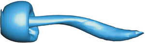
Earlier studies of the flow around a streamwise rotating sphere successfully confirmed these complicated transition scenarios. However, similar studies have not been reported for circular disks. It is notable that the main difference between the disk and sphere is that the disk is a sharp-edged body, while the sphere is more streamlined. Based on the conclusion of the wake transition of a fixed disk and sphere, the transition process of the circular disk is more complicated, and the critical Reynolds number is lower than that of the sphere. It is expected that there are some new and interesting phenomena in the wake of a rotating disk, and several questions arise. (i) What is the wake behind the streamwise rotating circular disk? (ii) How many flow states exist, and what is the threshold between them? (iii) How does the streamwise rotation affect the wake and threshold of the circular disk? (iv) What is the similarity or difference between a streamwise rotating disk and a streamwise rotating sphere? To answer these questions, we consider a simple condition that the uniform flow is normal to a streamwise rotating disk, as shown in figure 1.

Figure 1. Sketch of the uniform flow past a streamwise rotating circular disk. The origin of the coordinate system is in the geometric centre of the disk as defined. The  $x$ axis is the free flow direction, which corresponds to the direction of rotation of the disk.
Following the non-dimensional rotation rate  $\varOmega$ defined for the rotating sphere (Kim & Choi Reference Kim and Choi2002), a new Reynolds number describing the rotational motion is defined as
  $Re_r=\varOmega Re_s$, where the non-dimensional rotation rate of the disk,
  $\varOmega =\frac {1}{2}\omega D/U_\infty$, is based on the angular rotation speed of the disk,
  $\omega$. Chrust et al. (Reference Chrust, Bouchet and Dušek2010) demonstrated that the flat cylinder (
 $\chi \geqslant 4$) and the infinitely thin disk have similar transition processes. In that way, a circular disk with aspect ratio 50 can be considered a sufficiently thin disk. In addition, the ranges of the two key dimensionless parameters considered in this paper are
  $50\leqslant Re_s\leqslant 250$ and
  $0 \leqslant Re_r \leqslant 250$, respectively. On the one hand, in the scope of
  ${Re_s}$, the circular disk without rotation can completely experience all states from stable to chaotic. On the other hand, the results of preliminary calculations show several major bifurcations of flow around the circular disk when
  ${Re_r}=250$. Within this
  ${Re_s}\unicode{x2013}{Re_r}$ region, direct numerical simulations are used in this study to obtain all the information of the flow field.
The remainder of this paper is structured as follows. The numerical methods and studies of mesh convergence and code validation are presented in § 2. The results and discussions are offered in § 3. Finally, the concluding remarks are outlined in § 4.
2. Numerical simulations
2.1. Mathematical formulations and numerical methods
We consider a rotating circular disk subjected to a Newtonian incompressible fluid. The flow is governed by the Navier–Stokes equations, which are solved here in the Cartesian coordinate system ( $x, y, z$). These coordinates can be denoted uniformly as
  $x_i$, where
  $i=1, 2, 3$, and
  $u_i$ is the velocity component of the corresponding direction. The Navier–Stokes equations are expressed as
 $$\begin{gather} \frac{\partial u_i}{\partial x_i}=0, \end{gather}$$
 $$\begin{gather}\frac{\partial u_i}{\partial t}+u_j\,\frac{\partial u_i}{\partial x_j} ={-}\frac{1}{\rho}\,\frac{\partial p}{\partial x_i}+\nu\,\frac{\partial^2 u_i}{\partial x_j\, \partial x_j} , \end{gather}$$
where  $j=1,2,3$, and
  $p$ and
  $\rho$ are the pressure and density of the fluid, respectively. For clarity, the velocity components
  $u_1$,
  $u_2$ and
  $u_3$ are also denoted by
  $u_x$,
  $u_y$ and
  $u_z$, respectively.
These equations were discretized using the finite volume method based on the open source computational fluid dynamics code OpenFOAM, which is an object-oriented code that enables the operation and manipulation of tensor data to solve continuum mechanics problems in Weller et al. (Reference Weller, Tabor, Jasak and Fureby1998). The pimpleFoam solver is employed in the discrete governing equations, which is a transient solver for studying the incompressible turbulence of Newtonian fluids on a moving grid using the PIMPLE algorithm. The discretization of each term was undertaken by integrating the term over a control volume using Gauss's theorem, followed by linearization of volume and surface integrals using suitable schemes. The spatial schemes of interpolation, gradient, Laplacian and divergence were all linear and of second order. An additional correction was performed for the Laplacian term by interpolating cell centre gradients. The second-order Crank–Nicolson scheme was introduced for the time integration. Further detailed information about these schemes was presented previously (OpenFOAM 2021).
A spherical computational domain is adopted here, as shown in figure 2. The origin of the three-dimensional Cartesian coordinate system is located at the centre of the circular disk, which is also the centre of the computational domain. The positive direction of the  $x$ axis is the free stream direction, which is also the rotation direction of the disk. The force acting on a disk can be decomposed into three components,
  ${F_x}$,
  ${F_y}$ and
  ${F_z}$, along the coordinate system directions, which can be calculated by integrating the pressure and viscous shear stress on the disk surface. Then the force coefficients in each direction are non-dimensionalized as follows:
 \begin{equation} (C_x,C_y,C_z)=\frac{(F_x,F_y,F_z)}{\frac{1}{8}\rho U_{\infty}^2{\rm \pi} D^2}. \end{equation}
Figure 2. Schematic representation of the computational grid. (a) Overall view of the spherical computational domain and boundaries. (b) View of the grids near the disk surface.
Since the  $x$ direction is the streamwise direction,
  ${C_x}$ represents the drag coefficient, and
  ${C_y}$ and
  ${C_z}$ represent the components of the lift coefficient
  ${C_l}$ in the
  $y$ and
  $z$ directions, respectively. The magnitude of the total lift coefficient is calculated as
 \begin{equation} C_l = \sqrt{C_y^2+C_z^2}. \end{equation}
 The pressure coefficient is calculated using the reference pressure  $p_\infty$ at the centre of the inlet boundary:
 \begin{equation} C_p=\frac{p-p_\infty}{\frac{1}{2}\rho U_{\infty}^2}. \end{equation}
 The vorticity components in the  $x$ and
  $z$ directions can be expressed as
 $$\begin{gather} \omega_x = \frac{\partial u_z}{\partial y}-\frac{\partial u_y}{\partial z}, \end{gather}$$
 $$\begin{gather}\omega_z = \frac{\partial u_y}{\partial x}-\frac{\partial u_x}{\partial y}. \end{gather}$$
 The three-dimensional vortical structures are identified by the  $Q$-criterion proposed by Hunt, Wray & Moin (Reference Hunt, Wray and Moin1988), using the strain tensor
  $\boldsymbol{\mathsf{S}}$ and the rotation tensor
  $\boldsymbol {\varOmega }$:
 \begin{equation} Q ={-}\tfrac{1}{2}(\| \boldsymbol{\mathsf{S}} \| ^2-\| \boldsymbol{\varOmega} \| ^2). \end{equation}
 As shown in figure 2(a), at the inlet boundary, a uniform flow  ${U_\infty }$ is prescribed for velocity, and the pressure condition is set as a zero normal gradient. At the outlet boundary, the velocity is given as a zero normal gradient condition, and the pressure is set to zero. At the disk surfaces, the pressure is set as a zero normal gradient, and the velocity is set as the moving wall condition, where the flux is corrected in motion to ensure that the flux of the moving wall is zero. A hexahedral mesh was used for the whole computing domain, and the mesh was successfully applied and verified by Tian et al. (Reference Tian, Xiao, Zhang, Yang, Tao and Yang2017) and Gao et al. (Reference Gao, Tao, Tian and Yang2018). The grid near the disk surface is of finer resolution to resolve the steep gradient there; see figure 2(b).
To realize rotational motion of the disk around the  $x$ axis, the moving wall condition is used in the disk surfaces, where the rotating velocity on the disk surfaces is achieved by rotating the mesh points. Based on the initial permanent static mesh, as shown in figure 2(a), the mesh rotates as a whole rigid body, in which the mesh points are updated at each time step by moving the points of the mesh in the corresponding
  $yz$ plane. Let
  $\boldsymbol {X}(i,t)$ represent the spatial coordinates of point
  $i$ at time
  $t$. Since the
  $x$ axis is the rotation axis, the
  $x$ value of each coordinate point remains unchanged, while the
  $y$ and
  $z$ values rotate and transform with time. The rotation matrix
  $\boldsymbol{\mathsf{R}}$ can be used to complete the rotation transformation on the spatial coordinates, and the matrix is as follows:
 \begin{equation} \boldsymbol{\mathsf{R}} = \left[
\begin{array}{@{}ccc@{}} 1 & 0 & 0 \\ 0 &
\cos(\omega t) &
-\sin(\omega t) \\ 0 &
\sin(\omega t) & \cos(\omega
t ) \end{array} \right],
\end{equation}
\begin{equation} \boldsymbol{\mathsf{R}} = \left[
\begin{array}{@{}ccc@{}} 1 & 0 & 0 \\ 0 &
\cos(\omega t) &
-\sin(\omega t) \\ 0 &
\sin(\omega t) & \cos(\omega
t ) \end{array} \right],
\end{equation}
where  $\omega$ is the angular rotation speed of the disk. Then
  $\boldsymbol {X}(i,t)$ can be found by the following formula:
 \begin{equation} \boldsymbol{X}(i,t)=\boldsymbol{\mathsf{R}}\,\boldsymbol{X}(i,0). \end{equation}
2.2. Convergence studies
The effect of spatial and temporal resolutions on numerical simulations was evaluated by convergence analysis, and the appropriate mesh size was selected accordingly. In this sense, five numerical simulation settings with different combinations of grid elements, time steps and computational domain sizes were selected, namely, cases A, B, C, D and E, as shown in table 1. For each case, four groups of different flow configurations were calculated, and the mean values of the force coefficients  ${C_x}$ and
  ${C_l}$ are exhibited in table 2. The flow configurations include the boundary values of the considered space
  $({Re_s}, {Re_r}) = (50,200)$,
  $(200,50)$,
  $(250,250)$, and the middle of the map,
  $(150,100)$.
Table 1. Set of five cases with different spatial and temporal resolutions, where  $n_1/D$ defines the dimensionless size of the smallest cells near the disk surface,
  $\Delta t U_\infty /D$ defines the dimensionless time step, and
  $R_d$ is the radius of the spherical computational domain.

Table 2. Statistical results of force coefficients  $C_x$ and
  $C_l$ obtained from cases of four flow configurations (
 $Re_s,Re_r$). The notation
  $\langle \cdot \rangle$ denotes the mean value.

As shown in table 1, the number of grid elements of the first four cases (A, B, C and D) increases successively, and correspondingly, their non-dimensional time steps  $\Delta t\,U_\infty /D$ and smallest cell sizes
  $n_1$ decrease. As seen from the mean value of the force coefficients in table 2, the corresponding statistical results of the force coefficients
  ${C_x}$ and
  ${C_l}$ of each case have good consistency. For the cases at large Reynolds numbers, the flow becomes turbulent and a small variation around
  ${\pm }1\,\%$ exists in the mean drag coefficient between different cases. Therefore, it is concluded that the number of grid elements and the time step used in case C have acceptable accuracy. In addition, the influence of the size of the computational domain
  ${R_d}$ on the numerical simulation can be acquired by comparing cases C and E. The mesh structure and topology of case E are exactly the same as those of grid C, but the radius of the spherical computational domain
  $R_d$ is reduced from
  $30D$ to
  $20D$. The numerical results are in good agreement with those of case C, indicating that the spherical computational domain with radius
  $20D$ is large enough that the influence of the external boundary can be neglected. As shown in figure 3, for all four flow configurations, the distribution of
  $\langle C_p \rangle$ along the centreline
  $y=z=0$ of the streamwise rotating disk shows good consistency between the five different meshes. Thus for all the numerical simulations reported in the next section, the configurations of case C – i.e. 1 049 600 grid elements, non-dimensional time step 0.001 and computational domain
  $R_d=30D$ – are used.

Figure 3. Comparison of the distribution of the mean pressure coefficients  $\langle C_p \rangle$ along the centre axis of the disk (
 $y=z=0$) for five different meshes under four flow configurations at
  $(Re_s,Re_r)$ values (a)
  $(50,200)$, (b)
  $(150,150)$, (c)
  $(200,50)$, and (d)
  $(250,250)$.
2.3. Code validation
To verify the validity of the numerical approach, numerical simulations of uniform flow normal to a fixed circular disk are carried out. For the disk  $\chi = 50$, the flow state generally transitions from steady to complete chaotic states, including five bifurcations in the process. All flow patterns with specific characteristics are captured and compared with those given in the reference, as discussed in § 3. For the cases
  $Re_s\leqslant 100$, the flow is steady, and a constant drag coefficient is obtained and agrees well with the direct numerical simulations results of Shenoy & Kleinstreuer (Reference Shenoy and Kleinstreuer2008) and Tian et al. (Reference Tian, Xiao, Zhang, Yang, Tao and Yang2017), as well as the experimental results of Roos & Willmarth (Reference Roos and Willmarth1971), as shown in figure 4. In addition, the critical Reynolds number and Strouhal number during the flow bifurcations also agree well with the previous results in the literature, as shown in table 3. Therefore, it is concluded that the numerical method presented in this paper can well simulate the flow around a disk and provide reliable results. Moreover, the present numerical approach has been used by Tian et al. (Reference Tian, Xiao, Zhang, Yang, Tao and Yang2017), Gao et al. (Reference Gao, Tao, Tian and Yang2018) and Zhao et al. (Reference Zhao, Gao, Zhang, Guo, Li and Tian2021) to calculate the flow around a disk with success.

Figure 4. Comparison of axial drag coefficients  $C_x$ of a fixed disk normal to the uniform flow in a stable and axisymmetric state.
Table 3. Comparison of critical Reynolds number of the flow and Strouhal number for the bifurcation of the fixed disk wake in various literatures. The Strouhal number  $St=f D/U_{\infty }$ is used to represent the non-dimensional form of vortex shedding frequency
  $f$, and
  $Re_s^{ci}$ and
  $St_i$ (
 $i=1,2,3,4$) correspond to the critical Reynolds numbers and Strouhal number of the
  $i$th bifurcation.

3. Results and discussion
In this study, we consider the flow normal to a streamwise rotating circular disk in the parameter space  $50 \leqslant Re_s \leqslant 250$ and
  $0 \leqslant Re_r \leqslant 250$. As shown in figures 5 and 6, 189 pairs of flow configurations are simulated and plotted in
  $Re_s\unicode{x2013}Re_r$ space and
  $Re_s\unicode{x2013}\varOmega$ space.

Figure 5. Full classification of flow states behind the streamwise rotating circular disk in the survey region  $Re_s$ versus
  $Re_r$. Solid lines represent the critical boundaries between different flow states. The non-dimensional rotation rate of the disk
  $\varOmega$ is represented using dashed lines. AS: axisymmetric state; CS: chaotic state; HSR: high-speed steady rotation; LUR: low-speed unsteady rotation; LSR: low-speed steady rotation; QP: quasi-periodic state; RSB: reflectional symmetric state; RVS: rotational vortex shedding; SS: symmetric state; SW: standing wave.

Figure 6. Flow distribution in the  $Re_s\unicode{x2013}\varOmega$ space.
It is not surprising that six different flow regimes behind a fixed disk ( $Re_r=0$), as reported by Gao et al. (Reference Gao, Tao, Tian and Yang2018), are again reproduced here, namely, the axisymmetric state (AS), plane symmetric state (SS), periodic with reflectional symmetric state (RSB), periodic with recovered reflectional symmetry state (SW), quasi-periodic state (QP), and chaotic state (CS). However, for the rotating conditions (
 $Re_r>0$), a small rotation (i.e. the cases at low
  $Re_r$) will break the plane symmetry. For any given
  $Re_r$, as
  $Re_s$ increases, the flow transitions from steady to unsteady and eventually to chaotic. The most typical feature of the flow around a rotating disk is that the wake may rotate along the axis of the disk. According to the large number of simulations, an evident jump is observed in the flow rotation ratio at
  $Re_s\approx 125$ (the detailed discussions are given in § 3.7). Before going into detail, the flow state with regular rotation is first divided into low-speed and high-speed subdomains. It is noted that the flow with regular rotation is regarded as the characteristic of steady rotation states, while the flow with oscillatory rotation is defined as an unsteady rotation state.
Based on extensive simulations of the wake pattern of each case under the above principles, six flow regimes are classified for the streamwise rotating disk: the axisymmetric state (AS), low-speed steady rotation (LSR) state, high-speed steady rotation (HSR) state, low-speed unsteady rotation (LUR) state, rotational vortex shedding (RVS) state, and chaotic state (CS). It is worth noting that the threshold between different flow states is not always clear-cut and could be determined by linear interpolation of the amplitude change of the force coefficient, referring to the processing method used in Tian et al. (Reference Tian, Xiao, Zhang, Yang, Tao and Yang2017). As shown in figure 5, the effect of disk rotation on the flow becomes more significant as  $Re_r$ increases. It is observed that as
  $Re_r$ increases, the threshold between the AS and the LSR states is advanced. However, the threshold between the HSR and RVS states is delayed, and the threshold of the chaotic state is first delayed and then restored. According to the careful examinations by starting a simulation using different initial conditions, the bistability is not observed near the boundary of LSR, HSR and LUR states.
In this section, the force coefficients and flow visualizations for the typical cases of each regime are selected to investigate the entire wake transition process for the rotating disk.
3.1. Regime I: axisymmetric state (AS)
As shown in figure 7(a), when the fixed circular disk is perpendicular to the incoming flow, the wake is stable and axisymmetric, accompanied by the toroidal vortex behind the circular disk (similar to figure 3 of Shenoy & Kleinstreuer Reference Shenoy and Kleinstreuer2008). This stable axisymmetric state also appears in the earlier studies (see Auguste et al. Reference Auguste, Fabre and Magnaudet2010). Compared with figure 7(b), the vorticity of the toroidal vortex increases significantly in the streamwise direction and perpendicular to the streamwise direction after the rotational motion is introduced. Figure 8 shows that the vortical structures of the streamwise rotating circular disk in a well-developed flow are axisymmetric, and the strength of the vortical structures increases as  $Re_r$ increases.

Figure 7. Contours of azimuthal vorticity  $\omega _z$ in the
  $z/D=0$ plane for (a) the stationary disk at
  $Re_s=50$, and (b) the rotating disk at
  $(Re_s, Re_r)=(50, 250)$.

Figure 8. Isosurfaces of  $Q=0.01$ for the streamwise rotating circular disk at
  $Re_s=100$ with different Reynolds numbers of rotation: (a)
  $Re_r=50$, (b)
  $Re_r=100$.
In conclusion, the rotational motion increases the axial vorticity and induces an increase in the cross-stream vorticity component ( $\omega _z$). Furthermore, the separation of the vortex behind the disk is enhanced as
  ${Re_r}$ increases, which causes the wake symmetry to break earlier and transition to a steady rotation state. With the increase in
  ${Re_r}$, the perturbation of the rotation gradually increases, leading to an advance of the threshold between AS and LSR.
3.2. Regime II: low-speed steady rotation (LSR) state
After the primary regular bifurcation, the wake of the fixed circular disk normal to the free flow presents a steady and plane symmetric state instead of an axisymmetric state, accompanied by a reflectional and toroidal vortex (see figure 9a). From the instantaneous vortical structures in figure 9(b) for  ${Re_s}=125$ and
  ${Re_r}=50$, and figure 9(c) for
  ${Re_s}=100$ and
  ${Re_r}=250$, the vortex thread deviating from the central axis shows that when the streamwise rotation is applied, the plane of symmetry disappears. This structure is derived from the stable non-axisymmetric vortex in figure 9(a). The shape of the vortical structure is invariant over time but with stable rotation. With the increase in
  $Re_r$, the strength of the vortex thread increases, and a significant curl occurs; moreover, there is still no vortex shedding.

Figure 9. Vortical structures identified by the isosurface of  $Q=0.01$ for (a) the stationary disk at
  $Re_s=125$, and the rotating disk at (b)
  $(Re_s,Re_r)=(125,50)$ and (c)
  $(Re_s,Re_r)=(100,250)$.
Figure 10 shows the force coefficient results of an example case at  $Re_s=100$ and
  $Re_r=250$ in the LSR state. According to the time traces of the force coefficient in figure 10(a), the drag of the streamwise rotating disk
  ${C_x}$ is constant, which is similar to the phenomenon for the stationary disk. However, the components of the lift coefficients
  ${C_y}$ and
  ${C_z}$ are periodic, different from the constant value without rotation. Therefore, it confirms the previous statement that once the disk starts rotating around its central axis, the perfect plane symmetry is lost, and the flow behind the circular disk starts to rotate. During the rotation, the total lift coefficient
  ${C_l}$ calculated from the lift coefficient components
  $C_y$ and
  $C_z$ remains constant. Subsequently, the
  ${C_y}\unicode{x2013}{C_z}$ diagram characterized by a closed perfect circle can be observed in figure 10(b), which has also been reported in Kim & Choi (Reference Kim and Choi2002) and Pier (Reference Pier2013) for a rotating sphere. The radius of the circle corresponds to the magnitude of the total lift coefficient
  $C_l$. To further study the rotation of flow, the azimuthal angle of lift force is calculated as
  $\theta =\arctan (C_z/C_y)$. Here, we define the non-dimensional flow rotation rate as
  $\varPhi =\phi D/(2 {\rm \pi}U_\infty )$, where the rotation speed
  $\phi$ corresponds to the slope of
  $\theta$ as depicted in figure 10(d). As shown in figure 10(c), after fast Fourier transform of the force coefficient, lift coefficient component
  $C_y$ has a unique dominant frequency, relating to the flow rotating rate
  $(\varPhi$) behind the disk.

Figure 10. The force coefficients in the LSR state at  $Re_s=100$ and
  $Re_r=250$. (a) Time traces of the force coefficient
  ${C_x}$ compared with
  ${C_l}$,
  ${C_y}$ and
  ${C_z}$. (b) The
  $C_y\unicode{x2013}C_z$ diagram, illustrating steady rotation of the flow. The arrow indicates the rotation direction of the lift. (c) Fast Fourier transform (FFT) of the force coefficient
  $C_y$. The dominant frequency corresponds to the non-dimensional flow rotation rate
  $\varPhi$. (d) Time trace of the lift angle
  $\theta$, demonstrating that the rotation rate of the flow is constant.
According to the analysis of the force coefficients, the drag force and total lift force of the streamwise rotating circular disk are constant, which means that the shape and strength of the wake vortex remain invariant with continuous uniform rotation. This phenomenon was first proposed as the ‘frozen’ state of the rotating sphere by Kim & Choi (Reference Kim and Choi2002). Moreover, it has been confirmed repeatedly in the ‘low-frequency periodic helical’ regime by Pier (Reference Pier2013) and the ‘low-helical’ regime by Skarysz et al. (Reference Skarysz, Rokicki, Goujon-Durand and Wesfreid2018) of the streamwise rotating sphere. The evolution of the axial vorticity on the  $x/D=1$ plane during a vortex rotation cycle can better demonstrate this phenomenon. In figure 11, only rotation can be observed in the vortical structures, while there is no change in shape or strength. Obviously, this stable vortical structure rotation phenomenon is caused by the rotation of the circular disk.

Figure 11. Evolution of the axial vorticity  $\omega _x$ on the
  $x/D=1$ plane during a vortex cycle in the LSR regime at
  $(Re_s,Re_r)=(100,250)$, where the thick solid circle shows the position of the circular disk: (a)
  $t=0$, (b)
  $t=T/4$, (c)
  $t=T/2$, (d)
  $t=3T/4$.
Considering that the present flow state has a lower rotational flow speed compared with the similar steady rotation state in the region of higher  $Re_s$, this flow state is named the low-speed steady rotation state.
3.3. Regime III: high-speed steady rotation (HSR) state
Figure 12 shows the flow characteristics of a representative case in the HSR state at  $Re_s=175$ and
  $Re_r=250$. From figures 12(a,b), periodic drag and lift coefficients and a circular closed curve in the
  $C_y\unicode{x2013}C_z$ diagram can be observed, with a steady rotation speed of the wake. These characteristics of the force coefficients and wake are similar to those of the LSR state and depend on a steady rotating flow arising from the rotating circular disk. Meanwhile, as shown in figure 13, the evolution of the axial vorticity on the
  $x/D=1$ plane during a vortex rotation cycle is only in the direction, not in the shape, and reproduces the characteristics of ‘frozen’.

Figure 12. The flow characteristics in the HSR state at  $Re_s=175$ and
  $Re_r=250$. (a) Time traces of the force coefficient
  ${C_x}$ compared with
  ${C_l}$,
  ${C_y}$ and
  ${C_z}$, illustrating the stability of the drag and total lift forces, and the periodicity of the lift force component. (b) The
  $C_y\unicode{x2013}C_z$ diagram. (c) Fast Fourier transform (FFT) of force coefficient
  $C_y$. (d) Vortical structure of the streamwise rotating circular disk identified using the isosurface of
  $Q=0.01$.

Figure 13. Contours of the axial vorticity on the  $x/D=1$ plane during a vortex cycle in the HSR regime at
  $Re_s=175$ and
  ${Re_r}=250$, where the thick solid circle shows the position of the circular disk: (a)
  $t=0$, (b)
  $t=T/4$, (c)
  $t=T/2$, (d)
  $t=3T/4$. The variation of direction can be observed.
Notably, there are some significant differences between the LSR and HSR states. The main frequency of the force coefficient component  $C_y$ of the HSR state (in figure 12c) is significantly larger than that of the LSR state (in figure 10c), which corresponds to the flow of the HSR state maintaining rotating motion at a higher speed in figure 21. In addition, the vortical structure observed in figure 12(d) is clearly different from the single vortex thread of the LSR state in figure 9(c). The vortical structure is composed of two winding spirals without vortex shedding, and the intensity of the outer spiral is higher than that of the inner spiral.
Considering that the present flow state has a steady rotation at a higher speed without vortex shedding behind the circular disk, this flow state is named the high-speed steady rotation state.
3.4. Regime IV: low-speed unsteady rotation (LUR) state
Figure 14 shows the flow characteristics of an example case in the LUR state, where  ${Re_s}=125$ and
  $Re_r=250$. The perfect periodic feature is demonstrated in the time traces of drag coefficient
  $C_x$ and total lift coefficient
  $C_l$. Although the lift coefficient components
  $C_y$ and
  $C_z$ also show quasi-periodic features in the time traces (see figure 14
 $a$), their amplitudes vary slightly, different from that in the LSR or HSR states (see figures 10a and 12a). In addition to the main frequency of
  $C_y$, the existence of a second frequency is also identified via FFT in figure 14(e). The
  $C_y\unicode{x2013}C_z$ diagram (see figure 14c) replaces the closed circle with a slight spiral pattern, which means that the total lift varies with time not only in direction but also in magnitude. Combined with figure 14(b), the relationship between lift angle
  $\theta$ and time
  $tU_\infty /D$ fluctuates, showing that the streamwise flow rotation rate is unsteady. Although the vortex behind the circular disk rotates at a variable speed, the vortical structure is still a twisted vortex thread (in figure 14d). Based on the flow classification in figure 5, the LUR flow state is restricted within the range of the higher rotation rate (
 $Re_r>130$) and at a moderate
  $Re_s\approx 125$. Therefore, the unsteady rotation of the flow should be the instability of the flow induced by the high speed rotation of the disk.

Figure 14. The flow characteristics in the LUR state at  $Re_s=125$ and
  $Re_r=250$. (a) Time traces of the force coefficient
  ${C_x}$ compared with
  ${C_l}$,
  ${C_y}$ and
  ${C_z}$, illustrating the periodicity and variable amplitude. (b) Time trace of the lift direction
  $\theta$, depicting the low unsteady speed of the flow. The slope of the linear fitting curve corresponds to the mean rotation rate of the flow. (c) The
  $C_y\unicode{x2013}C_z$ diagram, showing the slight magnitude oscillations and rotations of the lift force. (d) Vortical structure of the streamwise rotating circular disk. (e) Fast Fourier transform (FFT) of force coefficient
  $C_y$.
Considering that the present flow state has unsteady rotation at a lower speed, this flow state is named the low-speed unsteady rotation state.
3.5. Regime V: rotational vortex shedding (RVS) state
As mentioned above, the transition processes from the steady state to the chaotic state are very complicated for the flow past a fixed disk ( $Re_r=0$). Based on the calculations, three different flow regimes exist, namely, the RSB, SW and QP regimes, as shown in figure 5. As shown in figures 15(a,b), after the critical Reynolds number
  $Re_s^{c2}$, the symmetrical plane is lost, and the positive and negative vorticities are entangled corresponding to the regular rotation of flow (cf. Fabre et al. Reference Fabre, Auguste and Magnaudet2008; Shenoy & Kleinstreuer Reference Shenoy and Kleinstreuer2008; Meliga et al. Reference Meliga, Chomaz and Sipp2009; Auguste et al. Reference Auguste, Fabre and Magnaudet2010). This RSB state of the fixed circular disk wake is different from the reflectional symmetry preserving state of the stationary sphere wake. After the critical Reynolds number
  $Re_s^{c3}$, the symmetry plane of the wake is recovered, as depicted in figures 15(d,e) and 16(a). This is called the recovered reflectional symmetry state. Finally, as shown in figures 15(g,h), after the critical Reynolds number
  $Re_s^{c4}$, the plane symmetry is maintained, and a low-frequency modulation emerges (cf. Auguste et al. Reference Auguste, Fabre and Magnaudet2010; Chrust et al. Reference Chrust, Bouchet and Dušek2010). This is the so-called quasi-periodic state.

Figure 15. Characteristics of the wake transition behind a stationary circular disk ( $Re_r=0$) at (a,b)
  $Re_s=135$, (d,e)
  $Re_s=175$, and (g,h)
  $Re_s=210$, comparing with a slightly rotating disk (
 $Re_r=10$) at (c)
  $Re_s=135$, (f)
  $Re_s=175$, and (i)
  $Re_s=210$. (a) Contours of axial vorticity
  $\omega _x$ on the plane
  $x/D=0.5$ with the level
  $\pm 0.1U_\infty /D$ showing the break of plane symmetry. (b) The
  $C_y\unicode{x2013}C_z$ diagram illustrating the periodicity and the oscillation around a non-zero position. (d) Contours of axial vorticity on the plane of
  $x/D=0.5$ with the same level showing the recovery of plane symmetry (cf. Fabre et al. Reference Fabre, Auguste and Magnaudet2008; Shenoy & Kleinstreuer Reference Shenoy and Kleinstreuer2008; Meliga et al. Reference Meliga, Chomaz and Sipp2009). (e) The
  $C_y\unicode{x2013}C_z$ diagram illustrating the periodicity and reflection symmetry. (g) Spectrum of force coefficient
  $C_y$ showing the low-frequency component. (h) The
  $C_y\unicode{x2013}C_z$ diagram illustrating the periodicity and reflection symmetry. (c, f,i) The
  $C_y\unicode{x2013}C_z$ diagrams showing the rotational vortex shedding.

Figure 16. The three-dimensional vortical structures identified by the isosurfaces of  $Q=0.01$ at
  $Re_s=175$ for (a) the stationary condition, and the rotating conditions at (b)
  $Re_r=50$ and (c)
  $Re_r=150$.
When the disk rotation is introduced as a disturbance, the third and fourth bifurcations for the stationary disk disappear immediately. It is reasonable that the plane symmetry recovered in the latter two flow states (SW and QP states for  $Re_r=0$) is lost due to the disk rotation. Apart from the slow rotation of the mean vortex shedding plane, the amplitude of the lift coefficient is actually not much affected by the disk rotation, as shown in the plots of the
  $C_l$ coefficient of the slightly rotating disk (RVS state for
  $Re_r=10$) in figures 15(c, f,i). Therefore, it is concluded that the flow state generated by the rotating disk inherits the regular rotation of the RSB state and the continuous symmetric vortex shedding of the SW state. As confirmed in figure 16, the slight rotation of the disk destroys the plane symmetry in the wake, but the hairpin vortex shedding is retained.
On the basis of the plane symmetrical hairpin vortex for the stationary condition in figure 16(a), the vortical structures become asymmetrical, and spiral and hairpin vortices coexist gradually with the increase in  $Re_r$, as shown in figure 16. Figure 17 shows the flow and force coefficients of a representative case in the RVS state, where
  $Re_s=175$ and
  $Re_r=150$. The periodicity of drag coefficient
  $C_x$ and total lift coefficient
  $C_l$, and the imperfect periodicity of lift coefficient components
  $C_y$ and
  $C_z$, can be seen intuitively from the time traces in figure 17(a). The vibration of
  $C_y$ propagates in the form of wave packets, which is also an expression of the disk rotation effect on the wake. However, only the primary frequency of
  $C_y$ can be observed in figure 17(c), and the other frequency of vibration is too low to be detected. Then the
  $C_y\unicode{x2013}C_z$ diagram in figure 17(b) shows a regular spiral pattern. A similar phenomenon has been reported previously in both the rotating sphere (Kim & Choi Reference Kim and Choi2002; Pier Reference Pier2013) and the oscillating circular disk (Tian et al. Reference Tian, Xiao, Zhang, Yang, Tao and Yang2017).

Figure 17. The force coefficients in the RVS state at  $Re_s=175$ and
  $Re_r=150$. (a) Time traces of the force coefficients
  ${C_x}$ compared with
  $C_l$,
  ${C_y}$ and
  ${C_z}$, illustrating the periodicity of drag and total lift forces. The periodicity of the lift force component has a variable amplitude. (b) The
  $C_y\unicode{x2013}C_z$ diagram demonstrating the magnitude of the oscillations and rotations of the lift force. (c) Fast Fourier transform (FFT) of the force coefficient
  $C_y$.
Figure 18 describes the evolution of the axial vorticity contour on the plane  $x/D=1$ for
  ${Re_s}=225$ and
  $Re_r=125$ in the RVS state with time interval
  $T$ (the primary vortex shedding period). After one vortex shedding cycle, the vortical structures of the selected plane cannot overlap perfectly with those in the LSR or HSR states, but rather slightly rotate around the central axis of the circular disk. Moreover, it is observed that the plane symmetry is lost already.

Figure 18. Evolution of the axial vorticity  $\omega _x$ on the plane of
  $x/D=1$ at
  $Re_s=200$ and
  $Re_r=125$ in the RVS regime: (a)
  $t=0$, (b)
  $t=T$, (c)
  $t=2T$, (d)
  $t=3T$. The vortical structures differ in direction after one vortex cycle, which is similar to the slow rotation phenomenon reported by Tian et al. (Reference Tian, Xiao, Zhang, Yang, Tao and Yang2017) for an oscillating disk.
To further study the characteristics of slow rotation, the slow rotation frequency is defined as  $2{\rm \pi} D/(T_{RVS}U_\infty )$ and the function of the disk rotation rate
  $\varOmega$ in the RVS state is plotted, as shown in figure 19. It appears that the frequency of the slow rotation increases linearly as a function of
  $\varOmega$ with slope 0.045, at least for
  $\varOmega < 0.8$. However, there are two branches in the figure for
  $\varOmega > 0.8$, implying that the frequency depends on both
  $\varOmega$ and
  $Re_s$. This is a very complicated phenomenon that deserves further study.

Figure 19. The slow rotation frequency  $2{\rm \pi} D/(T_{RVS}U_\infty )$ as a function of the disk rotation rate
  $\varOmega$ in the RVS state. The oblique line indicates the linear fitting line except for the bifurcation points.
Considering that the present flow state has continuous rotational flow and vortex shedding, this flow state is named the rotational vortex shedding state.
3.6. Regime VI: chaotic state (CS)
At large  $Re_s$ values, the flow becomes chaotic. As shown in figure 5, the threshold between the RVS and CS regimes is first delayed and then recovered as
  $Re_r$ increases from 0 to 250. Here, to clearly explore the influence of rotating motion on this bifurcation, the cases at
  $Re_s=225$ but three different rotating Reynolds numbers (
 $Re_r=0$, 125 and 250) are selected and presented in figure 20. The three-dimensional axial vortical structures are depicted in figure 20(a,c,e), and the
  $C_y\unicode{x2013}C_z$ diagrams are shown in figure 20(b,d, f). When the rotation speed of the disk increases, the rotation interference regularizes the flow to a certain extent so that the lift force restores the regularity. However, as the
  $Re_r$ value continues to increase, the flow loses its regularity and returns to chaos.

Figure 20. The three-dimensional vortical structures (a,c,e) and  $C_y\unicode{x2013}C_z$ diagrams (b,d, f) at
  $Re_s=225$. (a,b) Here,
  $Re_r=0$ in the chaotic state of the fixed disk. (c,d) Here,
  $Re_r=125$ in the RVS regime. (e, f) Here,
  $Re_r=250$ in the CS regime.
3.7. Discussion
To answer the question about how the disk rotation affects the wake flow rotation, the disk rotation rate  $\varOmega$ and the flow rotation rate
  $\varPhi$ are calculated for all the available points and presented in figure 21. For the LSR state at
  $\varOmega <2$,
  $\varPhi$ increases linearly as a function of
  $\varOmega$ with initial slope 0.03 (
 $\varOmega <1.5$). When
  $\varOmega$ is beyond 2,
  $\varPhi$ appears locked at a value around 0.09, implying that the flow rotation rate is no longer dependent on the disk rotation rate. For the HSR state, it is interesting to see that although the flow rotation rate in the HSR state is significantly higher than that in the LSR state, the relationship between
  $\varPhi$ and
  $\varOmega$ is approximately linear with initial slope 0.025 (
 $\varOmega <1.5$), similar to that of the LSR state. For the RVS state, the values of
  $\varPhi$ are scattered in the range from 0.12 to 0.15 but show a strong inheritance with the corresponding vortex shedding frequencies of the stationary disk. Moreover, it is found, surprisingly, that the primary and secondary flow rotation frequencies of LUR states coincide favourably with the flow rotation rates of the LSR and HSR states, respectively. Therefore, it is reasonable to conclude that the LUR state is an intermediate flow state generated by the interaction of the LSR and HSR states.

Figure 21. Diagram comparing the disk rotation rate  $\varOmega$ and the flow rotation rate
  $\varPhi$ for all available points. The periodic and quasi-periodic states for a streamwise rotating sphere are included. A similar increasing trend between the results of the streamwise rotating disk and the sphere (Pier Reference Pier2013) is observed. The initial slopes for the disk in the LSR and HSR states (black) and the sphere in the periodic state (red) are represented in the range
  $\varOmega < 1.5$. See figure 5 caption for definitions of abbreviations.
Figure 22 shows the  $C_y\unicode{x2013}C_z$ phase space diagrams for the example cases in different flow states, corresponding to the flow classification map in figure 5. It is observed that the main flow rotation features are identified clearly in the
  $C_y\unicode{x2013}C_z$ phase space diagrams. The magnitude of lift force coefficient
  $C_l$ is constant for both LSR and HSR states; however, the rotation rates are significantly different, as indicated in figure 21. Now we use
  $R_i$ to represent the magnitude of
  $C_l$, and
  $\omega _i$ for the flow rotation rate, where
  $i=1$ and
  $i=2$ refer to the states of LSR and HSR, respectively. Based on the assumption that the LUR state is a linear superposition of the LSR and HSR states, the magnitude of lift coefficient in LUR could be written as
 \begin{equation} C_l=\sqrt{R_1^2+R_2^2+2R_1R_2\cos(\omega_d t)}, \end{equation}
where  $\omega _d$ is the difference frequency of the two component frequencies, i.e.
  $\omega _d=\omega _2-\omega _1$. This means that the frequency of the magnitude of lift coefficient
  $C_l$ equals the difference frequency of the two component frequencies. It is found that (3.1) also works for other states, for example,
  $R_1=R_2=0$ for the AS,
  $R_2=0$ for the LSR state, and
  $R_1=0$ for the HSR state.

Figure 22. The  $C_y\unicode{x2013}C_z$ diagrams of different flow regimes in the considered control parameter region. See figure 5 caption for definitions of abbreviations.
Figure 23 shows the distributions of the rotation rate ratio  $\varPhi /\varOmega$ at various
  $Re_s$ and
  $Re_r$. A clear frequency jump is observed at
  $Re_s\approx 125$, which is near the critical boundary between the LSR and HSR states. For
  $Re_s<125$, the rotation rate ratio
  $\varPhi /\varOmega$ appears to be not sensitive to
  $Re_r$; however, for
  $Re_s>125$, the rotation rate ratio
  $\varPhi /\varOmega$ increases as
  $Re_s$ increases, and decreases as
  $Re_r$ increases.

Figure 23. Distributions of the rotation rate ratio  $\varPhi / \varOmega$ of the circular disk at different
  $Re_s$ and
  $Re_r$. The secondary frequencies of the LUR state are represented by the scatter points of the corresponding symbol.
4. Concluding remarks
The wake transitions behind a streamwise rotating disk of diameter-thickness ratio  $\chi =50$ are investigated using direct numerical simulations. Two control parameters, the Reynolds number of the free stream
  $Re_s$, and the Reynolds number of rotation
  $Re_r=\varOmega Re_s$, are considered simultaneously in a wide parameter space
  $50\leqslant Re_s\leqslant 250$ and
  $0 \leqslant Re_r \leqslant 250$. Based on the careful examinations and flow characteristics in the considered
  $Re_s\unicode{x2013}Re_r$ space, six flow regimes – namely, the axisymmetric state (AS), low-speed steady rotation (LSR) state, high-speed steady rotation (HSR) state, low-speed unsteady rotation (LUR) state, rotational vortex shedding (RVS) state, and chaotic state (CS) – are identified.
The effect of the Reynolds numbers  $Re_s$ and
  $Re_r$ on the flow transition is discussed. When the rotation of the circular disk introduces a small disturbance to the fluid, the flow loses plane symmetry and subsequently generates rotation. When
  $Re_s$ is sufficiently small, except for the rotational motion, the vortical structure retains the same characteristics of the axisymmetric shape as that of the stationary disk. With an increase in
  $Re_r$, the disk rotation leads to the enhancement of vorticity and promotes the degree of separation, causing the wake symmetry to break earlier and advancing the bifurcation between the AS and LSR regimes. Based on the plane symmetric state of the stationary circular disk, the LSR state of the rotating circular disk is identified by the stable rotating flow at low speed, with no change in the shape or strength of the vortical structures.
There is a significant jump in flow rotation rate ratio at  $Re_s\approx 125$. Under the condition of disk rotation, the HSR state with stable rotating flow at high speed is generated, and two winding spirals without vortex shedding are the main features of this state. When
  $Re_r$ increases, the influence of disk rotation on the flow is enhanced, which restrains the shedding of the vortex behind the circular disk and delays the occurrence of bifurcation. Around the so-called frequency jump at
  $Re_s\approx 125$, the higher disk rotation speed at
  $Re_r>130$ generates flow instability, which results in a low-speed unsteady rotation flow state. Based on the frequency analysis, it is demonstrated that the LUR state is an intermediate flow state generated by the interaction of the LSR and HSR states. In the LUR state, a twisted vortex thread is observed. With the continuous increase of
  $Re_s$, the periodic with reflectional symmetric state, periodic with recovered reflectional symmetry state, and quasi-periodic state of the stationary disk disappear and form the rotational vortex shedding state. Due to the rotating disk, vortex shedding changes from symmetric shedding to rotational symmetric shedding. However, the vortex shedding frequencies and wake patterns of the stationary disk are inherited by the unsteady rotating cases in the RVS state, especially at low
  $Re_r$ numbers. The larger
  $Re_r$, the smaller the range of the RVS state. That is, the rotation of the disk keeps the flow rotating steadily to a certain extent. Finally, the chaotic state can be regularized by the streamwise rotational motion at medium disk rotation rate.
Acknowledgements
The authors would like to thank the Center for High Performance Computing, Shanghai Jiao Tong University, for its support.
Funding
This work is supported by the National Natural Science Foundation of China (grant nos U20A20328, 11632011 and 51779141) and the Natural Science Foundation of Shanghai (grant no. 19ZR1426300).
Declaration of interests
The authors report no conflict of interest.
Author contributions
D.O., Y.Z. and B.W. performed the numerical simulations. D.O., X.T. and X.L. analysed the data and wrote the paper. J.L. assisted with the code development. T.P. and Z.P. assisted with the presentation and commented on the discussions. X.T. proposed the study.


