4.1. Orthogonal symmetry–steady flow

Flow separations in the OSS regime are illustrated by two-dimensional streamlines on the cube faces in figure 2, where representative cases at ${{\textit {Re}}} = 1$, 3, 135 and 200 are employed. The streamlines are derived using the velocity at the cell centre of the first layer of the mesh. The faces of the cube are referred to by $F_{x^{\pm }}$, $F_{y^{\pm }}$ and $F_{z^{\pm }}$ with the subscripts corresponding to the outer normal vectors of the faces. When ${{\textit {Re}}}$ is smaller than a critical value between 1 and 3, the flow is attached as shown in figure 2(a), where the zero streamline diverges from the stagnation point at the centre of $F_{x^{-}}$ and converges at the counterpart of the rear face $F_{x^{+}}$ in the NS state. The onset of flow separation is observed in the OSS1 state. Initially, at low Reynolds numbers such as ${{\textit {Re}}}=3$ in figure 2(b), the separation only occurs on the rear face, as is demonstrated by the streamlines converging to a square outline. When ${{\textit {Re}}}$ is further increased in OSS1, the primary flow separation point $S_1$ extends towards the sharp edges of the rear face, as shown in figure 2(c). For the flows in the OSS2 state, a separation bubble on each of the lateral faces is observed in figure 2(d) at ${{\textit {Re}}}=200$, spanning from the secondary separation point $S_2$ to the reattachment point $R$, and the reattachment lines are in a parabolic shape. It is also noted that the primary separation lines coincide with the sharp edges of the rear face, while the secondary separation lines are slightly offset from the sharp edges of the front face. This finding is consistent with the observation of flow around a two-dimensional square cylinder by Jiang & Cheng (Reference Jiang and Cheng2020).

Figure 2. Two-dimensional streamlines on the cube faces, where (a) is for NS at ${{\textit {Re}}}=1$, (b) for OSS1 at ${{\textit {Re}}}=3$, (c) for OSS1 at ${{\textit {Re}}}=135$ and (d) for OSS2 at ${{\textit {Re}}}=200$; $F_{x^{\pm }}$, $F_{y^{\pm }}$ and $F_{z^{\pm }}$ denote cube faces in the corresponding directions implied by the subscripts; $S_1$ and $S_2$ denote the primary and secondary separation locations; $R$ denotes the reattachment location.

The evolutions of the primary separation, secondary separation and reattachment points against ${{\textit {Re}}}$ are illustrated by quantifying the separation and reattachment angles within the plane $z = 0$ in figure 3(a), and the length of the secondary recirculation bubble in figure 3(b). The primary separation, secondary separation and reattachment angles, marked respectively as $\theta _{S_1}$, $\theta _{S_2}$ and $\theta _{R}$ in figure 3(b), are defined as positive in the counter-clockwise direction of the $x$-axis, while the length of the secondary recirculation bubble is defined as the distance $l_2$ between $S_2$ and $R$. As shown in figure 3(a), $\theta _{S_1}$ increases to the value of ${\rm \pi} /4$ rapidly after the onset of primary separation, and remains ${\rm \pi} /4$ until ${{\textit {Re}}}$ reaches to the upper bound of the OSS2 state. The occurrence of the OSS2 state is observed with the appearance of the secondary recirculation bubble at ${{\textit {Re}}} = 143$. The corresponding secondary separation angle $\theta _{S_2}$ is observed increasing against ${{\textit {Re}}}$, slowly approaching $3{\rm \pi} /4$, while the reattachment angle $\theta _{R}$ decreases tending to ${\rm \pi} /4$. In figure 3(b) the length of the recirculation bubble $l_2$ increases against ${{\textit {Re}}}$, and their correlation is nonlinear for ${{\textit {Re}}} < 155$ while linear for ${{\textit {Re}}} > 155$. Although the above evolution trends for the primary and secondary flow separations are demonstrated through the points $S_1$, $S_2$ and $R$ on the symmetry plane $z=0$, the trends based on other planes close and parallel to either $y=0$ or $z=0$ are expected to be similar. The length of the secondary recirculation bubble on other planes will be smaller than that on $z=0$, as implied by the streamlines in figure 2(d).

Figure 3. The separation and reattachment angles in the NS, OSS1 and OSS2 states as functions of ${{\textit {Re}}}$.

The spatial structure of the recirculation zones in the OSS regime are illustrated by three-dimensional steady streamlines coloured by the streamwise velocity $u_x$ in figure 4. The OSS1 state, which only possesses the primary recirculation zone, is presented for ${{\textit {Re}}}=135$ in figures 4(a) and 4(b), where four pairs of counter-rotating vortices are observed behind the cube. Four additional pairs of vortices are generated on the lateral faces of the cube for the OSS2 state at ${{\textit {Re}}}=200$ in figures 4(c) and 4(d), forming the secondary recirculation bubbles. The typical flow structures are visualised by the isosurfaces of $\omega _x=0.03$ in red and $\omega _x=-0.03$ in blue in figure 5. Four pairs of counter-rotating streamwise vortex tubes are also clearly observed, which are labelled by $N_i$ for the negative ones and $P_i$ for the positive ones ($i=1,2,3$ and 4) to facilitate further discussions.

Figure 4. Vortex structure in the OSS1 and OSS2 states represented by three-dimensional steady streamlines coloured by the streamwise velocity $u_x$, where (a,b) are the rear and side views for OSS1 at ${{\textit {Re}}}=135$, while (c,d) are those for OSS2 at ${{\textit {Re}}}=200$; the dash–dotted arrows in (b,d) show the entering and leaving of fluid particles along corresponding streamlines.

Figure 5. Steady vortex structure in the OSS regime depicted by the isosurface of $\omega _x =\pm 0.03$ with red and blue for positive and negative values, respectively, where (a,b) are the rear and side views at ${{\textit {Re}}}=200$. The negative and positive streamwise vortex tubes are marked by $N_i$ and $P_i$ ($i=1,2,3$ and 4), respectively.

4.2. Planar symmetry–steady flow

A regular bifurcation is observed at a ${{\textit {Re}}}$ value between 205 and 210, and the PSS regime is established in $210 \le {{\textit {Re}}} \le 250$. The major difference between the OSS and PSS regimes lies in the spatial symmetry of the flow. Our results show that the rotational and reflection symmetry conditions in (1.1)–(1.8) are broken and only one planar symmetry with respect to $y=0$, i.e. $\mathscr {G}_{y=0}^{{s}}$, is retained.

The projected views for the isosurfaces of streamwise vorticity $\omega _x=\pm 0.03$ are exhibited in figure 6. The rear and side views in figures 6(a), 6(b) and 6(d) show that two streamwise vortex tubes in the planar symmetry $\mathscr {G}_{y=0}^{{s}}$ are generated by the merging of $N_4$ with $N_3$ and $P_2$ with $P_3$ in comparison with those labels marked in figure 5(a), forming a strong pair of vortex tubes that extend further downstream in the wake.

Figure 6. Isosurfaces of the streamwise vorticity $\omega _x = \pm 0.03$ for the PSS regime at ${{\textit {Re}}}=220$ with red and blue for positive and negative values, respectively. (a) Rear view, (b) side view against $x$–$z$ plane, (c) front view and (d) side view against $x$–$y$ plane. The negative and positive streamwise vortex tubes are marked by $N_i$ and $P_i$ ($i=1,2,3$ and 4), respectively.

Figure 7 shows the transient variations of the lift coefficients $C_{{l},y}$ and $C_{{l},z}$ for the cases in the PSS regime. It is noted that for each case, $C_{{l},y}$ increases initially and then decreases to zero, while $C_{{l},z}$ increases and stabilises at a positive value. These evolution trends, corresponding to an observation that the flow develops from an unstable OSS state to PSS in the end, are the reflections of temporal development of the streamwise vortex tubes. To illustrate this evolution process, the merging processes of $N_4$ with $N_3$ and $P_2$ with $P_3$ are demonstrated in figure 8, where the rear views of isosurfaces $\omega _x=\pm 0.03$ for the case ${{\textit {Re}}}=220$ at different moments are plotted. The corresponding moments are marked in sequence as open circles on the time histories of both lift coefficients in figure 7. At the beginning $t=200$ in figure 7(a), the four pairs of streamwise vortex tubes are in orthogonal symmetry. As the instability develops, $N_1$ and $P_2$ are merged with $N_4$ and $P_3$, respectively, as shown in figure 8(c) at $t=320$. The wake structure becomes nearly symmetric with respect to the plane $y=z$ at $t=320$. Both of the two lift coefficients are increased in this process. In figures 8(c)–8(d) the combined structure by $N_1$ with $N_4$ continues to merge with $N_3$, and subsequently, $N_1$ is split out from the combined structure of the three vortex tubes in figures 8(e)–8(g). The wake is thereby composed of two merged structures by $N_4$ with $N_3$ and $P_2$ with $P_3$, along with four minor streamwise vortex tubes $N_1$, $N_2$, $P_1$ and $P_4$ in opposite signs. This form of wake keeps growing until it becomes fully planar symmetry with respect to the plane $y=0$, as shown in figure 8(h). At this stage, the lift coefficient in the $z$-axis, i.e. $C_{{l},z}$, is increased to a constant non-zero value, while $C_{{l},y}$ returns back to zero. This evolution process is dependent on initial perturbations, so that the PSS flow can also settle into state with symmetry about plane $z=0$. It will be demonstrated in the next section that the merged vortex tubes play a significant role in initiating shedding of vortex tubes from the cube.

Figure 7. Time histories of $C_{{l},y}$ and $C_{{l},z}$ for all simulated cases in the PSS regime.

Figure 8. The merging process from the rear view between the streamwise vortex tubes characterised by the isosurface of $\omega _x=\pm 0.03$ as the temporal growth for the PSS regime at ${{\textit {Re}}}=220$, where (a–h) correspond to the temporal moments marked by the open circles in figure 7. The negative and positive streamwise vortex tubes are labelled by $N_i$ and $P_i$ ($i=1,2,3$ and 4), respectively.

5.1. Evolution in phase space

The onset of HS by a Hopf bifurcation is observed at a critical ${{\textit {Re}}}$ value, denoted by ${{\textit {Re}}}_{{cr}}^{{HT}}$, between 250 and 255. The focus of our investigation is on the characteristics and mechanism of vortex shedding. Three vortex shedding states are discovered in the HS regime, which are the regular, quasi-periodic and high-order synchronised shedding. As has been mentioned in § 3, these states will be referred to as HS1, QP and HS2, respectively, in the following discussions. Before we proceed to discuss the vortex shedding features in detail, the evolution in the phase space is first examined for the HS and CS regimes. Eight typical cases corresponding to flows from the onset of regular shedding to the disordered and irregular wake are considered through the frequency spectra and phase portraits based on the time histories of the drag and lift coefficients in figure 9. The Fourier spectrum is derived based on the temporal variation of $C_{{l},z}$, where the non-dimensional frequency $f$ is normalised by $U$ and $L$, and, therefore, is equivalent to the Strouhal number.

Figure 9. Frequency spectra, phase portraits and time histories of the drag and lift coefficients with (a–c) for the HS1 state at ${{\textit {Re}}}=270$; (d–f) and (g–i) for QP at ${{\textit {Re}}}=282$ and 285; (j–l), (m–o) and (p–r) for HS2 at ${{\textit {Re}}}=289$, 295 and 300; (s–u) for CS at ${{\textit {Re}}}=315$. The amplitudes of the frequency spectra are normalised by the signal length.

For the HS1 state at ${{\textit {Re}}}=270$, which is slightly above ${{\textit {Re}}}_{{cr}}^{{HT}}$, the single dominant frequency peak in figure 9(a), the simple closed loop of phase portrait in figure 9(b) and the regular oscillations of $C_{{l},z}$ and $C_{{d}}$ in figure 9(c) suggest that the vortex shedding is regular with ${{\textit {St}}}_1\approx 0.0975$.

As ${{\textit {Re}}}$ is increased beyond a critical value to ${{\textit {Re}}}=282$, the spectrum and phase portrait are featured by two dominant peaks and non-overlapping loops, respectively, signalling a transition of vortex shedding from HS1 to the QP state. The vortex shedding with ${{\textit {St}}}_1\approx 0.0982$ is modulated by a low frequency component ${{\textit {St}}}_2\approx 0.0281$, suggesting the occurrence of a secondary instability in the flow. The low frequency component ${{\textit {St}}}_2$ becomes the dominant frequency in the spectrum at ${{\textit {Re}}}=285$ as shown in figure 9(g), where ${{\textit {St}}}_1\approx 0.0979$ and ${{\textit {St}}}_2\approx 0.0280$. To be consistent in the following discussions, we refer to ${{\textit {St}}}_1$ and ${{\textit {St}}}_2$ as vortex shedding and secondary frequencies, respectively. The quasi-periodic nature of the flow shown in the QP state suggests that ${{\textit {St}}}_1$ and ${{\textit {St}}}_2$ are incommensurable.

With a further increase of ${{\textit {Re}}}$ to ${{\textit {Re}}}=289$, $295$ and $300$, the flow transits to the HS2 state, where the phase portraits in figures 9(k), 9(n) and 9(q) return to immaculately overlapping patterns, demonstrating the restoration of periodicity and the synchronisation of flow modes with ${{\textit {St}}}_1$ and ${{\textit {St}}}_2$. The interlaced loops of the phase portrait suggest the synchronisation is high order in those cases. A cascade of period-doubling and period-halving bifurcations is observed as ${{\textit {Re}}}$ increases from 289 to 300. Each full period of the time histories of $C_{d}$ and $C_{{l},z}$ at ${{\textit {Re}}}=295$ consists of four loops that can be grouped into two similar partitions, as marked by the two rectangles on the time history of $C_{d}$ in figure 9(o). Five characteristic moments, denoted as $E$, $F$, $G$, $H$ and $E'$, are selected to distinguish the four loops in the phase portrait, which are labelled as open circles in figures 9(n) and 9(o). The four loops are thereby determined by the trajectory $E$ $\to$ $F$ $\to$ $G$ $\to$ $H$ $\to$ $E'$ along the arrow direction in figure 9(n). The two similar partitions become identical to each other at ${{\textit {Re}}}=289$ and 300, demonstrating the period-doubling bifurcation from ${{\textit {Re}}}=289$ to 295 and the period-halving bifurcation from ${{\textit {Re}}}=295$ to 300. The full periods for ${{\textit {Re}}}=289$ and 300 are also marked by the rectangles in figures 9(l) and 9(r) with the selected characteristic moments $E$, $F$ and $E'$. As the results of the two bifurcations, the four loops of ${{\textit {Re}}}=295$ are reduced into two loops, which are clearly represented by the trajectories $E$ $\to$ $F$ $\to$ $E'$ in figures 9(k) and 9(q). The cascade of period-doubling and period-halving bifurcations is also observed in the wakes of other bluff bodies and different nonlinear dynamical systems (e.g. Cheng et al. Reference Cheng, Ju, Tong and An2020; Ju et al. Reference Ju, An, Cheng and Tong2020), which often signals the transition to chaos (Pikovsky, Rosenblum & Kurths Reference Pikovsky, Rosenblum and Kurths2003). The cascade of period doubling and period halving for the wake of the cube was detected by using $\Delta {{\textit {Re}}}=1$. We are uncertain if further cascading can be found by using smaller $\Delta {{\textit {Re}}}$. The observation of $C_{{l},y}=0$ in HS1, QP and HS2 suggests that the planar symmetry about $y=0$ is maintained in these states.

The chaotic vortex shedding is identified as a flow regime primarily because of the further breaking of symmetry about $y=0$ as ${{\textit {Re}}} \ge 310$. A typical case at ${{\textit {Re}}}=315$ is selected to exhibit the disordered and irregular nature of the flow in the CS regime. The appearance of small amplitude fluctuations of $C_{{l},y}$ in figure 9(u) marks the onset of flow instabilities associated with breaking of the planar symmetry with respect to $y=0$. The dominance of $C_{{l},z}$ oscillations over $C_{{l},y}$ fluctuations suggests that the direction of vortex shedding at ${{\textit {Re}}}=315$ largely remains in the $x$–$z$ plane, similar to those observed in the HS regime. The phase space of $C_{d}$–$C_{{l},z}$ in figure 9(t) is characterised by non-overlapping irregular orbits, demonstrating the chaotic nature of the flow. While the low frequency ${{\textit {St}}}_2$ near $f=0.025$ remains dominant, the spectrum peak associated with ${{\textit {St}}}_1$ becomes weak such that it is hardly recognised, suggesting the regular vortex shedding associated with ${{\textit {St}}}_1$ is no longer a standout feature of the flow.

5.2. Periodic HS

5.2.1. Single-frequency shedding

The physical mechanism of the regular vortex shedding in the HS1 state is investigated first in order to understand the more complicated QP and HS2 states mentioned above. To this end, the development of flow structures for the case at ${{\textit {Re}}}=270$ is examined at eight phases equally spaced in one period of vortex shedding, where ${{\textit {St}}}_1 \approx 0.0975$ and the period $T_1=1/{{\textit {St}}}_1 \approx 10.26$. The corresponding temporal moments are marked by open circles and indexed by the $i$ axis in figure 10(a). The initial attempts of identifying the vortex shedding mechanism were focused on the interactions of the major shear layers developed on the cube surface by visualising isosurfaces of $\omega _y$ in the plane of $y=0$ and $\omega _z$ in the plane of $z=0$ without much success, suggesting the mechanism of vortex shedding behind the cube is different from that around a circular cylinder (Griffin Reference Griffin1995). The focus is then shifted towards the isosurfaces of $\omega _x$ as shown in figure 11, where $\omega _x=0.1$ and $\omega _x=-0.1$ are marked by red and blue, respectively. This shift of focus is prompted by the observation that the near-wake structures are dominated by the streamwise vortex tubes, as demonstrated in figures 5 and 6 for the OSS and PSS regimes, respectively. Given the flow is symmetric about $y=0$, the computational domain is divided into two halves and only the wake structure in the region of $y<0$ is exhibited. Each of the frames in figure 11 corresponds to one of the eight temporal moments shown in figure 10(a), and consists of two projection views of the isosurfaces in the half-domain $y<0$. The left column represents the $x$–$z$ views of the streamwise vortex tubes towards the negative direction of the $y$-axis, while the right column is the $x$–$z$ views of the same structure towards the positive direction of the $y$-axis. The streamwise directions are marked by the $x$-axes for the left and right columns. In this way, the interaction between the opposite-sign vortex tubes can be observed from both directions.

Figure 10. (a) Time history of ${C_{{l},z}}$ in a single period at ${{\textit {Re}}}=270$ in the HS1 state, where the secondary axis $i$ is employed to denote the selected eight temporal moments extracted by $\Delta t = T_1/8$. (b) The circulation of the negative streamwise vortex tube $\varGamma$ in the vicinity of Hopf transition. For the definition of circulation, see the discussion.

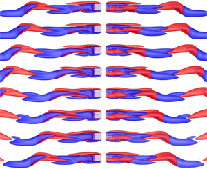
Figure 11. Isosurfaces of the streamwise vorticity with $\omega _x=0.1$ as red and $\omega _x=-0.1$ as blue for the HS1 state at ${{\textit {Re}}}=270$, where ($i_0$)–($i_7$) correspond to the temporal moments marked in figure 10(a). The same wake structure in the region of $y<0$ is plotted as two views in each frame, in which the left and the right ones are about the $x$–$z$ view along the negative and positive $y$-axis, respectively. The streamwise vortex tubes in the $y<0$ region are labelled as $N_3$, $N_4$, $P_1$ and $P_4$ in ($i_0$) and ($i_2$).

It is reasonable to anticipate that, near the critical ${{\textit {Re}}}$ for the Hopf bifurcation, the wake instability is evolved from a steady structure similar to the one shown in figure 6. To be consistent, the labels $P_1$, $P_4$, $N_4$ and $N_3$ are again employed to mark the tubes in figure 11$(i_0)$ and 11$(i_2)$. The strength of the streamwise vortex tubes is expected to increase with increasing ${{\textit {Re}}}$. In order to substantiate this inference, the circulation $\varGamma$ is quantified by integrating the time-averaged streamwise vorticity over the region $\{x=6,-2\le y\le 0,-2\le z\le 2\}$. The circulation contained in a slice of the vortex tube is chosen to represent the circulation contained in the tube is primarily because it is not straightforward to calculate the circulation in the three-dimensional vortex tube. Nonetheless, we find this representation works quite well, as evidenced by the variation trend of $\varGamma$ with ${{\textit {Re}}}$ in the vicinity of Hopf bifurcation shown in figure 10(b). The cut-off value of $\omega _x>-0.0001$ is used to quantify the circulation of the negative streamwise vortex tubes. It is seen from figure 10(b) that the strength of the negative vortex tube (i.e. the absolute value of $\varGamma$) indeed increases with ${{\textit {Re}}}$ as we inferred. The different variation trends of $\varGamma$ in the PSS and HS regimes allow us to determine the critical ${{\textit {Re}}}$ for Hopf bifurcation as the intersection of the two variation trends. The critical ${{\textit {Re}}}$ of 251.3 estimated here is very close to the value of 252.0 determined through Landau's equation to be presented later on in § 6.2.

When ${{\textit {Re}}}>{{\textit {Re}}}_{cr}^{HT}$, the merged tube by $N_4$ with $N_3$ in the domain $y<0$ is incapable of sustaining more circulation, since the vorticity is continuously fed into it from the cube surface. The excessive amount of circulation is accumulated at the downstream end of the merged tube by $N_4$ with $N_3$, forming a section of strong negative vortex tube in $5< x<8$, as shown in figure 11$(i_0)$. The low pressure induced by the section of the strong negative vortex tube tends to draw $P_1$ and $P_4$ towards it, leading to a merging process by $P_1$ with $P_4$ from figure 11$(i_0)$ to 11$(i_4)$. As the merged tube by $P_1$ with $P_4$ gains significant strength, it will cut into the merged tube by $N_4$ with $N_3$ and eventually leads to the shedding of the section of the strong negative vortex tube in figure 11$(i_5)$. The vorticity continues to accumulate in the downstream end of the merged tube by $P_1$ with $P_4$. The low pressure region induced by merged $P_1$ with $P_4$ encourages the merging of $N_4$ with $N_3$, which eventually cuts off the strong positive section of the merged tube by $P_1$ with $P_4$ and leads to its shedding, as shown in figure 11$(i_6)$ and 11$(i_7)$. Then a full vortex shedding cycle is finished. In summary, the regular vortex shedding in the HS1 state is characterised by a process involving the merging, cutting-off and releasing of $N_4$ with $N_3$ and $P_1$ with $P_4$ in the region $y<0$. The same process in the region $y>0$ can be also described by those of $P_2$ with $P_3$ and $N_1$ with $N_2$. The physical mechanism behind this process is that the low pressure induced by the strong section of merged streamwise vortex tubes attracts another two streamwise vortex tubes of opposite signs towards it, and the subsequent merging of the two opposite-sign vortex tubes leads to the shedding of the strong section of merged streamwise vortex tubes. This process happens alternately in two halves of a regular shedding period.

The wake structure at ${{\textit {Re}}}=270$ is further illustrated by the isosurface of $\lambda _2$ in figure 12 (for $\lambda _2$ technique, see Jeong & Hussain Reference Jeong and Hussain1995), where the isosurfaces are coloured by the streamwise vorticity $-0.03<\omega _x<0.03$ varying from blue to red. The flow at the moment $i=7$ in figure 10(a) is only employed to plot the global view in figure 12(a), since the length of the compute domain is enough to display the propagation of hairpin vortices in three full periods, so that the evolution of a hairpin vortex can be approximately traced by comparing these consecutive cycles. The complex interactions of vortex tubes in the wake lead to the unique wake structures observed in figure 12(a), which are distinctly different from those formed in the wake of long cylindrical structures such as circular cylinders and prisms of different cross-section shapes (Thompson et al. Reference Thompson, Hourigan, Ryan and Sheard2006; Sau Reference Sau2009). The shedding process characterised by the merging and cutting-off of streamwise vortex tubes in figure 11 forms upper and lower branches for the hairpin vortices in the wake, as marked in figure 12(a). From the near-wake view in figure 12(b), the streamwise vortex tubes can also be clearly distinguished from the isocontour of $\lambda _2$ around the cube, where only the positive tubes $P_1$ and $P_4$, and the negative ones $N_1$ and $N_2$ are marked accordingly. Further discussions on the dynamics and evolution of the hairpin vortices are not presented here, because it digresses from the topic of this study, while it might be a worthwhile point to form a separated investigation in the future.

Figure 12. Representation of the wake structure at ${{\textit {Re}}}=270$ by isosurfaces of $\lambda _2$ coloured by a blue-white-red colour map of $\omega _x$ varying from $-0.03$ to 0.03, where (a,b) are the global and near-wake structures at the moment $i=7$ in figure 10(a).

5.2.2. Quasi-periodic shedding

The QP state is characterised by the emergence of a dominant low frequency component (${{\textit {St}}}_2$) that modulates the regular oscillations of the lift coefficient observed in the HS1 state. Although the QP state has not been reported before for the laminar wake of a cube, similar phenomena involving modulating frequencies have been found in other bluff-body flows, e.g. Lee (Reference Lee2000) and Tomboulides & Orszag (Reference Tomboulides and Orszag2000) for spheres; Gao et al. (Reference Gao, Tao, Tian and Yang2018) for an inclined circular disk; Bohorquez et al. (Reference Bohorquez, Sanmiguel-Rojas, Sevilla, Jiménez-González and Martinez-Bazan2011) for a slender blunt-based body. The physical origin of ${{\textit {St}}}_2$ along with the shedding of hairpin vortices for the cube is considered by taking advantage of the QP state at ${{\textit {Re}}}=282$, where ${{\textit {St}}}_1 \approx 0.0982$ remains dominant over ${{\textit {St}}}_2 \approx 0.0282$, as shown in figure 9(d). It is noted that ${{\textit {St}}}_1/{{\textit {St}}}_2 \sim 7/2$, corresponding to the occurrence of seven vortex shedding cycles in approximately two secondary periods. This behaviour suggests the state observed here is in the vicinity of a high-order synchronisation of ${{\textit {St}}}_1/{{\textit {St}}}_2 = 7/2$ in the parameter space, where the ratio of two frequencies is a rational number (Pikovsky et al. Reference Pikovsky, Rosenblum and Kurths2003). Previous studies (e.g. Ren et al. Reference Ren, Cheng, Tong, Xiong and Chen2019) have shown that the stroboscopic view of flow fields sampled at the higher frequency over the entire period of the low frequency constitutes an effective way of revealing the physical mechanism of quasi-periodic oscillation. The regular vortex shedding frequency ${{\textit {St}}}_1 \approx 0.0982$ is used as the sampling frequency over the secondary period in the following flow visualisations.

Figure 13(a) exhibits the time history of $C_{{l},z}$ for the case ${{\textit {Re}}}=282$, where eight temporal moments, as marked by the open circles, are uniformly distributed in time under $\Delta t = 1/{{\textit {St}}}_1 \approx 10.18$. The secondary axis $i$ is employed to refer to each moment. It is seen that the phases of the open circles are not identical and $C_{{l},z}$ oscillates around a mean value over the secondary period, confirming the quasi-periodic nature of the flow. The projected $x$–$z$ views of the flow field sampled at those moments are shown in figure 14, where the vortex structure is represented by the isosurface of $\lambda _2$ coloured by the streamwise vorticity $-0.03<\omega _x<0.03$. A remarkable flow feature observed in figure 14 is that the phase at which the head of the lower branch is released into the wake becomes unstable and varies from cycle to cycle, underlying the occurrence of a secondary instability. The phase undergoes two oscillation cycles over seven vortex shedding periods from figures 14$(i_0)$ to 14$(i_7)$, corresponding to ${{\textit {St}}}_1/{{\textit {St}}}_2 \sim 7/2$. This observation allows us to conclude that ${{\textit {St}}}_2$ is induced by a secondary instability associated with temporal evolution of the wake structure behind the cube. The geometry of the hairpin vortices in the wake of ${{\textit {Re}}}=282$ is similar to that of ${{\textit {Re}}}=270$ in figure 12 since ${{\textit {St}}}_1$ is still dominant, while the relatively weak streamwise oscillation by ${{\textit {St}}}_2$ can also be observed as the propagation of the coherent structures in the same magnitude as shown for the release of the heads in figure 14. Identification of the physical origin of this secondary instability based on the flow features at this Reynolds number is not straightforward because the secondary oscillation is relatively weak. We will continue exploring the physical origin of the secondary instability through more numerical examples below.

Figure 13. Selected ranges of time histories of $C_{{l},z}$ for the QP state at (a) ${{\textit {Re}}}=282$ and (b) ${{\textit {Re}}}=285$, where the eight moments under $\Delta t = 1/{{\textit {St}}}_1 \approx 10.18$ for ${{\textit {Re}}}=282$ and the other eight ones under $\Delta t = 1/{{\textit {St}}}_1 \approx 10.27$ for ${{\textit {Re}}}=285$ are marked with open circles and can be referred to by the secondary axis $i$.

Figure 14. Stroboscopic plots for the case at ${{\textit {Re}}}=282$ in the QP state, with ${{\textit {St}}}_1\approx 0.0982$ as the sampling frequency. The near-wake region is characterised by the $x$–$z$ views of the isosurface of $\lambda _2$ in a blue-white-red colour map of $\omega _x$ varying from $-0.03$ to 0.03, and ($i_0$)–($i_7$) correspond to the moments by the open circles in figure 13(a).

An interesting phenomenon is observed between ${{\textit {Re}}} = 282$ and $285$. The secondary frequency ${{\textit {St}}}_2$ becomes the dominant frequency component at ${{\textit {Re}}}=285$ and this dominance over ${{\textit {St}}}_1$ continues to grow with increasing ${{\textit {Re}}}$ thereafter. This observation suggests the secondary instability associated with ${{\textit {St}}}_2$ has become the dominant feature of flow around a cube at ${{\textit {Re}}} \ge 285$. To explore the flow feature associated with ${{\textit {St}}}_2$, the stroboscopic plots of the isosurface of streamwise vorticity in the space of $y<0$, at selected moments marked in figure 13(b), are examined in figure 15. The oscillation of $C_{{l},z}$ sampled at the vortex shedding frequency ${{\textit {St}}}_1$ becomes more pronounced than that shown in figure 13(a), which is consistent with the contrast between the wake structure observed in figures 14 and 15. The wake structures at different moments shown in figure 14 would have been identical if there were not secondary frequency ${{\textit {St}}}_2$. The different wake structures observed in figure 15 are induced by the phase oscillation of the vortex shedding process observed in figure 11. The oscillation of the wake structure can be clearly observed if our focus is placed on the structure enclosed by the dashed rectangle in figure 15$(i_0)$. The positive and negative vortex tubes in $8< x<16$ start to lower down horizontally in the next two vortex shedding periods, before curling to a similar posture to that shown in figure 15$(i_0)$ at a moment between figures 15$(i_3)$ and 15$(i_4)$, completing a cycle of wake oscillation in ${{\textit {St}}}_2$.

Figure 15. Stroboscopic plots for the case at ${{\textit {Re}}}=285$ in the QP state, with ${{\textit {St}}}_1\approx 0.0979$ as the sampling frequency. The isosurfaces of $\omega _x=0.1$ as red and $\omega _x=-0.1$ as blue are presented in the same way as figure 11, where ($i_0$)–($i_7$) correspond to the temporal moments marked in figure 13(b).

The above oscillation process repeats again approximately from figures 15$(i_4)$ to 15$(i_7)$, completing two cycles of wake oscillation within approximately seven periods of vortex shedding. The near-wake structure shown in figure 15 shows an excellent correlation to the phase oscillation of $C_{{l},z}$ sampled at the vortex shedding frequency ${{\textit {St}}}_1$ in figure 13(b) with ${{\textit {St}}}_1/{{\textit {St}}}_2 \sim 7/2$.

5.2.3. High-order synchronised shedding

As ${{\textit {Re}}}$ is further increased, the flow changes from the QP state to the HS2 state which occurs over $289 \le {{\textit {Re}}} \le 305$. One of the unique characteristics in the HS2 state is that ${{\textit {St}}}_1/{{\textit {St}}}_2 = 7/2$, suggesting a high-order synchronisation between flow features associated with ${{\textit {St}}}_1$ and ${{\textit {St}}}_2$. The underlying physics behind the $7/2$ synchronisation is that seven cycles of vortex shedding happen exactly over two secondary periods.

The time history of $C_{{l},z}$ in two typical secondary periods $2T_2=2/{{\textit {St}}}_2\approx 73.86$ is shown in figure 16 for ${{\textit {Re}}}=300$. For the purpose of flow visualisation, the two secondary periods are divided into two uneven periods with $\mathcal {T}_1\approx 40.49$ and $\mathcal {T}_2\approx 33.37$ based on the recurrence pattern of the lift coefficient $C_{{l},z}$. The flow structures are visualised through the isosurfaces of $\omega _x$ in figure 17. In each of $\mathcal {T}_1$ and $\mathcal {T}_2$, 16 moments are selected uniformly, as shown by the open circles in figure 16. All of the moments are plotted for the isosurfaces of $\omega _x$ in figure 17. There are more snapshots of the flow field employed in figure 17 than those shown in previous cases so as to identify the physics behind the secondary oscillation of the wake. The visualisation method employed in figure 17 is the same as that used in figure 11 at ${{\textit {Re}}}=270$.

Figure 16. Time history of $C_{{l},z}$ in two secondary periods $2T_2=\mathcal {T}_1 + \mathcal {T}_2$ for the HS2 state at ${{\textit {Re}}}=300$. The full period $2T_2$ is divided into two portions $\mathcal {T}_1\approx 40.49$ and $\mathcal {T}_2\approx 33.37$ by the recurrence of $C_{{l},z}$, where 16 moments are uniformly selected for each portion, as marked by the open circles. The secondary axis $i$ is employed to refer to every moment.

Figure 17. Isosurfaces of the streamwise vorticity with $\omega _x=0.1$ as red and $\omega _x=-0.1$ as blue for the HS2 state at ${{\textit {Re}}}=300$, where ($i_0$)–($i_{15}$) correspond to the first 16 temporal moments marked within $\mathcal {T}_1$ in figure 16, while ($i_{16}$)–($i_{31}$) correspond to the rest of the 16 moments in $\mathcal {T}_2$. The manner to exhibit the flow structures in figure 11 is employed.

The alternate shedding process of vortex tubes at the initial phases of $\mathcal {T}_1$ is similar to that observed in HS1, as shown by the flow features corresponding to ${{\textit {St}}}_1$ in figure 11. Three pairs of vortex tubes, whose negative and positive branches are marked as $V_1$, $V_2$ and $V_3$, are shed into the wake from figures 17$(i_0)$ to 17$(i_9)$. The flow becomes rather stable after that and only one pair of vortex tubes, marked as $V_4$, is shed between the moments spanning from figures 17$(i_9)$ to 17$(i_{15})$, forming a large peak of $C_{{l},z}$ spanning from $i=9$ to 15 in figure 16. Regular vortex shedding resumes after that with two pairs of vortex tubes $V_5$ and $V_6$ shed from figures 17$(i_{16})$ to 17$(i_{23})$, where the positive branch of $V_4$ is squeezed together with the shedding of $V_5$ in figure 17$(i_{16})$. The flow becomes stable again with only one pair of vortex tubes $V_7$ shed between the moments spanning from figures 17$(i_{23})$ to 17$(i_{31})$, forming another large peak of $C_{{l},z}$ between $i=23$ and $i=31$ in figure 16. It is clear from the above observation that the dominant flow feature associated with ${{\textit {St}}}_2$ is the two relatively stable flow cycles over exactly seven periods of vortex shedding at ${{\textit {St}}}_1$.

The interaction of streamwise vortex tubes appears to be responsible for the relatively stable flow cycles. The vortex tubes $N_4$, $N_3$, $P_1$ and $P_4$ become relatively weak in figure 17$(i_9)$ after the consecutive shedding of three pairs of vortex tubes in figures 17$(i_0)$–17$(i_9)$, and experience an epoch of growth after figure 17$(i_9)$. Subsequently, the fast growth of merged $N_4$ and $N_3$ hinders the growth and merging of $P_1$ and $P_4$ through the cancellation mechanism of vorticity of opposite signs, leading to a substantial delay of the shedding of the merged $N_4$ and $N_3$ in figure 17$(i_{14})$. The delayed shedding process observed at the second half of $\mathcal {T}_2$ is due to the same flow mechanism described above.

The oscillation of the primary recirculation zone for ${{\textit {Re}}}=300$ is examined through the streamlines on the plane $y=0$, as shown in figure 18, where the even values of $i$ in figure 16 are plotted. It is noted that the upper side of the recirculation zone is sustaining during the full shedding period, while the lower side oscillates under the spectrum of the high-order synchronised state, which is similar to the motion of streamlines in the HS1 flow (e.g. figure 18 of Saha Reference Saha2004 and figure 5 of Klotz et al. Reference Klotz, Goujon-Durand, Rokicki and Wesfreid2014).

Figure 18. The periodic variations of the two-dimensional streamlines on the plane $y=0$ at ${{\textit {Re}}}=300$ in the HS2 state, where the moments at even values of $i$ in figure 16 are exhibited in each plot.

5.3. Chaotic shedding

That the flow becomes chaotic has been shown with the case ${{\textit {Re}}}=315$ in figures 9(s)–9(u). As ${{\textit {Re}}}$ is further increased, larger amplitude fluctuations will occur both on $C_{{l},y}$ and $C_{{l},z}$, suggesting the dominant shedding direction switches in the $y$–$z$ plane. To facilitate further discussions, temporal variations of $C_{{l},y}$ and $C_{{l},z}$ at ${{\textit {Re}}}=390$ are examined over three intervals marked by the dashed rectangles in figures 19(a) and 19(b). In the first and second intervals, one of the lift coefficients oscillates around a non-zero value while the other one oscillates around zero, indicating the vortex shedding is in either the $x$–$z$ or $x$–$y$ plane. It is interesting to note that both of the lift coefficients oscillate around non-zero values in the third interval, where $C_{{l},y}$ oscillates around a positive value while $C_{{l},z}$ around a negative one. It is speculated that the primary direction of vortex shedding is in the $y=-z$ plane during this interval. To confirm this speculation, the lift coefficients in the third interval are recalculated by projecting to the diagonal directions, i.e. $\hat {C}_{{l},y} = \sqrt {2}/2 (C_{{l},y} - C_{{l},z})$ and $\hat {C}_{{l},z} = \sqrt {2}/2 ( C_{{l},y} + C_{{l},z})$. The original and transformed lift coefficients are plotted in figures 19(c) and 19(d). We note that the mean values of the original $C_{{l},y}$ and $C_{{l},z}$, i.e. 0.069 and $-0.085$, are close to each other in magnitude and both away from zero in figure 19(c), while the transformed $\hat {C}_{{l},z}$ decreases to a value around zero in figure 19(d). This result basically confirms the above speculation. Since the flow shedding remains nearly in the plane $y=-z$ only briefly, we suspect the flow is relatively unstable on the diagonal planes of $y=z$ and $y=-z$.

Figure 19. Time histories of lift coefficients for the case at ${{\textit {Re}}}=390$, where (a,b) are $C_{{l},y}$ and $C_{{l},z}$ with three distinct intervals marked by the rectangles, (c) is the two lift coefficients in the third interval, and (d) is the lift coefficients by mapping onto the diagonal direction through $\hat {C}_{ {l},y} = \sqrt {2}/2 (C_{ {l},y}-C_{ {l},z})$ and $\hat {C}_{ {l},z} = \sqrt {2}/2 (C_{ {l},y} + C_{ {l},z})$.

To further confirm the above inference, the coherent structures represented by isosurfaces of $\lambda _2$ are exhibited in figure 20, where the hairpin vortices are plotted at three selected moments $t=600$, 1247 and 2101 from the three intervals. Figures 20(a,c,e) and 20(b,d,f) show the $x$–$y$ and $x$–$z$ projected views, respectively. It is clearly observed, in figures 20(a) and 20(b) at $t=600$, that the vortex shedding mainly occurs in the $z$ direction. While, it changes to the $y$ direction in figures 20(c) and 20(d) for $t=1247$, and becomes oblique in figures 20(e) and 20(f) for $t=2101$.

Figure 20. Isosurfaces of $\lambda _2$ at ${{\textit {Re}}}=390$ coloured by the streamwise vorticity $-0.03<\omega _x<0.03$ varying from blue to red, where (a,b) are projected views of the coherent structure on the $x$–$y$ and $x$–$z$ planes for $t=600$, (c,d) are for $t=1247$ and (e,f) are for $t=2101$.

6.1. Regular bifurcation

The nature of the regular and Hopf bifurcations observed in the wake of a cube is investigated through weakly nonlinear analysis in this section. The regular bifurcation from OSS to PSS is a stationary one between two steady states and is believed to be a pitchfork bifurcation, which was also mentioned as a supercritical imperfect bifurcation in Klotz et al. (Reference Klotz, Goujon-Durand, Rokicki and Wesfreid2014). The trajectories of the regular bifurcation in the wake of the cube are bijectively reflected by the growth of the lift coefficients exerted on the cube, as exhibited in figures 7 and 8. The non-dimensional lift force can be characterised by the two-dimensional vector $(C_{{l},y},C_{{l},z})$, which will be disturbed from its equilibria in the vicinity of flow transition from OSS to PSS. Thus, a two-dimensional dynamical system regarding the variation of the $(C_{{l},y},C_{{l},z})$ can be employed to describe the regular bifurcation as follows:

(6.1)\begin{gather} \dfrac{\mathrm{d} C_{{l},y}}{\mathrm{d} t}=f(C_{{l},y},C_{{l},z}), \end{gather}

(6.2)\begin{gather}\dfrac{\mathrm{d} C_{{l},z}}{\mathrm{d} t}=f(C_{{l},z},C_{{l},y}). \end{gather}

The orthogonal symmetry of the flow demonstrates that $(C_{{l},y},C_{{l},z})=(0,0)$ is the only stable fixed point in the OSS regime before it bifurcates to the PSS regime, where the planar symmetry with respect to the plane either $y=0$ or $z=0$ is retained. Due to the symmetry of the cube with respect to the diagonal direction, $C_{{l},y}$ and $C_{{l},z}$ are interchangeable, which guarantees an identical $f(\xi ,\eta )$ in (6.1) and (6.2). Four equilibria at $(\pm C_{l}^{{sat}},0)$ and $(0,\pm C_{l}^{{sat}})$, where $C_{l}^{{sat}}$ denotes the $\ell ^{2}$-norm of the lift coefficients at saturation, are expected based on (6.1) and (6.2). The form of the coupling terms in $f(\xi ,\eta )$ can be determined through Taylor expansion at $(0,0)$ and enforcing symmetry conditions of $(C_{{l},y},C_{{l},z})$ $\to$ $(-C_{{l},y},C_{{l},z})$ and $(C_{{l},y},C_{{l},z})$ $\to$ $(C_{{l},y},-C_{{l},z})$,

(6.3)\begin{equation} f(\xi,\eta)=k_1\xi+k_2\xi^{3}+k_3\xi\eta^{2}+\cdots, \end{equation}

where $k_1$, $k_2$ and $k_3$ are real coefficients and, as to each term $\xi ^{m}\eta ^{n}$, $m+n$ is odd and $n$ has to be even.

Substituting (6.3) into (6.1) and (6.2) and omitting high-order terms, we have

(6.4)\begin{gather} \dfrac{\mathrm{d} C_{{l},y}}{\mathrm{d} t}=C_{{l},y}[k_1+k_2(C_{{l},y}^{2}+\gamma C_{{l},z}^{2})], \end{gather}

(6.5)\begin{gather}\dfrac{\mathrm{d} C_{{l},z}}{\mathrm{d} t}=C_{{l},z}[k_1+k_2(C_{{l},z}^{2}+\gamma C_{{l},y}^{2})], \end{gather}

where $\gamma =k_3/k_2$. Eight non-trivial equilibria for $(C_{{l},y},C_{{l},z})$ can be obtained from (6.4) and (6.5),

(6.6)\begin{gather} \left({\pm} \sqrt{-\dfrac{k_1}{k_2}},0 \right), \left(0, \pm \sqrt{-\dfrac{k_1}{k_2}}\right) , \end{gather}

(6.7)\begin{gather}\left({\pm} \sqrt{-\dfrac{k_1}{k_2(1+\gamma)}},\pm \sqrt{-\dfrac{k_1}{k_2(1+\gamma)}}\right), \left({\pm} \sqrt{-\dfrac{k_1}{k_2(1+\gamma)}}, \mp \sqrt{-\dfrac{k_1}{k_2(1+\gamma)}}\right). \end{gather}

The stability of the coupled pitchfork system at these equilibria can be further examined by linear stability analysis. By applying the variational operation to (6.4) and (6.5), the corresponding Jacobian matrix can be derived as

(6.8)\begin{equation} \boldsymbol{J}(C_{{l},y},C_{{l},z})=\left(\begin{array}{cc} k_1 + k_2(3C_{{l},y}^{2}+\gamma C_{{l},z}^{2}) & 2\gamma k_2C_{{l},y}C_{{l},z} \\ 2\gamma k_2C_{{l},z}C_{{l},y} & k_1 + k_2(3C_{{l},z}^{2}+\gamma C_{{l},y}^{2}) \end{array} \right). \end{equation}

The equilibrium $(0,0)$ is known as unstable in PSS. Therefore, the eigenvalues of $\boldsymbol {J}(0,0)$ denoted as $\lambda _{1,2}=k_1$ should be positive, i.e. $k_1>0$. Without loss of generality, we take $(0,\sqrt {-k_1/k_2})$ as the fixed point $(0,C_{l}^{{sat}})$. It is thus required that $k_2<0$ and the eigenvalues of $\boldsymbol {J}(0,\sqrt {-k_1/k_2})$ derived as $\lambda _1=-2k_1$ and $\lambda _2=k_1(1-\gamma )$ are both negative, which results in $\gamma >1$. The determinate signs of $k_2$ and $\gamma$ imply that the third-order nonlinear terms stabilise the coupled pitchfork bifurcation system and the nature of the regular transition in the wake of the cube is supercritical. Through the same reasoning, the stability of the diagonal equilibria in (6.7) can be shown as saddle points, suggesting the existence of the alternative PSS regime with respect to the diagonals are impossible in the wake of the cube.

The time histories of $C_{{l},y}$ and $C_{{l},z}$ at ${{\textit {Re}}} = 210$, which is slightly above the critical ${{\textit {Re}}}$ value of the bifurcation from OSS to PSS, are plotted in figure 21(a) to quantify the value of $k_2$. The linear forms of (6.4) and (6.5) can be written as

(6.9)\begin{gather} \dfrac{\mathrm{d} \ln C_{{l},y}}{\mathrm{d} t}=k_1+k_2(C_{{l},y}^{2}+\gamma C_{{l},z}^{2}), \end{gather}

(6.10)\begin{gather}\dfrac{\mathrm{d} \ln C_{{l},z}}{\mathrm{d} t}=k_1+k_2(C_{{l},z}^{2}+\gamma C_{{l},y}^{2}). \end{gather}

The dependence of ($\mathrm {d}\ln C_{{l},y}/\mathrm {d}t$) on ($C_{{l},y}^{2}+\gamma C_{{l},z}^{2}$) and ($\mathrm {d}\ln C_{{l},z}/\mathrm {d}t$) on $(C_{{l},z}^{2}+\gamma C_{{l},y}^{2}$) is tested by assuming different values of $\gamma$ in (6.9) and (6.10) and the corresponding results are plotted in figures 21(b) and 21(c). Both equations become approximately linear at $\gamma \approx 1.435$, which leads to $k_1\approx 0.00572$ and $k_2\approx -8.43$ deduced via linear fitting.

Figure 21. (a) Time histories of $C_{{l},y}$ and $C_{{l},z}$ either by the DNS results at ${{\textit {Re}}}=210$ or by the prediction of the coupled pitchfork bifurcation model; (b) the linear dependence of ($\mathrm {d}\ln {C_{{l},y}} / \mathrm {d}t$) on ($C_{{l},y}^{2} + \gamma C_{{l},z}^{2}$); (c) the linear dependence of ($\mathrm {d}\ln {C_{{l},z}}/ \mathrm {d}t$) on ($C_{{l},z}^{2} + \gamma C_{{l},y}^{2}$); (d) the trajectories with stable, saddle and unstable equilibria of the coupled pitchfork model in the phase space.

With this set of control parameters at ${{\textit {Re}}}=210$, the predictions of time histories of $(C_{{l},y},C_{{l},z})$ based on (6.4) and (6.5) with an initial perturbation of $(0.835,1.07) \times 10^{-5}$ are plotted in figure 21(a), and the possible trajectories in phase space $C_{{l},y}$–$C_{{l},z}$ is demonstrated in figure 21(d). The predictions based on the two-dimensional coupled pitchfork model are in good agreement with the simulation results. The four stable fixed points located on the axes and the four saddle nodes on the diagonals are clearly observed through those trajectories.

The supercritical nature of the bifurcation from OSS to PSS implies that any infinitesimal disturbances will initiate the flow bifurcation from OSS to PSS when the Reynolds number is slightly greater than the critical value. Thus, the critical value of Reynolds number for the regular transition, denoted as ${{\textit {Re}}}_{cr}^{RT}$, can be estimated as the point where the linear growth rate $k_1$ changes its sign. Figure 22 illustrates the linear initial stage of $\ln C_{l}$ for four cases in the vicinity of the regular transition and the dependence of the growth rate on ${{\textit {Re}}}$. The critical value of ${{\textit {Re}}}_{cr}^{RT}\approx 207.0$ is obtained through a linear correlation of the growth rate with ${{\textit {Re}}}$.

Figure 22. (a) Time histories of $\ln C_{l}$ at ${{\textit {Re}}}=200$ and 205 for the OSS2 state and ${{\textit {Re}}}=210$ and 215 for the PSS state; (b) the linear relation regarding the growth rate of $C_{l}$ as the increase of Reynolds number, where the critical Reynolds number for the regular transition ${{\textit {Re}}}_{cr}^{RT}$ is estimated at 207.0 by interpolation.

6.2. Hopf bifurcation

The nature of the Hopf bifurcation from PSS to HS1 is considered below. At the onset of the HS1 state, a pair of complex eigenvalues should emerge to govern the growth of disturbance, for which Landau's equation has been proven appropriate to describe this nonlinear dynamical behaviour (Stuart Reference Stuart1960; Watson Reference Watson1960) as

(6.11)\begin{equation} \dfrac{\mathrm{d} Z}{\mathrm{d} t} = c_1 Z + c_2 |Z|^{2} Z+ \cdots, \end{equation}

where $Z=|Z|{\rm e}^{{\rm i}\phi }$ represents the complex disturbance of interest, with $|Z|$ and $\phi$ being its amplitude and phase, respectively; $c_i=a_i+{\rm i}b_i$ is the complex coefficient. In particular, $a_2$ is the first Lyapunov coefficient.

Substituting the expression of $Z$ into (6.11), the temporal variation of the amplitude and phase are decoupled, such that we obtain an equation with respect to $|Z|$ in the form of

(6.12)\begin{equation} \dfrac{\mathrm{d}\ln |Z|}{\mathrm{d} t} = a_1 + a_2 |Z|^{2} + \cdots. \end{equation}

With the similar criterion to the pitchfork bifurcation, the nature of the Hopf bifurcation can be determined by the sign of the first Lyapunov coefficient $a_2$. Figure 23(a) shows the time histories of the lift coefficients at ${{\textit {Re}}}=255$, which is slightly greater than the critical value ${{\textit {Re}}}$ for the Hopf bifurcation. The two characteristic dynamical behaviours displayed by the time histories of the lift coefficients, namely the rapid decay of $C_{{l},y}$ to zero and the growth of $C_{{l},z}$ to a periodic pattern for $t > 300$, are somewhat expected. The rapid decay of $C_{{l},y}$ to zero suggests the flow symmetry about the plane $y=0$ is retained in HS1, while the growth of $C_{{l},z}$ to the periodic pattern implies that the regular vortex shedding occurs in the $x$–$z$ plane. Based on the results shown in figure 23(a), the time history of $C_{{l},z}$ for $t> 300$ is selected for the consideration of Landau's equation, and the amplitude is extracted by means of

(6.13)\begin{equation} |Z| = \dfrac{\text{upper envelope}-\text{lower envelope}}{2}. \end{equation}

The relation between $\mathrm {d}\ln |Z|/\mathrm {d}t$ and $|Z|^{2}$ is calculated in figure 23(b), in which a linear dependence is subsequently established with a negative slope, such that the sign of $a_2$ is recognised. Therefore, the Hopf bifurcation is determined as supercritical, which is consistent with Klotz et al. (Reference Klotz, Goujon-Durand, Rokicki and Wesfreid2014), and the wakes of a sphere (Thompson, Leweke & Provansal Reference Thompson, Leweke and Provansal2001) and ring tori (Sheard, Thompson & Hourigan Reference Sheard, Thompson and Hourigan2004).

Figure 23. (a) Time histories of $C_{{l},y}$ and $C_{{l},z}$ with the employed upper and lower envelopes at ${{\textit {Re}}}=255$; (b) the linear correlation between $\mathrm {d}\ln {|Z|} / \mathrm {d}t$ and $|Z|^{2}$.

The critical Reynolds number for the transition from PSS to HS1, denoted as ${{\textit {Re}}}_{cr}^{HT}$, is estimated by correlating the growth rate with $Re$ in the vicinity of the transition point from ${{\textit {Re}}}=245$ to 255. For the cases with ${{\textit {Re}}}<{{\textit {Re}}}_{cr}^{HT}$, artificial perturbations are introduced to disturb the flows at ${{\textit {Re}}}=245$ and 250 in order to obtain the growth rate. The steady solution of the flow at ${{\textit {Re}}}=240$ is used as the initial condition for the simulations at ${{\textit {Re}}}=245$ and 250. The envelops employed to calculate the growth rate at ${{\textit {Re}}}=245$ are exhibited in figures 24(a) and 24(b), and those for ${{\textit {Re}}}=250$ are in figures 24(c) and 24(d). The amplitude of each envelope $|Z|$ is derived by the same expression in (6.13), and the variations of $\ln |Z|$ against $t$ are plotted in figures 24(e) and 24(f) for ${{\textit {Re}}}=245$ and 250, respectively. A linear correlation shown in figure 24(g) suggests ${{\textit {Re}}}_{cr}^{HT} \approx 252.0$.

Figure 24. Linear interpolation for the critical Reynolds number of Hopf transition: (a–d) the time histories of lift coefficients for ${{\textit {Re}}}=245$ and 250 obtained by using ${{\textit {Re}}}=240$ at $t=516$ as the initial flow state; (e,f) are the linear relations between the amplitude $\ln |Z|$ and $t$; (g) the growth rates for cases in the vicinity of the Hopf transition, where the critical value ${{\textit {Re}}}_{{cr}}^{{HT}}$ is estimated at 252.0 by interpolation.

6.3. Global bifurcation features

Global bifurcation features of flow around a cube are examined by plotting peak values of $C_{{l},y}$ and $C_{{l},z}$ in figure 25 over the range of ${{\textit {Re}}}$ investigated in the present study. Since the peak values of $C_{{l},y}$ and $C_{{l},z}$ are extracted from temporal variations of $C_{{l},y}$ and $C_{{l},z}$ over a long period of simulation time (at least five periods for $255\le {{\textit {Re}}}\le 305$ and 1500 time units for $310\le {{\textit {Re}}}\le 400$), figure 25 actually represents a phase diagram in ${{\textit {Re}}}$ space. The global bifurcation is characterised by different types of attractors. In the OSS regime, which includes the NS, OSS1 and OSS2 states, the attractors are fixed points at $(C_{{l},y}, C_{{l},z}) = (0,0)$. The attractor is a fixed point at $(0, C_{{l},z})$ in the PSS regime. In the HS1 state the time history of $C_{{l},z}$ starts to oscillate between two local extrema periodically. Therefore, the stable orbit of $C_{{l},z}$ settles into a limit circle with a non-zero mean of $C_{{l},z}$. The limit circle of $C_{{l},z}$ is distorted by the emerging secondary instability in the QP state. The two branches of local maxima and minima are scattered into inconsistent values. With the periodicity re-established in the form of high-order synchronisations in the HS2 state, the dispersed characteristic values of $C_{{l},z}$ return to a finite number of consistent values again, corresponding to that the limit torus collapses to well-defined limit circles in the HS2 state. The cascade of period-doubling and period-halving bifurcations is qualitatively reflected on the number of local maxima and minima of $C_{{l},z}$ at different Reynolds numbers. In the CS regime the flow is governed by chaotic attractors, such that both $C_{{l},y}$ and $C_{{l},z}$ start to oscillate randomly with the breaking of planar symmetry with respect to the $y=0$ plane.

Figure 25. Bifurcation diagram by the stable orbits of the lift coefficients in all recognised flow states and regimes.

The evolution of the mean drag coefficient $\overline {C_{d}}$, the length of the primary recirculation zone $l_1$ and the Strouhal numbers ${{\textit {St}}}_1$ and ${{\textit {St}}}_2$ with ${{\textit {Re}}}$ are illustrated in figures 26(a), 26(b) and 26(c), respectively. The mean drag coefficient $\overline {C_{d}}$ experiences a monotonic decrease with increasing ${{\textit {Re}}}$ until ${{\textit {Re}}} \approx 310$, which coincides with the onset of the CS regime. In the CS regime, $\overline {C_{d}}$ increases slightly with increasing ${{\textit {Re}}}$. This trend of $\overline {C_{d}}$ against ${{\textit {Re}}}$ is apparently different with that of freely moving cubes, where $\overline {C_{d}}$ will first decrease as the drag coefficient of the fixed cube in lower Reynolds numbers and then experience a sudden increase approximately at ${{\textit {Re}}}=150\text {--}200$ (e.g. Haider & Levenspiel Reference Haider and Levenspiel1989; Tran-Cong, Gay & Michaelides Reference Tran-Cong, Gay and Michaelides2004; Seyed-Ahmadi & Wachs Reference Seyed-Ahmadi and Wachs2019). This is because additional degrees of freedom for the cube leads to a wake transition into helical settling trajectories (Seyed-Ahmadi & Wachs Reference Seyed-Ahmadi and Wachs2019). The length of the primary recirculation zone $l_1$, defined by the maximal $x$ coordinate on the isosurface of $\overline {u_x}=0$, is employed to characterise the mean size of the vortex bubble behind the cube. This definition is equivalent to that by Klotz et al. (Reference Klotz, Goujon-Durand, Rokicki and Wesfreid2014), where the distance from the centre of the cube to the location of the streamwise velocity changing its sign was defined as $l_1$. The $l_1$ variation illustrated in figure 26(b) shows a monotonic increasing trend until the onset of Hopf bifurcation at ${{\textit {Re}}}_{cr}^{HT} \approx 252.0$, a linearly decreasing trend in the HS1 state over $255\le {{\textit {Re}}}\le 280$, a near constant value in the QP and HS2 states over $282\le {{\textit {Re}}}\le 305$, and an irregular variation trend in the CS regime for $310\le {{\textit {Re}}}\le 400$. The Strouhal numbers shown in figure 26(c), due to the strong spectral leakage in the CS regime, are calculated based on the streamwise velocity at $(3,0,0)$ and represented by the largest values among multiple peaks around $f=0.1$ for ${{\textit {St}}}_1$ and $f=0.025$ for ${{\textit {St}}}_2$. It is noted that the values of ${{\textit {St}}}_1$ and ${{\textit {St}}}_2$ are both slightly increased in HS1 but exhibit decreasing trends in QP and HS2. However, in the CS regime for $310\le {{\textit {Re}}}\le 400$, ${{\textit {St}}}_1$ and ${{\textit {St}}}_2$ turn to be obviously increasing against ${{\textit {Re}}}$.

Figure 26. (a) The time-averaged drag coefficients $\overline {C_{d}}$ against ${{\textit {Re}}}$; (b) the length of the primary recirculation zone $l_1$ against ${{\textit {Re}}}$, where $l_1$ is defined by the maximal $x$ coordinate on the isosurface of $\overline {u_x}=0$; (c) the Strouhal numbers ${{\textit {St}}}_1$ and ${{\textit {St}}}_2$ against ${{\textit {Re}}}$ in the unsteady regimes.