


1. Introduction
Flow tones generated by shear layers interacting with solid surfaces have been studied for decades, however, investigating these problems can still provide a substantial advance in our understanding of vortical–acoustic interaction. With a shear flow past an open cavity, self-sustained oscillations can happen owing to the feedback-loop mechanism that is usually attributed to Rossiter (Reference Rossiter1964): the spatially growing Kelvin–Helmholtz (KH) instability wave scatters into acoustic waves at the downstream edge, and acoustic waves propagate upstream and excite the new instability wave. Rossiter also obtained a semi-empirical formula for oscillation frequencies based on the phase relation of the feedback loop. Essentially the same feedback-loop mechanism was known earlier in jet edge tones (Powell Reference Powell1953, Reference Powell1961). Powell has examined not only the loop phase relation, but also the loop gain (the loop amplitude relation) which is relevant to whether self-sustained oscillations happen or not at the frequencies determined by the phase requirement. The original feedback-loop idea has been credited to Lord Rayleigh (see Powell Reference Powell1995), who described the mechanism of a high-pitched whistle called a bird call (Rayleigh Reference Rayleigh1945). Over the past decades, such a feedback-loop mechanism has been found to be responsible for many tonal flows, such as cavity flows and impinging jets (see reviews such as Rockwell & Naudascher (Reference Rockwell and Naudascher1978), Blake & Powell (Reference Blake and Powell1986), Fabre & Hirschberg (Reference Fabre and Hirschberg2000), Rowley & Williams (Reference Rowley and Williams2006), Gloerfelt (Reference Gloerfelt2009), Tonon et al. (Reference Tonon, Golliard, Hirschberg and Ziada2011), Edgington-Mitchell (Reference Edgington-Mitchell2019)).
In a cavity flow, the free shear layer spanning the cavity is perturbed by the feedback acoustic disturbances (Ho & Huerre Reference Ho and Huerre1984). At low Mach numbers, the acoustic excitation is only effective near the separation point where vortical disturbances are generated, owing to the mismatch between the wavelengths of acoustic and instability waves. The later vortical motions between the separation point and the downstream solid surface, which may appear as spatially growing instability waves in some cases or as concentrated vortex structures in others, largely depend on the initial acoustic excitation (Bauerheim, Boujo & Noiray Reference Bauerheim, Boujo and Noiray2020).
The upstream feedback is not limited to acoustic waves that are associated with the compressibility of fluids, it can be truly hydrodynamic. Incompressible cavity flow oscillations have been observed in experiments, which show similar feedback-loop features as described in the Rossiter model (Knisely & Rockwell Reference Knisely and Rockwell1982; Gharib & Roshko Reference Gharib and Roshko1987). The existence of purely hydrodynamic resonances has been confirmed by incompressible global mode calculations (Barbagallo, Sipp & Schmid Reference Barbagallo, Sipp and Schmid2009; Yamouni, Sipp & Jacquin Reference Yamouni, Sipp and Jacquin2013). At very low Mach numbers, the whole self-sustained system is in the very near field, i.e. the configuration is small compared with the acoustic wavelength (acoustically compact), a hydrodynamic description is also applicable (Powell Reference Powell1961; Ffowcs-Williams Reference Ffowcs-Williams1969; Crighton Reference Crighton1992; Howe Reference Howe1997). In this regime, the upstream feedback might be designated as pseudo-sound (Ffowcs-Williams Reference Ffowcs-Williams1969). Following Goldstein (Reference Goldstein1978), the irrotational feedback disturbances are still referred to as acoustic in this article even though they can be supported by an incompressible model. The designation ‘acoustic’ distinguishes those irrotational disturbances from vortical disturbances that are associated with flow shear. In incompressible or compact cases, since the phase relation of the feedback loop is mainly determined by the vortical motions in the shear layers, the oscillation frequency is roughly proportional to the flow velocity, following the Strouhal law.
The feedback loop consisting of KH instability waves and the Rayleigh–Powell–Rossiter (RPR) feedback can be dramatically influenced by an acoustic resonant mode of the cavity, the Rossiter formula then fails to predict oscillation frequencies (East Reference East1966; Tam & Block Reference Tam and Block1978). Experimental results of such an influence were typically obtained at low flow speeds, and the oscillation frequencies have been shown to deviate from the expected Strouhal law (Nelson, Halliwell & Doak Reference Nelson, Halliwell and Doak1981; Bruggeman et al. Reference Bruggeman, Hirschberg, van Dongen and Wijnands1991; Kook & Mongeau Reference Kook and Mongeau2002; Ma, Slaboch & Morris Reference Ma, Slaboch and Morris2009; Dai, Jing & Sun Reference Dai, Jing and Sun2015). In some cases, it appears that the resonator almost completely imposes its resonant frequencies on the whole self-sustained system (Ziada & Shine Reference Ziada and Shine1992; Peters Reference Peters1993; Kriesels et al. Reference Kriesels, Peters, Hirschberg, Wijnands, Iafrati, Riccardi, Piva and Bruggeman1995; Tonon et al. Reference Tonon, Golliard, Hirschberg and Ziada2011), which is often referred to as frequency lock in. The influence of the resonator also leads to intense self-sustained oscillations and concentrated vortex structures. Similar phenomena happen in many other configurations, such as a flow duct containing plates (Parker Reference Parker1966; Stoneman et al. Reference Stoneman, Hourigan, Stokes and Welsh1988) and a compressor (Hellmich & Seume Reference Hellmich and Seume2008), leading to an extensive study of acoustic resonance without flow in open systems (Hein, Hohage & Koch Reference Hein, Hohage and Koch2004; Koch Reference Koch2009; Hein, Koch & Nannen Reference Hein, Koch and Nannen2012).
The flow-tone problem sketched in figure 1 is considered in this article. Two types of approaches can be used in studying the self-sustained flow oscillations, where shear flows are respectively described as vorticity fields in physical space and hydrodynamic instability waves in Fourier space (Ho & Huerre Reference Ho and Huerre1984). The first approach, such as using the vortex particle method to model shear layer motions (Peters Reference Peters1993; Kriesels et al. Reference Kriesels, Peters, Hirschberg, Wijnands, Iafrati, Riccardi, Piva and Bruggeman1995; Dai et al. Reference Dai, Jing and Sun2015), gives the nonlinear evolution of the shear layers, which can be compared with flow-visualization studies. In the second approach, the examination of the linear tonal dynamics of shear flows is achieved by global mode analyses (Sipp et al. Reference Sipp, Marquet, Meliga and Barbagallo2010; Theofilis Reference Theofilis2011; Yamouni et al. Reference Yamouni, Sipp and Jacquin2013; Fosas de Pando, Schmid & Sipp Reference Fosas de Pando, Schmid and Sipp2014). It is very often that global modes need to be numerically solved from global eigenvalue problems when solid surfaces and mean flows are complex. For a complete understanding of vortical–acoustic coupling and global instabilities here, a combined local–global analysis with a simplified flow model (Gallaire & Chomaz Reference Gallaire and Chomaz2004; Doaré & de Langre Reference Doaré and de Langre2006; Stewart, Waters & Jensen Reference Stewart, Waters and Jensen2009) is also desirable. Thus, the present global modes are constructed from travelling vortical and acoustic waves by the feedback-loop closure principle (Landau & Lifshitz Reference Landau and Lifshitz1981) described in § 2, under the assumption of a parallel mean flow. Such a closure principle reflects the idea of Rayleigh, Powell and Rossiter for global instabilities and the consequent self-sustained oscillations, and it embraces cases whether or not a resonator is present (Powell Reference Powell1990).

Figure 1. Sketches of vortical–acoustic resonance at low flow speeds in two-dimensional (2-D) symmetric duct–cavity configurations, where the flow duct is infinitely long. (a) A shallow-cavity case with a compact  $\textrm {KH}+\textrm {RPR}$ feedback loop, (b) a deep-cavity case where the compact
  $\textrm {KH}+\textrm {RPR}$ feedback loop is affected by the resonator acoustics. The symmetric and antisymmetric (breathing and flapping) KH modes of the jet profile (Tam & Norum Reference Tam and Norum1992; Gojon, Bogey & Marsden Reference Gojon, Bogey and Marsden2016; Martini, Cavalieri & Jordan Reference Martini, Cavalieri and Jordan2019) in the cavity segment are respectively sketched in (a) and (b).
The main objective of this article is to examine the influence of an acoustic resonator (AR) on the  $\textrm {KH}+\textrm {RPR}$ feedback loop. It has been shown that a linear global mode analysis can predict interesting phenomena and provide insight into the influence of an AR on global instabilities and self-sustained oscillations (Alvarez & Kerschen Reference Alvarez and Kerschen2005; Méry Reference Méry2010; Yamouni et al. Reference Yamouni, Sipp and Jacquin2013). For example, an overshoot in temporal growth rate and a global mode switching happen near the frequency of some acoustic resonant modes (Yamouni et al. Reference Yamouni, Sipp and Jacquin2013). For a better understanding of the global mode-related phenomena, a combined travelling–global mode analysis is performed in the present study, taking full advantage of the feedback-loop closure principle. The research plan is as follows. First, the compact case sketched in figure 1(a) is considered in § 3.1, serving as a baseline for comparison. It is noted that a compact case was analysed in Dai (Reference Dai2020), with a compressible model. Here, a purely hydrodynamic feedback loop supported by an incompressible model is demonstrated and compared with the compressible results. Then, two acoustic resonant modes for the deep-cavity case in figure 1(b) but without flow are calculated in § 3.2. The antisymmetric one is a trapped mode which is decoupled from the outgoing propagative travelling modes in the ducts, corresponding to an acoustic resonance with a high quality factor (Pagneux Reference Pagneux2013). The symmetric one is a heavily damped mode owing to radiation. Finally, the vortical–acoustic resonance sketched in figure 1(b) is discussed in § 3.3. Different impacts of the trapped and heavily damped acoustic modes on the global modes are shown. Phenomena such as frequency deviation from the Strouhal law, global mode switching, global mode destabilization and stabilization are explained by the local–global relation of the feedback loop and the dual-feedback view (Powell Reference Powell1990; Fabre & Hirschberg Reference Fabre and Hirschberg2000; Rienstra & Hirschberg Reference Rienstra and Hirschberg2018): the coexistence of RPR and AR feedbacks. Note that antisymmetric and symmetric respectively denote
  $y$-antisymmetric and
  $y$-symmetric in this article.
2. Numerical model
Calculations of vortical–acoustic resonant modes (also called global modes) and acoustic resonant modes are rather simple here. The global mode calculation has been described in Dai (Reference Dai2020) for a compact case, and it is outlined in this section. The duct–cavity configuration is divided into three zones, as shown in figure 1(a): the left semi-infinite duct (zone I), the cavity segment (zone II) and the right semi-infinite duct (zone III). In each zone, duct modes travelling in the  $\pm x$ directions are first solved (Kooijman et al. Reference Kooijman, Testud, Aurégan and Hirschberg2008; Kooijman, Hirschberg & Aurégan Reference Kooijman, Hirschberg and Aurégan2010). The resonant modes are then constructed from the travelling duct modes by the feedback-loop closure principle between the two ends of the cavity segment.
2.1. Governing equations and calculations of travelling duct modes
The linear propagation of vortical and acoustic disturbances in each zone about a parallel mean shear flow is described by the linearized Euler equations (LEEs)
 \begin{gather} \left(\frac{\partial}{\partial t}+M_0f\frac{\partial}{\partial x}\right)u+M_0\frac{\mathrm{d} f}{\mathrm{d} y}v={-}\frac{\partial p}{\partial x}, \end{gather}
 \begin{gather}\left(\frac{\partial}{\partial t}+M_0f\frac{\partial}{\partial x}\right)v ={-}\frac{\partial p}{\partial y}, \end{gather}
 \begin{gather}\left(\frac{\partial}{\partial t}+M_0f\frac{\partial}{\partial x}\right)p ={-}\left(\frac{\partial u}{\partial x}+\frac{\partial v}{\partial y}\right), \end{gather}
where  $u$ and
  $v$ are the velocity disturbance in respectively the
  $x$- and
  $y$-directions,
  $p$ is the pressure disturbance,
  $M_0$ is the average Mach number in the duct with the profile prescribed by the function
  $f(y)=M(y)/M_0$ (the assumed velocity profile of the low-speed mean flow is described at the beginning of § 3.1) and all variables have been normalized by sound speed
  $c_0^*$ and density
  $\rho _0^*$ and the duct height
  $H^*$. The stars in this article denote dimensional quantities, whereas quantities without star are dimensionless.
The fluctuations are sought in the form
 \begin{equation} \left.\begin{gathered} p = P(y)\exp(-\mathrm{i} k x)\exp(\mathrm{i} \omega t ),\\ v = V(y )\exp(-\mathrm{i} k x )\exp(\mathrm{i} \omega t), \end{gathered}\right\} \end{equation}
where  $\mathrm {i}^2=-1$,
  $k$ is the wavenumber and
  $\omega$ is the angular frequency. Inserting (2.4) into the LEEs leads to
 \begin{gather} \mathrm{i} (\omega -M_0\, f\kern0.06em k )V={-}\frac{\mathrm{d} P}{\mathrm{d} y }, \end{gather}
 \begin{gather}\left(1-M_0^2\, f^2 \right) k^2 P+2 \omega M_0 \, f\kern0.06em k P - \omega ^2 P-\frac{\mathrm{d}^2 P}{\mathrm{d} y^2}={-}2 \mathrm{i} M_0 \frac{\mathrm{d} f}{\mathrm{d}y}k V. \end{gather}
 In each zone, vortical and acoustic travelling modes are solved by discretizing (2.5) and (2.6) in the  $y$-direction, taking
  $N_1$ equally spaced points in zones I and III,
  $N_2$ equally spaced points in zone II. The spacing between interior points in all zones is
  $\Delta h =H/N_1= (2D+H)/N_2$, and the first and last points are taken
  $\Delta h/2$ from the solid walls. Equations (2.5) and (2.6), together with the wall boundary conditions, determine the following generalized eigenvalue problem in each zone:
 \begin{align} k \left(\begin{array}{@{}ccc@{}}
\boldsymbol{\mathsf{I}}-M_0^2\boldsymbol{\mathsf{f}}_2
& 2 \mathrm{i} M_0\boldsymbol{\mathsf{f}}_a &
\boldsymbol{\mathsf{0}}\\ \boldsymbol{\mathsf{0}}
& \mathrm{i} M_0\boldsymbol{\mathsf{f}} &
\boldsymbol{\mathsf{0}}\\ \boldsymbol{\mathsf{0}}
& \boldsymbol{\mathsf{0}} &
\boldsymbol{\mathsf{I}} \end{array}
\right)\left(\begin{array}{@{}c@{}} \boldsymbol{Q}\\
\boldsymbol{V}\\ \boldsymbol{P} \end{array}\right)
=\left(\begin{array}{@{}cccc@{}} -2 \omega
M_0\boldsymbol{\mathsf{f}} &
\boldsymbol{\mathsf{0}} & \omega^2
\boldsymbol{\mathsf{I}}+\boldsymbol{\mathsf{D}}_2\\
\boldsymbol{\mathsf{0}} & \mathrm{i} \omega
\boldsymbol{\mathsf{I}} &
\boldsymbol{\mathsf{D}}_1\\
\boldsymbol{\mathsf{I}} & \boldsymbol{\mathsf{0}}
& \boldsymbol{\mathsf{0}} \end{array} \right)
\left(\begin{array}{@{}c@{}} \boldsymbol{Q}\\ \boldsymbol{V}\\
\boldsymbol{P} \end{array} \right),
\end{align}
\begin{align} k \left(\begin{array}{@{}ccc@{}}
\boldsymbol{\mathsf{I}}-M_0^2\boldsymbol{\mathsf{f}}_2
& 2 \mathrm{i} M_0\boldsymbol{\mathsf{f}}_a &
\boldsymbol{\mathsf{0}}\\ \boldsymbol{\mathsf{0}}
& \mathrm{i} M_0\boldsymbol{\mathsf{f}} &
\boldsymbol{\mathsf{0}}\\ \boldsymbol{\mathsf{0}}
& \boldsymbol{\mathsf{0}} &
\boldsymbol{\mathsf{I}} \end{array}
\right)\left(\begin{array}{@{}c@{}} \boldsymbol{Q}\\
\boldsymbol{V}\\ \boldsymbol{P} \end{array}\right)
=\left(\begin{array}{@{}cccc@{}} -2 \omega
M_0\boldsymbol{\mathsf{f}} &
\boldsymbol{\mathsf{0}} & \omega^2
\boldsymbol{\mathsf{I}}+\boldsymbol{\mathsf{D}}_2\\
\boldsymbol{\mathsf{0}} & \mathrm{i} \omega
\boldsymbol{\mathsf{I}} &
\boldsymbol{\mathsf{D}}_1\\
\boldsymbol{\mathsf{I}} & \boldsymbol{\mathsf{0}}
& \boldsymbol{\mathsf{0}} \end{array} \right)
\left(\begin{array}{@{}c@{}} \boldsymbol{Q}\\ \boldsymbol{V}\\
\boldsymbol{P} \end{array} \right),
\end{align}
where  $Q=k P$ is assumed,
  $\boldsymbol{\mathsf{I}}$ is the identity matrix,
  $\boldsymbol{\mathsf{f}}$,
  $\boldsymbol{\mathsf{f}}_2$ and
  $\boldsymbol{\mathsf{f}}_a$ are diagonal matrices with on the diagonal the values of
  $f$,
$f$,  $f^2$ and
  $\mathrm {d} f/\mathrm {d} y$ at the discrete points;
  $\boldsymbol {Q}$,
  $\boldsymbol {V}$ and
  $\boldsymbol {P}$ are the column vectors giving respectively the value of
  $Q(y)$,
  $V(y)$ and
  $P(y)$ at the discrete points;
  $\boldsymbol{\mathsf{D}}_1$ and
  $\boldsymbol{\mathsf{D}}_2$ are matrices for the first- and second-order differential operators with respect to
  $y$. The boundary condition
  $\mathrm {d} p /\mathrm {d} y=0$ on the solid walls is taken into account in the differential operator matrices by introducing ghost points outside the walls. The eigenvalue problems for the duct modes are then solved, using the eig function of MATLAB. In zones I and III,
  $3N_1$ modes are obtained, including
  $N_1$ acoustic modes travelling in the
  $\pm x$ directions and
  $N_1$ vortical modes travelling in the
  $+x$ direction with the mean flow. In zone II, the mean flow velocity and its derivative are zero at discrete points where
  $|y| >H/2$. The first and last
  $(N_2-N_1)/2$ rows and columns of the middle parts in the matrices in (2.7) and the first and last
  $(N_2-N_1)/2$ elements of
  $\boldsymbol {V}$ are skipped, corresponding to the no-flow parts of this zone. Thus,
  $N_2$ acoustic modes travelling in the
  $\pm x$ directions and
  $N_1$ vortical modes travelling in the
  $+x$ direction are solved in zone II.
For the compact configuration shown in figure 1(a), global modes will also be calculated with an incompressible model and compared with results from the LEEs. The incompressible equivalent to (2.6) is
 \begin{equation} k^2 P-\frac{\mathrm{d} ^2 P}{\mathrm{d} y^2}={-}2 \mathrm{i} M_0 \frac{\mathrm{d} f}{\mathrm{d} y }k V. \end{equation}
Note that, in the incompressible model, the velocity used in the normalization is still the sound speed of the compressible problem, which leads to the appearance of  $M_0$ in the normalized equations (Marx & Aurégan Reference Marx and Aurégan2013). This choice of normalization will allow a direct comparison between the incompressible and compressible global modes in the compact case. In each zone, solving the eigenvalue problems by the same discretization of (2.5) and (2.8) in the
  $y$-direction as of (2.5) and (2.6) leads to the same numbers of vortical and ‘acoustic’ travelling modes as those vortical and acoustic travelling modes solved from the LEEs. However, these vortical and ‘acoustic’ modes solved from (2.5) and (2.8) are both purely hydrodynamic.
Acoustic resonant modes without flow, of the configuration shown in figure 1(b), will be calculated. Without flow, the governing equation of acoustic disturbances is a wave equation
 \begin{equation} \frac{\partial ^2 p}{\partial t ^2} -\left( \frac{\partial^2p}{\partial x^2}+\frac{\partial^2 p}{\partial y^2}\right)=0.\end{equation}
Inserting (2.4) into (2.9) leads to
 \begin{equation} k^2 P- \omega ^2 P-\frac{\mathrm{d} ^2 P}{\mathrm{d} y^2}=0. \end{equation}
In each zone, after introducing  $Q=k P$, solving the eigenvalue problems with the same grid points in the
  $y$ direction as used in solving the eigenvalue problems above leads to the same number of acoustic travelling modes as those solved from the LEEs.
2.2. Calculations of acoustic and vortical–acoustic resonant modes
Acoustic and vortical–acoustic resonant modes can be numerically solved from global eigenvalue problems in a large enough domain with boundary conditions that only allow outgoing waves (Hein et al. Reference Hein, Hohage and Koch2004; Sipp et al. Reference Sipp, Marquet, Meliga and Barbagallo2010; Theofilis Reference Theofilis2011). This approach applies to complex solid boundaries and mean flows.
Under the assumption of a segmented homogeneous system, resonant modes can also be easily constructed from the travelling modes in the segments by the feedback-loop closure principle. Each resonant mode is assembled by the  $\pm x$ travelling modes that, around a feedback loop including wave propagation and wave reflection, have the same amplitude while the phase change is an integral multiple of
  $2{\rm \pi}$ at a complex or real-valued resonance frequency (Landau & Lifshitz Reference Landau and Lifshitz1981). The closure principle has been widely used in investigating global instabilities and resonances (Doaré Reference Doaré2001; Gallaire & Chomaz Reference Gallaire and Chomaz2004; Alvarez, Kerschen & Tumin Reference Alvarez, Kerschen and Tumin2004; Doaré & de Langre Reference Doaré and de Langre2006; Stewart et al. Reference Stewart, Waters and Jensen2009; de Lasson et al. Reference de Lasson, Kristensen, Mørk and Gregersen2014; Tuerke et al. Reference Tuerke, Sciamarella, Pastur, Lusseyran and Artana2015; Jordan et al. Reference Jordan, Jaunet, Towne, Cavalieri, Colonius, Schmidt and Agarwal2018).
A most simple example for the loop closure principle is that each normal mode in an infinite 2-D waveguide means a resonance in the transverse direction (Jensen et al. Reference Jensen, Kuperman, Porter and Schmidt2011), and the closure principle is satisfied in that direction. Vortical and acoustic duct modes solved in § 2.1 satisfy the resonant condition in the transverse direction. To construct a system resonant mode in the 2-D duct–cavity configurations, one then needs to determine the particular complex frequency and the particular combination of those duct modes so that the resonant condition in the longitudinal direction is satisfied. To this end, a multimodal feedback-loop matrix can be defined,  $\boldsymbol{\mathsf{M}}_{fl} = \boldsymbol{\mathsf{R}}_{u}\boldsymbol{\mathsf{P}}_{u}\boldsymbol{\mathsf{R}}_d\boldsymbol{\mathsf{P}}_{d}$. Using the compressible model associated with the LEEs for example,
  $\boldsymbol{\mathsf{R}}_{u}$
  $((N_2+N_1)\times N_2)$ and
  $\boldsymbol{\mathsf{R}}_d$
  $(N_2 \times (N_2+N_1))$ are respectively the upstream and downstream reflection matrices for the
  $\mp x$ travelling modes in the cavity segment, describing wave reflection at the segment ends;
  $\boldsymbol{\mathsf{R}}_{u}$ (respectively
  $\boldsymbol{\mathsf{R}}_d$) is extracted from the interface scattering matrix at the upstream (respectively downstream) end of the cavity segment which is calculated by matching the travelling modes in the cavity segment and the travelling modes in the upstream (respectively downstream) duct;
  $\boldsymbol{\mathsf{P}}_{u}$ (
 $N_2 \times N_2$) and
  $\boldsymbol{\mathsf{P}}_{d}$ (
 $(N_2+N_1)\times (N_2+N_1)$) are respectively the upstream and downstream propagation matrices, describing wave travelling inside the cavity segment;
  $\boldsymbol{\mathsf{P}}_{u}$ and
  $\boldsymbol{\mathsf{P}}_{d}$ are diagonal matrices with the elements on the diagonal being
  $\exp (\pm \mathrm {i} k_n^{\mp } L)$, where
  $k_n^{\mp }$ are respectively the wavenumbers of the
  $n$th upstream- and downstream-travelling modes. The upstream-travelling waves are only acoustic waves, while the downstream-travelling waves include acoustic and vortical waves. Note that
  $\boldsymbol{\mathsf{P}}_{u,d}$ and
  $\boldsymbol{\mathsf{R}}_{u,d}$ are also called propagation and reflection links of the feedback loop. In § 3, we focus on analysing
  $\boldsymbol{\mathsf{P}}_{u,d}$, although
  $\boldsymbol{\mathsf{R}}_{u,d}$ can also be significant to the global instabilities of a system (Gallaire & Chomaz Reference Gallaire and Chomaz2004; Doaré & de Langre Reference Doaré and de Langre2006). In the incompressible model, the dimensions of the matrices are the same as those in the compressible model. In the calculations of acoustic resonant modes without flow, the travelling modes are only acoustic modes and the dimensions of the matrices accordingly change. The loop closure principle means that one of the eigenvalues of
  $\boldsymbol{\mathsf{M}}_{fl}$ is unity at the complex frequency of a resonant mode:
  $\boldsymbol{\mathsf{M}}_{fl} \boldsymbol {C}_{fl}= k_{fl} \boldsymbol {C}_{fl}$ with
  $k_{fl} =1$. In the resonant mode calculations, the complex frequency
  $\omega$ is optimized (using the fminsearch function of MATLAB), so that one of the eigenvalues of
  $\boldsymbol{\mathsf{M}}_{fl}$ is equal to unity. The corresponding eigenvector,
  $\boldsymbol {C}_{fl}$, contains the coefficients of the travelling modes that lead to the spatial distribution of a resonant mode, which is also an eigenfunction of the global eigenvalue problem (Hein et al. Reference Hein, Hohage and Koch2004; Sipp et al. Reference Sipp, Marquet, Meliga and Barbagallo2010; Theofilis Reference Theofilis2011). The iteration stops when the error between the target
  $k_{fl}$ and unity is less than
  $E_o=10^{-10}$. Here,
  $N_1=400$ and
  $N_2=N_1(2D+H)/H$ is used in the calculations and a convergence assessment is given in Appendix A.
As noted in Dai (Reference Dai2020), the terms global mode and global instability are used in the sense that ‘since this instability is due to the properties of the system as a whole, it is called global instability’ (Landau & Lifshitz Reference Landau and Lifshitz1981). It is also very often that ‘the term global is used to distinguish the analysis from the classic local linear stability theory, where the base flow is independent of two coordinate directions’ (Taira et al. Reference Taira, Brunton, Dawson, Rowley, Colonius, McKeon, Schmidt, Gordeyev, Theofilis and Ukeiley2017).
3. Results
3.1. Hydrodynamic resonance in an acoustically compact configuration
Vortical–acoustic resonance in the compact configuration sketched in figure 1(a), that is, the cavities are small compared with the acoustic wavelength (Nakiboglu et al. Reference Nakiboglu, Belfroid, Golliard and Hirschberg2011; Nakiboglu, Manders & Hirschberg Reference Nakiboglu, Manders and Hirschberg2012; Dai Reference Dai2020), is calculated with the compressible and incompressible models in this subsection. The geometrical parameters are  $H^*=50$ mm,
  $D^*=25$ mm and
  $L^*=25$ mm. The Mach number averaged over the cross-section of the flow duct varies over the range 0.03 to 0.15, and the velocity profile is prescribed by
  $f= (1-(2y)^m)(m+1)/m$, where the parameter
  $m=8$ is used. The mean flow is assumed unchanged along the entire duct–cavity configuration, which means that a jet velocity profile is formed and the mean velocity is zero at
  $|y|>H/2$ in the cavity segment. The discontinuity in
  $\mathrm {d}f/\mathrm {d} y$ at
  $y=\pm H/2$ in the cavity segment causes a convergence problem in solving the travelling modes, and inflexion points are not defined at
  $y=\pm H/2$. By empirically introducing a resistive sheet with a small resistance
  $R=0.2M_0$ at
  $y=\pm H/2$ (Dai & Aurégan Reference Dai and Aurégan2018; Dai Reference Dai2020), the convergence problem is mitigated and the instability characteristics of the shear flow are similar to those of a hyperbolic–tangent velocity profile (Michalke Reference Michalke1965; Schmid & Henningson Reference Schmid and Henningson2001). The resistive sheets result in a pressure jump
  $\Delta p=Rv$ at
  $y=\pm H/2$ in the cavity segment. It is noted that this choice of the mean flow model leads to a piecewise homogeneous problem, so that the travelling mode analysis is rather simple, and to the continuity of the mean velocity between the cavity and duct segments, so that the disturbances are continuous at the interfaces between segments when mass and momentum conservation are enforced.
The spatial distributions of the antisymmetric and symmetric global modes for  $M_0=0.09$ are presented in figures 2(a–d) and 3(a–d), where the fields have been normalized by
  $v$ at
  $x=L/4$ and
  $y=-H/2$. As expected, for an acoustically compact problem, the spatial distributions calculated from the compressible and incompressible models are almost exactly the same. A compact global mode here is mainly formed by a downstream-travelling unstable vortical mode (the antisymmetric or symmetric KH mode) and multiple upstream-travelling acoustic modes. The primary analysis approach is to first separate the travelling modes into three groups, namely vortical and
  $\pm x$ acoustic, then seeing the spatial variation of disturbances of each group. An analysis of the multiple feedback-loop channels is given in Appendix B. The modal shape of the global modes indicates that strong oscillations are concentrated in the opening area of the cavities, thus an approximate way to examine the propagation link (
 $\boldsymbol{\mathsf{P}}_{u}$ and
  $\boldsymbol{\mathsf{P}}_{d}$) of the feedback loop is to see the variation of
  $v$ along the line between the two edges of the upper or lower cavity, as shown in figures 2(e,f) and 3(e,f). Around the feedback loop, the phase change associated with the RPR upstream feedback is small and the phase change of the KH modes is close to
  $2{\rm \pi}$, which agree with the previous understanding of the Rossiter modes in compact cases.

Figure 2. Spatial distribution of the antisymmetric global mode for  $M_0=0.09$ calculated from the compressible ((a,c), where
  $\omega _G=0.4054 + 0.0036\mathrm {i}$) and incompressible ((b,d), where
  $\omega _G=0.4055 + 0.0046\mathrm {i}$) models. Amplitude (e) and phase (f) of
  $v$ along the opening of the low cavity (at the point just below
  $y=-H/2$). Solid lines, compressible model; dashed lines, incompressible model.

Figure 3. Spatial distribution of the symmetric global mode for  $M_0=0.09$ calculated from the compressible ((a,c), where
  $\omega _G=0.4126 + 0.0051\mathrm {i}$) and incompressible ((b,d), where
  $\omega _G=0.4114 + 0.0089\mathrm {i}$) models. For the descriptions of (e,f), see figure 2.
The global mode frequency  $\omega _G$ as a function of
  $M_0$ is presented in figure 4. It is shown that
  $\mathrm {Re}(\omega _G)$ follows the Strouhal law (
 $Sr=\mathrm {Re}(\omega )L/ 2{\rm \pi} M_0$), which is in line with the previous experiments of incompressible or acoustically compact cavity flow oscillations (Knisely & Rockwell Reference Knisely and Rockwell1982; Gharib & Roshko Reference Gharib and Roshko1987; Nakiboglu et al. Reference Nakiboglu, Belfroid, Golliard and Hirschberg2011, Reference Nakiboglu, Manders and Hirschberg2012). Note that the spatial distributions at the other Mach numbers in figure 4 are all similar to those shown in figures 2 and 3 for
  $M_0=0.09$. The phase difference of the KH modes between the upstream and downstream edges is almost constant and close to
  $2{\rm \pi}$ for all these Mach numbers, which explains the Strouhal law and also the coincidence between the compressible and incompressible results of
  $Sr$.
$Sr$.

Figure 4. Global mode frequency as a function of  $M_0$ in the compact case, calculated from the compressible and incompressible models. The legend in (b) also applies to (a).
The temporal growth rate of the global modes,  $-\mathrm {Im}(\omega _G)$ according to the
  $\exp (\mathrm {i} \omega t)$ convention, in figure 4(b) shows the increasing discrepancy between the compressible and incompressible models as
  $M_0$ is increased. The value of
  $\mathrm {Im}(\omega _G)$ calculated from the incompressible model shows a linear increase with
  $M_0$. This is because the incompressible global modes calculated with different
  $M_0$ actually describe the same hydrodynamic feedback loop, which is indicated by the constant
  $Sr$ in figure 4(a) and the wavenumbers shown in figure 5(b). The wavenumbers calculated from the incompressible model overlap for the seven
  $M_0$ and the corresponding
  $\mathrm {Re}(\omega _G)$. For the seven
  $M_0$ and the corresponding
  $\omega _G$, the wavenumbers shift from those calculated with real-valued frequencies, but they still overlap. The latter overlap requires
  $\mathrm {Im}(\omega _G)$ being proportional to
  $\mathrm {Re}(\omega _G)$, and being proportional to
  $M_0$. On the other hand, figure 5(a) shows that the wavenumbers from the compressible model vary with
  $M_0$ and the KH modes show the stabilization effect of the Mach number on the KH convective instability (Miles Reference Miles1958). Although the wavenumbers only represent the propagation link (
 $\boldsymbol{\mathsf{P}}_{u}$ and
  $\boldsymbol{\mathsf{P}}_{d}$) of the feedback loop, the deviations of the compressible results of the wavenumbers and
  $\mathrm {Im}(\omega _G)$ from their incompressible counterparts show the same trend with increasing
  $M_0$. It is noted that the compressible and incompressible wavenumbers in a lined flow duct have also been shown to be close to each other at a low Mach number but are not exactly the same (Marx & Aurégan Reference Marx and Aurégan2013). It is also noted that, for the present parameters, figure 4(b) shows a stable
  $\textrm {KH}+\textrm {RPR}$ feedback loop, which can be destabilized by reducing the shear layer thickness (Yamouni et al. Reference Yamouni, Sipp and Jacquin2013) or reducing
  $R$ (Dai Reference Dai2020), as discussed below.

Figure 5. (a) Wavenumbers in the cavity segment calculated from the compressible (crosses) and incompressible (squares) models with  $M_0$ and
  $\omega _G$ of the antisymmetric modes in figure 4; (b) wavenumbers in the cavity segment calculated from the incompressible model with
  $M_0$,
  $\omega _G$ (squares) and
  $\mathrm {Re}(\omega _G)$ (diamonds) of the antisymmetric modes in figure 4.
The feedback-loop closure principle ( $k_{fl}=1$) implies two conditions of a system resonant mode: the phase condition (
 $\mathrm {arg}(k_{fl})=2j{\rm \pi}$, where
  $j$ is an integer) and the gain or amplitude condition (
 $|k_{fl}|=1$). The real part of the global mode frequency
  $\mathrm {Re}(\omega _G)$ is mainly decided by the phase condition, whereas the temporal growth rate
  $\mathrm {Im}(\omega _G)$ is associated with the amplitude condition. For each global mode, no matter whether the mode is globally stable, neutral or unstable, both
  $\mathrm {arg}(k_{fl})=2j{\rm \pi}$ and
  $|k_{fl}|=1$ should be satisfied at the global mode frequency
  $\omega _G$. For stable, neutral and unstable global modes, the loop gain at
  $\mathrm {Re}(\omega _G)$ is respectively
  $|k_{fl}|<1$,
  $|k_{fl}|=1$ and
  $|k_{fl}|>1$. Therefore, a loop-gain criterion of global instability can be obtained:
  $|k_{fl}|$ being larger or smaller than unity at
  $\mathrm {Re}(\omega _G)$ determines whether the global mode is unstable or stable (Alvarez & Kerschen Reference Alvarez and Kerschen2005; Rowley et al. Reference Rowley, Williams, Colonius, Murray and Macmynowski2006; Dai Reference Dai2020). Note that the above loop-gain criterion of global instability is slightly different from Powell's gain condition, i.e. a unit gain at a real frequency, which was used to describe the saturated and stable state of self-sustained oscillations (Powell Reference Powell1961). To better understand the above discussions, the eigenvalues of
  $\boldsymbol{\mathsf{M}}_{fl}$ and the wavenumbers of the travelling modes in the cavity segment are plotted in figure 6, as the complex frequency is perturbed from
  $\omega _G$. It is shown that, at
  $\omega _G$ for the antisymmetric global mode, one eigenvalue of
  $\boldsymbol{\mathsf{M}}_{fl}$ is unity. Another eigenvalue of
  $\boldsymbol{\mathsf{M}}_{fl}$, close to unity, is associated with the symmetric global mode, whose feedback loop is not closed yet. Note that the global modes with multiple KH wavelengths in the cavity opening region (Nakiboglu et al. Reference Nakiboglu, Belfroid, Golliard and Hirschberg2011, Reference Nakiboglu, Manders and Hirschberg2012; Yamouni et al. Reference Yamouni, Sipp and Jacquin2013) are damped here, because the shear layers are rather thick. First, the variation of
  $\mathrm {Re}(\omega )$ leads to
  $k_{fl}$ rotating around zero in the complex plane (the trajectory of a
  $k_{fl}$ is not exactly a circle, however) as shown in figure 6(a), since the wavelengths of the travelling modes change with
  $\mathrm {Re}(\omega )$ as shown in figure 6(b). This demonstrates how the multiple Rossiter frequencies are selected by the loop phase condition:
  $\mathrm {arg}(k_{fl})=2j{\rm \pi}$, where
  $j$ is an integer. Second, the variation of
  $\mathrm {Im}(\omega )$ leads to the change of
  $|k_{fl}|$, since the spatial growth rate (
 $\pm \mathrm {Im}(k)$ respectively for the waves travelling in the
  $\pm x$ directions) of the travelling vortical and acoustic modes, being positive or negative, varies with
  $\mathrm {Im}(\omega )$. It has been revealed that, in general, a thinner shear layer potentially results in stronger self-sustained oscillations in cavity flows (Knisely & Rockwell Reference Knisely and Rockwell1982; Gharib & Roshko Reference Gharib and Roshko1987; Nakiboglu et al. Reference Nakiboglu, Manders and Hirschberg2012). The stronger self-sustained oscillations of a fully nonlinear flow system are understood to be associated with the stronger global instabilities, i.e. larger
  $-\mathrm {Im}(\omega _G)$ (Yamouni et al. Reference Yamouni, Sipp and Jacquin2013). It was also known that reducing the shear layer thickness leads to a larger spatial growth rate of the KH instability waves (Schmid & Henningson Reference Schmid and Henningson2001). Figure 6 casts light on the link between the increase in the spatial growth rate of travelling waves and flow destabilization. The former would cause an increase of
  $|k_{fl}|$ if
  $\mathrm {Im}(\omega )$ remains unchanged. To maintain the
  $k_{fl}=1$ condition for a resonant mode,
  $\mathrm {Im}(\omega )$ should decrease, that is, a global mode destabilization. It is noted that, in the above local–global analysis of the feedback loop, both frequency and wavenumber can be complex and a real-valued frequency is not more special than a complex frequency (Gallaire & Chomaz Reference Gallaire and Chomaz2004; Doaré & de Langre Reference Doaré and de Langre2006; Stewart et al. Reference Stewart, Waters and Jensen2009; Jordan et al. Reference Jordan, Jaunet, Towne, Cavalieri, Colonius, Schmidt and Agarwal2018), thus
  $\mathrm {Im}(\omega _G)$ decreasing or increasing, rather than
  $\omega _G$ crossing the real axis, is referred to as global mode destabilization or stabilization in this article. Such a local–global relation of the feedback loop applies to both acoustic and vortical–acoustic resonances.

Figure 6. Variations of (a) the eigenvalues of  $\boldsymbol{\mathsf{M}}_{fl}$ and (b) the wavenumbers in the cavity segment as the frequency is perturbed from
  $\omega _G=0.4054 + 0.0036\mathrm {i}$ (the antisymmetric global mode frequency for
  $M_0=0.09$ calculated with the compressible model). Red,
  $\mathrm {Re}(\omega )$ varying from
  $\mathrm {Re}(\omega _G)-0.01$ (circles) to
  $\mathrm {Re}(\omega _G)+0.01$ (triangles); blue,
  $\mathrm {Im}(\omega )$ varying from
  $\mathrm {Im}(\omega _G)-0.01$ (circles) to
  $\mathrm {Im}(\omega _G)+0.01$ (triangles).
3.2. Acoustic resonator
To study the influence of an AR on the  $\textrm {KH}+\textrm {RPR}$ feedback loop, the depth of the cavities will be increased,
  $D^*=200$ mm (
 $D/L=8$), whereas all the other geometrical and flow parameters remain the same as those in § 3.1. Before discussing the vortical–acoustic resonance in an AR in § 3.3, we first examine the resonator acoustics without flow. Acoustic resonant modes in cavities have been studied by Tam (Reference Tam1976), Koch (Reference Koch2005), Hein et al. (Reference Hein, Koch and Nannen2012) and others, here, only the modes needed for the later discussions are calculated. The first antisymmetric and symmetric acoustic resonant modes are respectively presented in figures 7 and 8, where the modes are normalized so that
  $|p|=1$ at the cavity bottoms.

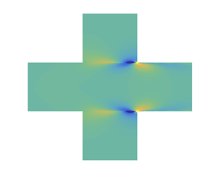
Figure 7. Spatial distribution of (a)  $\mathrm {Re}(\,p)$ and (b)
  $\mathrm {Re}(v)$ of the antisymmetric acoustic resonant mode at a real-valued frequency
  $\omega _A=0.3673$ (a trapped mode). (c) Variation of
  $p$ (red) and
  $v$ (blue) along
  $y$ at
  $x=L/2$. Dashed lines,
  $\mathrm {Re}(\,p)$ and
  $\mathrm {Re}(\textit {v})$; solid lines,
  $|p|$ and
  $|v|$. (d) Wavenumbers of the travelling waves. (e) Mode coefficients of the travelling waves in the
  $+x$ direction, where the modes are sorted according to their orders. The legend in (d) also applies to (e).

Figure 8. Spatial distribution of (a)  $\mathrm {Re}(\,p)$ and (b)
  $\mathrm {Re}(v)$ of the symmetric acoustic resonant mode at a complex frequency
  $\omega _A=0.3885 + 0.1350\mathrm {i}$. For the descriptions of (c–e), see figure 7.
The antisymmetric acoustic resonant mode displayed in figure 7(a–c) is a trapped mode. The coefficients of the  $+x$ travelling modes in the cavity segment (at
  $x=0$) and in the right duct (at
  $x=L$) are shown in figure 7(e), where the travelling modes have been normalized so that
  $|P_n(y)|_{{max}} = 1$. Note that the coefficient of the
  $n$th
$n$th  $-x$ travelling mode in the cavity segment (at
  $x=L$) or in the left duct (at
  $x=0$), which is not shown, is exactly the same as that of the
  $n$th
$n$th  $+x$ travelling mode. The split between symmetric and antisymmetric travelling modes in such a symmetric system can be seen: compared with the antisymmetric counterparts, the symmetric travelling modes have vanishingly small amplitudes. The zero amplitude of the outgoing propagative (cut-on) mode in each duct, as indicated numerically in figure 7(e) by the vanishingly small mode coefficient of the
  $n=1$ mode in the duct, means that acoustic energy of the trapped mode cannot escape, and consequently the trapped mode occurs at a real-valued frequency. Such a wave trapping mechanism in a symmetric system, i.e. because of symmetric mismatch, the antisymmetric trapped mode is decoupled from the outgoing plane waves in the two semi-infinite ducts which are the only cut-on modes in the ducts at the trapped mode frequency, has been extensively studied (Evans & Linton Reference Evans and Linton1991; Evans, Levitin & Vassiliev Reference Evans, Levitin and Vassiliev1994; Evans & Porter Reference Evans and Porter1997; Pagneux Reference Pagneux2013). The symmetric acoustic resonant mode, shown in figure 8(a–c), is assembled by symmetric travelling modes. The non-vanishing amplitude of the outgoing propagative mode in each duct, as shown in figure 8(e), means radiation of acoustic energy to infinity, thus the resonant mode is damped. Owing to the outgoing propagative modes in the ducts,
  $|k_{fl}|<1$ if the frequency remains real valued. To satisfy the feedback-loop closure principle for a resonant mode (
 $k_{fl}=1$),
  $\mathrm {Im}(\omega )$ increases. As shown in figure 8(d), for the two
  $+x$ propagative modes in the cavity segment
  $\mathrm {Im}(k)>0$, since
  $\mathrm {Im}(\omega _A)>0$.
The acoustic resonance frequency of the configuration can be approximately estimated with a one-dimensional model, assuming a resonance happens when  $\lambda /2=H+2D$ or
  $\lambda /4=D$, where
  $\lambda$ is the wavelength. However, the two resonant modes shown in figures 7 and 8 are close to but not exactly the same as the
  $\lambda /2$-resonance between the two cavity bottoms (see figure 7c) or the
  $\lambda /4$-resonance in each cavity (see figures 7c and 8c). The
  $\lambda /2$- and
  $\lambda /4$-resonance frequencies are
  $\omega _{\lambda /2}=0.3491$ and
  $\omega _{\lambda /4}=0.3927$. In the present case,
  $\omega _{\lambda /2}<\omega _{A,anti}<\mathrm {Re}(\omega _{A,sym})<\omega _{\lambda /4}$. The discrepancies in frequency depend on the geometrical parameters, and in general they reduce as the cavity depth is increased (Koch Reference Koch2005; Hein et al. Reference Hein, Koch and Nannen2012). It is noted here that for
  $D/L=1$ in § 3.1, the lowest acoustic resonance frequency is
  $\omega _{A,anti}=1.9387$ when
  $R=0$, which is much higher than the frequency range considered there.
For a comparison later in § 3.3, the acoustic resonant modes for the configuration  $D/L=8$ without flow but with a resistive sheet
  $R=0.018$ added at the entrance of each cavity are also calculated here. The complex frequencies of the first antisymmetric and symmetric resonant modes are respectively
  $\omega _A=0.3761 + 0.0044\mathrm {i}$ and
  $\omega _A=0.3881 + 0.1415\mathrm {i}$, which indicate that the influence of the small
  $R$ on
  $\mathrm {Re}(\omega _A)$ is extremely small and
  $\mathrm {Im}(\omega _A)$ is only slightly increased owing to the damping effect of
  $R$. Note that since the symmetry holds after the resistive sheets are introduced, the antisymmetric resonant mode, a lightly damped mode, however, is still a trapped mode (the outgoing propagative mode in each duct still has a zero amplitude).
The resonant modes presented in figures 7 and 8 are eigensolutions without forcing. As an acoustic forcing is introduced from the left duct, the wave scattering of the resonator is shown in figure 9, which is used to further discuss the purely acoustic resonances in figures 7 and 8 where  $R=0$, and to provide the forced acoustic fields inside the deep cavities at and far from the acoustic resonance frequencies that will be compared with the global modes in § 3.3 where
  $R \neq 0$. The calculation of wave scattering based on the scattering matrix method has been described in Dai & Aurégan (Reference Dai and Aurégan2018) and Dai (Reference Dai2020). The plane-wave transmission and reflection coefficients of the resonator are plotted in figure 9(a), which shows a zero transmission caused by the symmetric resonant mode. As the difference between the incident frequency and the resonant mode frequency is increased, the amplitude of the excited oscillations in the resonator decreases, as shown in figure 9(d–f). The antisymmetric resonant mode cannot be excited by an incoming plane wave owing to symmetric mismatch, thus its effect is not seen in figure 9(a). In figure 9(b,c), the resonator is excited by the first
  $+x$ cross-mode in the left duct. At the frequency of the antisymmetric resonant mode, the forcing excites a stronger oscillation in the resonator compared with figure 9(d–f), since the antisymmetric resonance has a larger quality factor. Note that, when
  $R=0$, the quality factor of such a perfect resonance is infinity and the amplitude of response is also infinity. The present numerics indicate the pressure amplitude at the cavity bottoms shown in figure 9(b) to be
  $|p|=1.15 \times 10^8$ if
  $R=0$. In figure 9 and § 3.3, the pressure is shown in
  $|p|$ rather than
  $\mathrm {Re}(\,p)$ for a better visual comparison (see the acoustic pressure nodes inside the deep cavities in figures 9(e,f) and 14(d,e)). At
  $y=0$,
  $|p|=0$ and
  $|p|\neq 0$ respectively indicate antisymmetric and symmetric resonant modes.

Figure 9. (a) Transmission and reflection coefficients for a plane-wave excitation (thin lines:  $R=0$, thick lines:
  $R=0.018$). (b,c) Value of
  $|p|$ excited by the first
  $+x$ cross-mode in the left duct of amplitude
  $|p|_{{max}}=1$ at
  $x=0$, at frequencies denoted by red vertical lines in (a):
  $\omega =\mathrm {Re}(\omega _A)$ where
  $\omega _A=0.3761 + 0.0044\mathrm {i}$ (antisymmetric acoustic resonance) and
  $\omega =0.3949$ (frequency in figure 12e). (d–f) Value of
  $|p|$ excited by the
  $+x$ plane wave in the left duct of amplitude
  $|p|=1$, at frequencies denoted by blue vertical lines in (a):
  $\omega =\mathrm {Re}(\omega _A)$ where
  $\omega _A=0.3881 + 0.1415\mathrm {i}$ (symmetric acoustic resonance),
  $\omega =0.5476$ (frequency in figure 14d) and
  $\omega =0.7708$ (acoustic anti-resonance). In (b–f),
  $R=0.018$.
3.3. Vortical–acoustic resonance in an AR
The problem sketched in figure 1(b) is discussed in this subsection. At low Mach numbers, the  $\textrm {KH}+\textrm {RPR}$ feedback loop occurring at the junction between the flow duct and the deep cavities is still acoustically compact, but this compact region is influenced by the acoustics of the resonator (Peters Reference Peters1993; Kriesels et al. Reference Kriesels, Peters, Hirschberg, Wijnands, Iafrati, Riccardi, Piva and Bruggeman1995).
The global mode frequency as a function of the Mach number is plotted in figure 10. At  $M_0=0.03$, the global mode frequency for
  $D/L=8$, being very close to those for
  $D/L=1$, approximately agrees with the Strouhal law. As
  $M_0$ increases,
  $\mathrm {Re}(\omega _G)$ of the antisymmetric mode progressively deviates from the Strouhal law, and the deviation becomes more noticeable as
  $\mathrm {Re}(\omega _G)$ gets close to the frequency of the antisymmetric acoustic resonant mode,
  $\mathrm {Re}(\omega _A)$. The temporal growth rate,
  $-\mathrm {Im}(\omega _G)$, shows a global mode destabilization when
  $\mathrm {Re}(\omega _G)$ is around
  $\mathrm {Re}(\omega _A)$, and a maximum temporal growth rate occurs when
  $\mathrm {Re}(\omega _G)= \mathrm {Re}(\omega _A)$ (Yamouni et al. Reference Yamouni, Sipp and Jacquin2013), which in this case happens at
  $M_0 \approx 0.09$. Note that the acoustic resonance frequency might be slightly shifted owing to the convection of the acoustic waves by the flow. This shift, however, should be extremely small since the flow speed is low, thus the maximum temporal growth rate happens when
  $\mathrm {Re}(\omega _G)$ equals to the
  $\mathrm {Re}(\omega _A)$ calculated without flow. For the symmetric modes, the influence of the heavily damped acoustic resonant mode on the global modes is rather weak near the frequency crossing point. The deviation of
  $\mathrm {Re}(\omega _G)$ from the Strouhal law is small. However,
  $\mathrm {Im}(\omega _G)$ shows a stabilization phenomenon over a
  $M_0$ range where
  $\mathrm {Re}(\omega _G)$ is much larger than
  $\mathrm {Re}(\omega _A)$. It is noted that, in the grey region in figure 10(b) (also in figure 15),
  $\mathrm {Im}(\omega _G)$ is high. For example,
  $\omega _G = 0.5213 + 0.0843 \mathrm {i}$ when
  $M_0=0.11$. We do not try to find the
  $M_0$ at which a peak
  $\mathrm {Im}(\omega _G)$ occurs, but mark that region in grey.

Figure 10. Global mode frequency  $\omega _G$ as a function of
  $M_0$: comparison between the deep-cavity case (
 $D/L=8$) and the shallow-cavity case (
 $D/L=1$). In (a),
  $\omega _A$ of acoustic resonant modes (
 $0.3671 + 0.0044\mathrm {i}$ and
  $0.3881 + 0.1415\mathrm {i}$) are calculated with
  $R=0.018$ without flow. The legend in (a) also applies to (b).
The different  $\mathrm {Im}(\omega _G)$ trajectories of the antisymmetric and symmetric global modes explain the previous experiments, from a linear point of view, that vortex structures are not shed simultaneously from the upper and lower cavity leading edges but with a shift of half a period (Peters Reference Peters1993; Kriesels et al. Reference Kriesels, Peters, Hirschberg, Wijnands, Iafrati, Riccardi, Piva and Bruggeman1995; Oshkai & Yan Reference Oshkai and Yan2008; Wang, Deng & Liu Reference Wang, Deng and Liu2018). Note that both antisymmetric and symmetric global modes could be unstable near the crossing point of
  $\mathrm {Re}(\omega _G)$ and
  $\mathrm {Re}(\omega _A)$ if the shear layer thickness is reduced, but the antisymmetric one should win in the competition owing to its larger temporal growth rate.
To explain the different  $\omega _G$ trajectories of the antisymmetric and symmetric global modes in figure 10, we adopt the view sketched in figure 11 that the vortical–acoustic resonance in an acoustic resonator and the associated system instability are governed by the KH instability waves and dual feedbacks: the RPR and AR feedbacks (Powell Reference Powell1990; Fabre & Hirschberg Reference Fabre and Hirschberg2000; Rienstra & Hirschberg Reference Rienstra and Hirschberg2018).

Figure 11. Vortical–acoustic resonance in an AR: KH instability and dual feedbacks. Adapted from Rienstra & Hirschberg (Reference Rienstra and Hirschberg2018).
The spatial distributions of the antisymmetric (figures 12 and 13) and symmetric (figure 14) global modes are plotted for different  $M_0$, where the fields have been normalized by
  $v$ at
  $x=L/4$ and
  $y=-H/2$. Figures 12(a,f) and 14(a,f) show that, when
  $\mathrm {Re}(\omega _G)$ is much lower than
  $\mathrm {Re}(\omega _A)$, at a very low Mach number
  $M_0=0.03$, the acoustic effect of the resonator barely shows in the spatial distributions, i.e. the whole resonator is compact. As
  $\mathrm {Re}(\omega _G)$ increases with the increasing
  $M_0$, the acoustic effect of the resonator on the
  $|p|$ distribution progressively appears. Note in figure 10(a) that, for global and acoustic resonant modes of the same symmetry,
  $\mathrm {Re}(\omega _G)$ only coincides with
  $\mathrm {Re}(\omega _A)$ at one particular value of
  $M_0$ as
  $\mathrm {Re}(\omega _G)$ varies continuously with
  $M_0$, since the antisymmetric or symmetric acoustic resonant mode only occurs at one discrete frequency in the frequency range considered. However, the influence of the resonator on the global modes appears over continuous Mach number and frequency ranges. It is also interesting to compare the
  $|p|$ distribution here with those shown in figure 9. The excitation frequencies in figures 9(c) and 9(e) respectively equal to
  $\mathrm {Re}(\omega _G)$ in figures 12(e) and 14(d). The resemblance in the
  $|p|$ distribution inside the cavities can be observed when the frequencies coincide, even though one is an externally excited field whereas the other is an eigenfunction describing the two-way excitation between vortical and acoustic motions in an AR.

Figure 12. Spatial distributions of the antisymmetric global modes for  $M_0=0.03$, 0.06, 0.09, 0.12 and 0.15 (rows 1 to 5). Column 1,
  $|p|$; column 2,
  $\mathrm {Re}(v)$; columns 3 and 4, amplitude and phase of
  $v$ along the opening of the low cavity (at the point just below
  $y=-H/2$). Blue lines, vortical; red lines,
  $-x$ acoustic; cyan lines,
  $+x$ acoustic; black lines, total (all travelling modes).

Figure 13. Spatial distributions of the antisymmetric global modes for  $M_0=0.0985$ (row 1,
  $\omega _G=0.3787 - 0.0175\mathrm {i}$) and
  $0.0990$ (row 2,
  $\omega _G=0.3792 - 0.0172\mathrm {i}$), between which the mode switching occurs. See figure 12 for the descriptions of the columns.

Figure 14. Spatial distributions of the symmetric global modes for  $M_0=0.03$, 0.06, 0.09, 0.12 and 0.15 (rows 1 to 5). See figure 12 for the descriptions of the columns.
Note that the different variation in  $|p|$ at the cavity bottoms with frequency shown in figures 12–14 from those in figure 9 might be due to the compressibility effect changing with
  $M_0$ and also the variation in global mode distribution (the global modes are normalized by
  $v$ at a constant position).
We now analyse the phase relation and the Strouhal number. The variations of  $v$ along the line between the upstream and downstream edges of the lower cavity are plotted in the third and fourth columns in figures 12–14. By observing those variations, one can analyse the effect of the AR on the
  $\textrm {KH}+\textrm {RPR}$ loop that mainly happens at the cavity openings. For the antisymmetric modes, figure 12(p,q,r,s,t) shows that the phase difference of the vortical disturbances between the edges reduces as
  $M_0$ is increased. Nevertheless, the phase difference of the
  $-x$ acoustic disturbances between the edges also changes with
  $M_0$, and the total phase variation around the feedback loop, which is approximately represented by the phase variation of the vortical disturbances from the upstream to the downstream edge plus the phase variation of the
  $-x$ acoustic disturbances from the downstream to the upstream edge, remains close to an integral multiple of
  $2{\rm \pi}$. For the symmetric modes, figure 14(p,q,r,s,t) shows that the variation of the phase difference of the vortical disturbances between the edges with the increasing
  $M_0$ is small. The phase variations are further displayed in figure 15(a,b), which shows that the variation of the phase difference of the KH waves between cavity edges is directly linked to the
  $-x$ acoustic disturbances, required by loop closure.

Figure 15. Phase difference (a,b) and amplitude ratio (c,d) of  $v$ at the upstream and downstream cavity edges (blue and red crosses,
  $\pm x$ disturbances; solid squares, the KH waves; circles, the phase change of
  $-x$ disturbances plus the phase change of
  $+x$ disturbances). (e,f) Wavenumbers of the KH waves (solid squares and diamonds,
  $\mathrm {Re}(k_{{KH}})$ and
  $\mathrm {Im}(k_{{KH}})$ calculated with
  $\omega _G$; hollow squares and diamonds,
  $\mathrm {Re}(k_{{KH}})$ and
  $\mathrm {Im}(k_{{KH}})$ calculated with
  $\mathrm {Re}(\omega _G)$). Rows 1 and 2: antisymmetric and symmetric global modes.
An interpretation of the variation of the KH phase difference between the upstream and downstream edges in the antisymmetric and symmetric global modes, from the dual-feedback view, is as follows. In the antisymmetric global modes in figure 12, the acoustic resonant mode is a nearly perfect resonant mode with a high quality factor, as discussed in § 3.2. At frequencies near  $\mathrm {Re}(\omega _A)$, the AR feedback, having an amplitude much higher than that of the RPR feedback at the cavity leading edges, dominates in the total feedback. Thus, the quick variation of the KH phase difference near
  $\mathrm {Re}(\omega _A)$ is due to the quick phase change with frequency in the response function of the AR (Tonon et al. Reference Tonon, Golliard, Hirschberg and Ziada2011). On the other hand, the heavily damped symmetric acoustic resonant mode has a minor influence on the loop phase relation in figure 14, since the corresponding response function has a low magnitude and a slowly varying phase.
The Strouhal number defined as  $Sr=\mathrm {Re}(\omega _G)L/2{\rm \pi} M_0$ is reformed,
 \begin{equation} Sr=\frac{\mathrm{Re}(\omega_G)L}{2{\rm \pi} M_c} \frac{M_c}{M_0}, \end{equation}
where  $M_c$ is the convection velocity of the KH waves. The first term on the right-hand side of (3.1) equals the ratio between the cavity length and the KH wavelength, and equals the phase difference of the KH waves between cavity edges, i.e.
  $\Delta \phi _{KH}/ 2{\rm \pi} =L/\lambda _{KH}=\mathrm {Re}(\omega _G)L/2{\rm \pi} M_c$. Thus, the essential mechanism of the frequency deviation from the Strouhal law shown in figure 10(a), which reflects the deviation of
  $\Delta \phi _{KH}$ from
  $2{\rm \pi}$, is the upstream feedback being affected by the AR, or the coexistence of RPR and AR feedbacks. Note that for a parallel velocity profile,
  $M_c/M_0$ also depends on
  $Sr$ (Michalke Reference Michalke1965; Schmid & Henningson Reference Schmid and Henningson2001), and this relation also influences the finally selected frequency of a global mode.
It is shown in figure 10(a) that the reduction of the Strouhal number of the antisymmetric global modes continues even though  $M_0$ is no longer close to
  $M_0=0.09$. This might be linked to the global mode switching, that is, the total phase change around the feedback loop jumping from
  $2j{\rm \pi}$ to
  $2(\kern1.5pt j-1){\rm \pi}$, where
  $j$ is an integer. The mode switching is shown in figures 12(r,s) and 15(a). Here, the switching happens slightly later than the maximum temporal growth rate as
  $M_0$ is increased, which is in line with the result of Yamouni et al. (Reference Yamouni, Sipp and Jacquin2013). The switching is found to occur suddenly during the increase of
  $M_0$. Figure 13 elaborates the mode switching and shows that the switching is linked to the
  $-x$ acoustic disturbances. The
  $\pm {\rm \pi}$ phase jump and the zero amplitude suggest that
  $v$ of the
  $-x$ acoustic disturbances changes sign between the downstream and upstream edges. Such a phenomenon, not happening in the compact case, indicates the interaction between the RPR and AR feedbacks here. Note that the phase jump can only be observed near the entrance of the cavities (
 $y=\pm H/2$) where both the
  $\textrm {KH}+\textrm {RPR}$ loop and the additional AR feedback are at play. At positions inside the deep cavities, the disturbance field, almost completely governed by the AR, is uniform in the
  $x$ direction. The phase jump happening in the
  $-x$ acoustic disturbances rather than in the KH wave also suggests that the mode switching is not a vortical but an acoustic effect.
The present linear global mode analysis for the compact and deep-cavity cases might also provide some insight into the frequency lock-in phenomenon in experiments. In the compact case, since the phase difference of the KH waves between the edges is almost constant and approximately equals to  $2{\rm \pi}$, owing to the fact that the solo RPR feedback is nearly hydrodynamic, the oscillation frequency roughly follows the Strouhal law. When an AR is involved, the total feedback is affected by the additional AR feedback, thus
  $\Delta \phi _{KH}/ 2{\rm \pi}$ accordingly changes to satisfy the loop phase relation. Moreover,
  $\Delta \phi _{KH}/ 2{\rm \pi}$ varies quickly with frequency when
  $\mathrm {Re}(\omega _G)$ is near the
  $\mathrm {Re}(\omega _A)$ of an acoustic resonant mode which has a small
  $\mathrm {Im}(\omega _A)$. Such a linear mechanism of frequency deviation from the Strouhal law is described in this work. It is noted that a linear mode-coupling mechanism has also been discussed for the frequency lock-in in vortex-induced vibrations (de Langre Reference de Langre2006). The measured frequency of self-sustained cavity flow oscillations also depends on the oscillation amplitude which affects the convection velocity of the vortical motions (
 $M_c/M_0$). At high amplitudes, the shear layer, strongly perturbed by the intense feedback acoustic waves at the separation point, rolls up into concentrated vortex structures (Ho & Huerre Reference Ho and Huerre1984). A minimum value of
  $M_c/M_0$ happens at the Mach number of maximum oscillation amplitude (Ma et al. Reference Ma, Slaboch and Morris2009). In some cases, clear vortex structures may not be observed, but the shear layer can be thickened by medium amplitude oscillations, which also leads to a decrease of the convection velocity (Boujo, Bauerheim & Noiray Reference Boujo, Bauerheim and Noiray2018).
The coexistence of the RPR and AR feedbacks also explains the stabilization and destabilization shown in figure 10(b). As shown in the compact case in § 3.1, the amplitude of the RPR feedback disturbances is very small at the upstream separation points. For the antisymmetric modes in the deep-cavity case, the AR feedback is strong near the frequency of the acoustic resonant mode. Thus, compared with the solo RPR feedback, the amplitude of  $-x$ acoustic disturbances at the leading edges is increased in the deep-cavity case, which decreases the ratio between the amplitudes of the
  $-x$ feedback disturbances at
  $x=L$ and at
  $x=0$. For the symmetric modes, the weak AR feedback at the upstream edge may have a comparable amplitude as the RPR feedback but an opposite phase. Those two feedbacks then cancel each other at the upstream edge, which leads to an extremely large ratio between the amplitudes of the
  $-x$ feedback disturbances at
  $x=L$ and at
  $x=0$. To satisfy the amplitude relation of the feedback loop for a global mode, the imaginary part of the frequency should be adjusted (see discussion in figure 6). The above analysis is clearly confirmed in figure 15(d) for the symmetric global modes, even though the plot only approximately represents
  $\boldsymbol{\mathsf{P}}_{u}$ and
  $\boldsymbol{\mathsf{P}}_{d}$ of the feedback loop. It demonstrates the large ratio between
  $|v|$ at the downstream edge and
  $|v|$ at the upstream edge, for the
  $-x$ feedback disturbances owing to the mutual cancellation between RPR and AR feedbacks at the upstream edge and also for the symmetric KH mode owing to the amplitude requirement for loop closure. The large
  $\mathrm {Im}(k_{\mathrm {KH}})$ indicated in figure 15(d) is linked to the increase of
  $\mathrm {Im}(\omega _G)$ (stabilization), as shown in figure 15(f). For the antisymmetric global modes,
  $|v|$ ratios for the
  $-x$ feedback disturbances and for the KH wave do not show the same trend, as shown in figure 15(c), which seems due to the global mode switching. A simple and intuitive demonstration of the feedback-loop destabilization is not obtained at this moment, although figure 15(e) shows the reduction of
  $\mathrm {Im}(k_{\mathrm {KH}})$ over the
  $M_0$ range of destabilization.
4. Conclusion
Vortical–acoustic resonance in 2-D symmetric duct–cavity configurations is studied by a linear global mode analysis about a low-speed inviscid parallel shear flow. In practice, even in the linear regime, the shear layer over a cavity develops, thus both convection velocity and spatial growth rate of vortical disturbances vary across the cavity. Because of the longitudinal-homogeneity and inviscid-flow assumptions and the added resistance in the calculations, the present results are of qualitative interest only. Nevertheless, such a mean flow model renders a neat separation of vortical and acoustic disturbances and a combined travelling–global mode analysis, which offer insight into some essential mechanisms involved.
First, in a shallow-cavity case, results are in line with the previous understanding of the Rossiter modes in compact cases. Vortical–acoustic resonance and the associated global instability, owing to the KH instability and the RPR feedback, can be supported by an incompressible model, where the feedback disturbances are purely hydrodynamic. The difference between incompressible and compressible models in describing the compact  $\textrm {KH}+\textrm {RPR}$ feedback loop at low flow speeds is small. The phase difference of the unstable vortical waves between the upstream and downstream cavity edges is close to
  $2{\rm \pi}$, i.e.
  $\Delta \phi _{KH}/ 2{\rm \pi} \approx 1$, and the global mode frequency agrees with the Strouhal law.
The influence of an AR on the  $\textrm {KH}+\textrm {RPR}$ feedback loop is then examined. Note that, for symmetric configurations, the split between antisymmetric and symmetric travelling modes occurs in both acoustic and vortical–acoustic resonant modes. In this deep-cavity case, two acoustic resonant modes occur in the frequency range considered: the antisymmetric one is a trapped mode (lightly damped by the resistive sheets introduced in the calculations) whereas the symmetric one is a heavily damped mode due to radiation. As the Mach number is increased, different trajectories of the antisymmetric and symmetric global modes are observed. The frequency of the antisymmetric global modes deviates from the Strouhal law and the global modes are destabilized when the global mode frequency is close to the frequency of the antisymmetric acoustic resonant mode. A global mode switching is also observed. On the other hand, the influence of the symmetric acoustic resonant mode on the global modes is much smaller. Nevertheless, a stabilization of the symmetric global modes is observed. We have shown that the global mode-related phenomena can be explained by the local–global relation of the feedback loop and the dual-feedback view: the coexistence of the RPR and AR feedbacks. The frequency deviation from the Strouhal law is due to
  $\Delta \phi _{KH}/ 2{\rm \pi}$ being changed by the additional AR feedback, and
  $\Delta \phi _{KH}/ 2{\rm \pi}$ changes quickly with frequency when the global mode frequency is near the frequency of an acoustic resonant mode with a high quality factor, such as a trapped mode. Such a linear result provides some insight into the frequency lock-in phenomenon in experiments, although the frequency of self-sustained cavity flow oscillations also depends on the oscillation amplitude. It is found that the global mode switching is not a vortical but an acoustic effect. The switching results from the interaction between the RPR and AR feedbacks, whereas the vortical motions do not show signs of the sudden switching. The global mode destabilization and stabilization are respectively understood as the result of the total feedback at the upstream edge being strengthened and weakened by the additional AR feedback.
Funding
This work has been supported by the National Natural Science Foundation of China no. 51876120.
Declaration of interests
The author reports no conflict of interest.
Appendix A. Convergence of calculations
The convergence of the present numerical calculations is assessed on table 1, using two global modes for  $D/L=8$ for example: GM1, the antisymmetric mode at
  $M_0=0.09$; GM2, the symmetric mode at
  $M_0=0.12$.
Table 1. Convergence assessment of the numerical calculations.

Appendix B. Multiple feedback-loop channels
Since in each system resonant mode there are multiple downstream- and upstream- travelling modes in the cavity segment, the feedback loop can be seen as the sum of multiple channels, each of which is associated with one downstream-travelling mode, one upstream-travelling mode and their mutual reflection at the segment ends. A preliminary analysis of the multiple feedback-loop channels is performed in figure 16 for the antisymmetric global modes of the compact and deep-cavity configurations. The wavenumbers in figure 16(a,b) show that the decay rates of several  $-x$ acoustic modes are less than or comparable to the growth rates of the KH modes, thus all those
  $-x$ acoustic modes are possible candidates for closing the loop, from the loop-gain consideration.

Figure 16. Multiple feedback-loop channel analysis of two antisymmetric global modes (row 1, figure 2(a,c),  $D/L=1$ and
  $M_0=0.9$; row 2, figure 12(c,h),
  $D/L=8$ and
  $M_0=0.9$). (a,b) Wavenumbers in the cavity segment, (c,d) mode coefficients of the KH and
  $\pm x$ acoustic modes in the cavity segment (triangles, KH; diamonds,
  $+x$ acoustic; squares,
  $-x$ acoustic. Solid and hollow symbols respectively denote the coefficients at the segment ends where the wave travelling starts and terminates), (e,f) Loop gain of each channel consisting of the antisymmetric KH mode and a
  $-x$ acoustic mode.
In the antisymmetric Rossiter mode of the compact case, the  $\pm x$ acoustic plane waves are not involved in the feedback loop owing to symmetric mismatch, as indicated by their vanishingly small coefficients in figure 16(c), thus the
  $-x$ acoustic modes closing the loop are all evanescent modes, among which the least attenuated mode has the highest amplitude at the upstream end. To examine the error of using a KH mode plus some less attenuated
  $-x$ acoustic modes to represent the Rossiter mode, the channel gain is calculated. Assuming that the
  $m$th element in
  $\boldsymbol {C}_{fl}$ is the coefficient of the antisymmetric KH mode, the loop gain of the channel consisting of the KH mode and the
  $n$th
$n$th  $-x$ acoustic mode is
  $G_{KH,n}=|\boldsymbol{\mathsf{M}}_{u}(m,n) \times \boldsymbol{\mathsf{M}}_{d}(n,m)|$, where
  $\boldsymbol{\mathsf{M}}_{u}=\boldsymbol{\mathsf{R}}_{u}\boldsymbol{\mathsf{P}}_{u}$,
  $\boldsymbol{\mathsf{M}}_{d}=\boldsymbol{\mathsf{R}}_{d}\boldsymbol{\mathsf{P}}_{d}$,
  $m$ and
  $n$ denotes the positions of the elements in the matrices. The result of
  $G_{KH,n}$ is plotted in 16(e), which shows that the first antisymmetric channel has the largest gain 0.817. The sum of the gains of
  $N_2$ channels is
  $G_{KH}=|\sum _{n} \boldsymbol{\mathsf{M}}_{u}(m,n) \times \boldsymbol{\mathsf{M}}_{d}(n,m)| = |\boldsymbol{\mathsf{M}}_{fl}(m,m)|=0.915$, which is close to but less than unity, denoting an amplitude variation of the KH mode after the loop through the
  $N_2$ acoustic channels. This indicates the effect of the other
  $+x$ travelling modes on the replication of the KH mode around a feedback loop. For the global mode in the deep-cavity case,
  $G_{KH}=0.292$. The global mode is now governed by the
  $\textrm {KH}+\textrm {RPR}$ loop, which may still be approximately described by a KH mode plus some less attenuated
  $-x$ acoustic modes, and the additional AR effect. In the travelling-mode representation of the latter, some
  $+x$ acoustic modes are as significant as their
  $-x$ counterparts, as indicated by the pressure distributions inside the deep cavities in §§ 3.2 and 3.3. Nevertheless, at the cavity openings (
 $y=\pm H/2$),
  $|v|$ associated with the group of the
  $+x$ acoustic modes is negligibly small compared with those of the vortical and the
  $-x$ acoustic groups (see column 3 in figures 12–14), which simplifies the downstream–upstream analysis of the feedback loop done in § 3.3.


