


1. Introduction
Capillary-gravity waves appear on the surface of a liquid and exhibit a dispersion relationship with a continuous spectrum, reflecting a balance between the liquid inertia and restorative forces of surface tension and gravity (Lamb Reference Lamb1932). When constrained by a finite-size tank, these waves tend to conform to the container geometry and exhibit a discrete spectrum described by an integer-valued mode number pair (Case & Parkinson Reference Case and Parkinson1957; Mei & Liu Reference Mei and Liu1973). Mechanically excited waves can be formed in experiment by vertically oscillating a tank filled with liquid having a meniscus pinned at the tank edge, thereby creating a travelling wave that propagates inward in the radial direction. These are referred to as edge waves and have frequency equal to that of the driving frequency, i.e. they are harmonic, as long as the forcing amplitude is below the Faraday wave threshold (Faraday Reference Faraday1831; Benjamin & Ursell Reference Benjamin and Ursell1954). When the container has a circular geometry, the waves propagate radially inward and reflect back out at the centre of the tank, causing wave interference. Resonance occurs when the driving frequency is equal to one of the resonance frequencies, in which case these waves interact constructively and form a standing wave described by the number of fixed circular nodes. Off resonance, the wave amplitude decreases, but is finite, and is characterised by its frequency-response diagram. In this paper, we are interested in the frequency response of circular edge waves in viscoelastic materials.
Bioprinting technologies exploit surface-wave patterns to assemble organoid cells (Chen et al. Reference Chen, Güven, Usta, Yarmush and Demirci2015) for tissue engineering applications (Guven et al. Reference Guven, Chen, Inci, Tasoglu, Erkmen and Demirci2015). In these technologies, the working material is often a soft gel (polymeric fluid), such as agarose or alginate, which is capable of sustaining biological function (Murphy & Atala Reference Murphy and Atala2014; Fan et al. Reference Fan, Piou, Darling, Cormier, Sun and Wan2016). Accordingly, it is important to understand the surface-wave dynamics on such materials in order to advance these technologies. Our work directly addresses this point and we report the first, to the best of the authors’ knowledge, experimental observation of edge waves in soft gels. A viscoelastic material exhibits both viscosity and elasticity, as defined by the complex modulus  $G'+iG''$ determined from rheological tests (Mezger Reference Mezger2006). Here
  $G'$ is the storage modulus and
  $G''$ the loss modulus, which describe the elasticity and viscosity, respectively, which often depend upon the frequency of applied shear. In our experiments, we select materials that exhibit constant rheological properties over the range of driving frequencies explored and whose rheological properties can be varied via concentration so that we can explore viscous and elastic effects independently over a wide range of properties. Specifically, we investigate (i) glycerol/water mixtures which give a range of viscosity
  $\mu$ at essentially zero elasticity and (ii) agarose gels whose gel concentration gives a range of shear modulus
  $G$ with relatively small viscosities, as illustrated in figure 1. Both materials are subject to surface-tension forces and this gives rise to two dimensionless numbers that define the viscoelastic properties (McKinley Reference McKinley2005), the Ohnesorge number
  ${Oh}\equiv \mu /\sqrt {\rho R \sigma }$ and elastocapillary number
  $\textrm {Ec}\equiv G R/\sigma$, where
  $R$ is the length scale. When
  ${Ec}\sim 1$, elastic forces and surface-tension forces are comparable and this belongs to the study of elastocapillarity (Style et al. Reference Style, Jagota, Hui and Dufresne2017; Bico, Reyssat & Roman Reference Bico, Reyssat and Roman2018). Agarose gel is a commonly used material for such studies because
  $G'$ is typically orders of magnitude larger than
  $G''$ meaning that elastocapillarity can be investigated largely independent of viscous effects (Grzelka, Bostwick & Daniels Reference Grzelka, Bostwick and Daniels2017; Shao et al. Reference Shao, Fredericks, Saylor and Bostwick2019, Reference Shao, Fredericks, Saylor and Bostwick2020). These are referred to as ‘inviscid elastic fluids’.

Figure 1. Illustration of viscoelastic behaviour of the materials explored in this investigation in the shear modulus  $G$ versus viscosity
  $\mu$ parameter space.
Edge waves are excited in experiment whenever the meniscus makes a contact-angle  $\alpha \neq 90^{\circ }$ and these are observed for small driving amplitude. At driving amplitudes larger than those explored here, sub-harmonic Faraday waves form, and these have been studied extensively for Newtonian liquids (Douady & Fauve Reference Douady and Fauve1988; Douady Reference Douady1990; Christiansen, Alstrøm & Levinsen Reference Christiansen, Alstrøm and Levinsen1992; Edwards & Fauve Reference Edwards and Fauve1994; Kumar & Bajaj Reference Kumar and Bajaj1995; Perlin & Schultz Reference Perlin and Schultz2000; Westra, Binks & Van De Water Reference Westra, Binks and Van De Water2003), though there are far fewer studies for complex fluids, perhaps because the presence of elasticity in gels is likely to lead to more complex behaviour.
Generally speaking, the motion of a liquid interface held by surface tension obeys an operator equation that resembles the damped-driven oscillator (DDO) (Bostwick & Steen Reference Bostwick and Steen2015),
 \begin{equation} \lambda^{2} M+\lambda D+K=A, \end{equation}
where  $\lambda$ is the scaled driving frequency,
  $A$ the driving amplitude,
  $M$ the liquid inertia operator,
  $D$ dissipation operator and
  $K$ the restorative force operator that encompasses capillarity. Viscous effects enter through
  $D$ and elastic effects through
  $K$. The presence of a meniscus can introduce dynamic wetting effects associated with a moving contact-line. Here a constitutive law is typically imposed that relates the dynamic contact-angle
  $\alpha$ to the contact-line speed
  $U_{CL}$,
  $\alpha =f(U_{CL})$ of which the pinned contact-line is a limiting case. Interestingly, dynamic wetting introduces contact-line dissipation, even for inviscid liquids, which was first realised by Davis (Reference Davis1980) and Hocking (Reference Hocking1987). This dissipation can be absorbed into the dissipation operator
  $D$ and its effects have been reported in the frequency response for driven sessile drops (Lyubimov, Lyubimova & Shklyaev Reference Lyubimov, Lyubimova and Shklyaev2006; Bostwick & Steen Reference Bostwick and Steen2016). The edge waves studied here have a pinned contact-line, i.e. no dynamic contact-line effects, such that the sole source of dissipation is due to viscosity.
With regard to edge waves in circular containers, Henderson & Miles (Reference Henderson and Miles1994) have theoretically investigated the case of a Stokes boundary layer with fixed contact-line with an interface that is either clean or contaminated with surfactant, and predicted the natural frequencies and damping ratios, which Martel, Nicolas & Vega (Reference Martel, Nicolas and Vega1998) have extended to include higher-order viscous effects. Kidambi (Reference Kidambi2009b) showed how the static contact angle affects the spectrum for a viscous liquid. With regard to moving contact-line modelling, Nicolás (Reference Nicolás2005) analysed the large Bond number limit for an inviscid fluid and has contrasted the case of free versus pinned contact-line and Kidambi (Reference Kidambi2009a) showed the existence of damping in an inviscid fluid owing to dynamic wetting effects. Recent work by Michel, Pétrélis & Fauve (Reference Michel, Pétrélis and Fauve2016) has shown the damping of surface waves by a meniscus. In our experiments, the contact-line is pinned and we develop a model for the natural frequencies of a viscoelastic material in a cylindrical container with a pinned contact-line. Several solution methods exist to address the pinned contact-line including a variational approach using a Lagrange multiplier (Benjamin & Scott Reference Benjamin and Scott1979; Graham-Eagle Reference Graham-Eagle1983), the introduction of a singular pressure at the contact-line (Prosperetti Reference Prosperetti2012), and a Rayleigh–Ritz minimisation procedure over a constrained function space (Bostwick & Steen Reference Bostwick and Steen2013a,Reference Bostwick and Steenb). We use the latter approach in our theoretical development.
Lastly, we mention the utility of using surface waves to distribute particulates (Wright & Saylor Reference Wright and Saylor2003; Saylor & Kinard Reference Saylor and Kinard2005), which can be extended to distributing cells in tissue engineering applications and surfactants (Strickland, Shearer & Daniels Reference Strickland, Shearer and Daniels2015) on thin liquid films. Picard & Davoust (Reference Picard and Davoust2007) have proposed using meniscus waves as a DNA biosensor, whereby the surface rheology is connected to biomolecules (Picard & Davoust Reference Picard and Davoust2006). Edge waves have also been used to measure liquid properties (Shmyrov et al. Reference Shmyrov, Mizev, Shmyrova and Mizeva2019) and surfactant properties (Saylor, Szeri & Foulks Reference Saylor, Szeri and Foulks2000). The flows associated with a meniscus can be complex as shown by Huang et al. (Reference Huang, Wolfe, Zhang and Zhong2020) for the case of a streaming flow.
We begin this paper by describing the experimental set-up and imaging techniques to quantify the magnitude of the wave field in § 2. Experimental results are reported in § 3 where we present frequency-response diagrams for our glycerol/water mixtures and agarose gels showing how viscosity and elasticity affect the resonance peaks and associated bandwidths. Complex resonance behaviours are reported for gels including a nonlinear side-band instability characterised by multiple resonance peaks for the same mode number. In § 4, we develop a theoretical model to predict the natural frequency and surface mode shapes of a viscoelastic fluid in a cylindrical container with a pinned contact-line. Comparisons between theoretical predictions and experimental observations are made and show good agreement. Lastly, we offer some concluding remarks in § 5.
2. Experiment
Edge waves were investigated using the experimental set-up shown in figure 2, which consists of a circular Plexiglas tank of radius  $R=35$ mm and depth
  $H=22$ mm mounted on a Labworks ET-139 electrodynamic shaker, which provides vertical vibration of the tank, controllable in amplitude and frequency. Experiments were conducted for a range of driving frequency
  $f_d=4.0\text {--}22.9$ Hz. The shaker is driven by an Agilent 33220A function generator, Labworks PA-141 amplifier combination. The acceleration of the shaker
  $A$ [
$A$ [ $\textrm {m}~\textrm {s}^{-2}$] was monitored using an PCB 352C33 accelerometer and a PCB 482C05 signal conditioner combination.
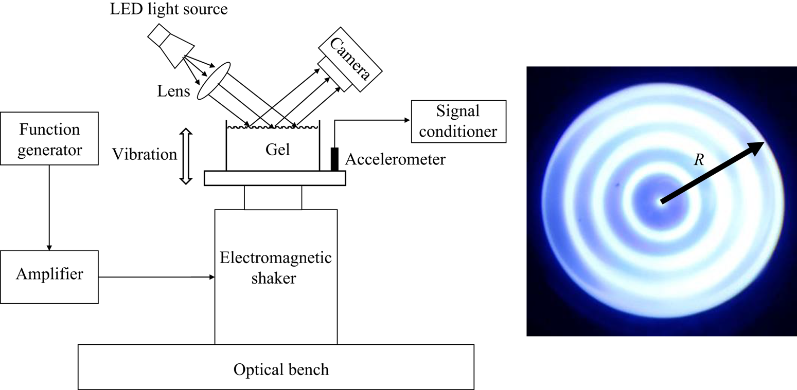
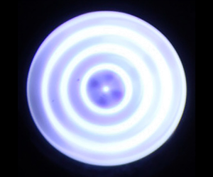
Figure 2. Schematic of the experimental set-up and a typical edge-wave pattern.
Glycerol/water mixtures and agarose gels were used to investigate the effect of viscosity and elasticity, respectively. These materials were chosen specifically for the ability to control the viscosity and shear modulus over a range of values, as discussed earlier. Doubly distilled water was used to prepare both the glycerol/water mixtures and agarose gels. One of the glycerol/water mixture cases was the limiting case of pure water. It is well known that adventitious surfactants can accumulate on pure water surfaces thereby affecting the surface tension. To avoid this we took care to use only doubly distilled water in all experiments, to clean out the tank after every experiment, and to limit the amount of time used to conduct an experiment. The material properties for the glycerol/water mixtures explored here are listed in table 1, where  $\mu$ is the viscosity,
  $\rho$ the density and
  $\sigma$ the surface tension (Takamura et al. Reference Takamura, Fischer and Morrow2012). The Ohnesorge number
  ${Oh}\equiv \mu /\sqrt {\rho R \sigma }$ is a measure of the relative importance of viscosity and surface tension and for our experiments
  ${Oh}=0.00064\text {--}0.0145$. The Bond number
  ${Bo}\equiv \rho g R^{2}/\sigma$ ranges from
  $\textrm {Bo}=170.8\text {--}223.7$. The agarose hydrogels used in our experiments were prepared by dissolving agarose powder (Sigma Aldrich, Type VI-A) in doubly distilled water at
  $90\,^{\circ }$C for an hour and then pouring the mixture into our circular Plexiglas tank, which was then allowed to gel at
  $25\,^{\circ }$C for 3 h. The concentration of the agarose solutions ranged from
  $\phi =0.061\text {--}0.125$ %w, which corresponds to a shear modulus
  $G=1.2\text {--}20.2$ Pa (Tokita & Hikichi Reference Tokita and Hikichi1987). The complex modulus
  $G'+i G''$ of the agarose gels was measured using a rheometer (Anton Paar, MCR 302). For the gels explored here, the storage modulus
  $G'$ is at least an order of magnitude larger than the loss modulus
  $G''$ implying that the gels used in our experiments essentially behave as inviscid elastic fluids with shear modulus
  $G$. The elastocapillary number
  ${Ec}\equiv G R/\sigma$ describes the relative importance of elastic to surface-tension forces. We note that extant methods for measuring surface tension could not be used because they would fracture the gel. Hence, we were prevented from measuring the actual surface tension of our gels. However, the gels used in experiment were made from very dilute concentrations of solutions and for this reason we assume the surface tension of our gels is
  $\sigma =72$ mN m
 $^{-1}$. This gives a range of
  ${Ec}=0.58\text {--}9.82$ used in these experiments.
Table 1. Material properties of glycerol/water mixtures, density  $\rho$, viscosity
  $\mu$, surface tension
  $\sigma$, taken from Takamura, Fischer & Morrow (Reference Takamura, Fischer and Morrow2012) and corresponding Ohnesorge
  ${Oh}$ and Bond
  ${Bo}$ numbers.

Our preliminary work revealed that edge waves are not formed when the fluid surface is perfectly flat, i.e.  $\alpha = 90^{\circ }$ (cf. Figure 3) and the best results were obtained when
  $\alpha < 90^{\circ }$, although
  $\alpha > 90^{\circ }$ is also sufficient. To ensure that this was the case and that we had a repeatable meniscus condition for all experiments, we filled the tank with a glycerol/water mixture or agarose solution so that the interface was pinned to the edge of the tank and was perfectly flat
  $\alpha =90^{\circ }$. Then, a pipette was used to carefully remove 2 ml of fluid giving a surface with
  $\alpha <90^{\circ }$. This ensures there are no dynamic wetting effects associated with a moving contact-line. For gels, the container was covered to prevent evaporation during gelation, after which experiments were conducted. We note that, though we work with a fixed value for
  $\alpha$ in this work, it is probably the case that wave amplitudes will vary with
  $\alpha$. Here we are only interested in generating edge waves and so any
  $\alpha$ not equal to 90
 $^{\circ }$ serves our purposes. Future studies addressing the effect of
  $\alpha$ on wave amplitude would be an interesting advancement of the present work.

Figure 3. Illustration of the meniscus and associated contact-angle  $\alpha$.
The wave pattern was characterised by the following procedure. A white-light source was collimated by a lens located one focal length  $f=300$ mm from the light source. To improve the degree of collimation, a plate with a 2 mm diameter hole was placed in front of the light source (a flashlight consisting of a white LED). This hole was located at the focal point of the lens providing a closer approximation to a point light source. The resulting collimated light beam was directed at the wave surface and the reflected light was captured by a digital camera (Canon EOS Rebel T3i, with a Canon EF-S 18–55 mm lens). The optical axis of the camera was oriented to coincide with the reflection of the collimated light beam. The camera exposure was set to 1s so that each image consisted of the integrated average of multiple wave periods, where only standing-wave modes produce a clear pattern and travelling-wave patterns are blurred. In this way, the wave field exhibits a high intensity in regions where the slope is zero (peaks and troughs) and a low intensity in regions where the wave slope is non-zero. Accordingly, the experimental images presented herein are wave-slope images where the intensity is inversely related to slope. This approach relies sensitively on the orientation of the camera optical axis with the spectral reflection of the collimated light from the flat surface and the degree of collimation of the light source. To ensure that these conditions were met, images of a flat surface were periodically acquired and checked to determine if a uniform image intensity is obtained. A typical image of such a check is shown in figure 4 which has an average intensity
  $I=250.5$ and an r.m.s. of
  ${\pm }4.46$ (
 ${\pm }1.8\,\%$). We note that in figure 4 and in subsequent figures, the intensity
  $I$ is the pixel intensity of the 8-bit images we acquired and hence varies from 0–255.

Figure 4. Reflection of the collimated light source as seen by the camera for a perfectly flat interface.
Frequency sweeps were performed and yielded a wave-slope image for each sampled frequency. The frequency increment was 0.5 Hz far from resonance and 0.2 Hz near resonance. A wait time of 5 seconds was imposed at each frequency before obtaining a wave-slope image in order to ensure a steady-state wave pattern. A typical experiment took 30 min. Figure 5(a) shows a sequence of wave-slope images as resonance is approached at  $f_d=16.9$ Hz. The resonance shapes for the
  $n=1\text {--}5$ modes are shown in figure 5(b) and we note the mode number
  $n$ corresponds to the number of dark rings in the image, i.e. nodes of the wave field, with the exception of the
  $n=4,5$ images, where the presence of the meniscus makes it difficult to fully resolve the nodes near the contact-line.
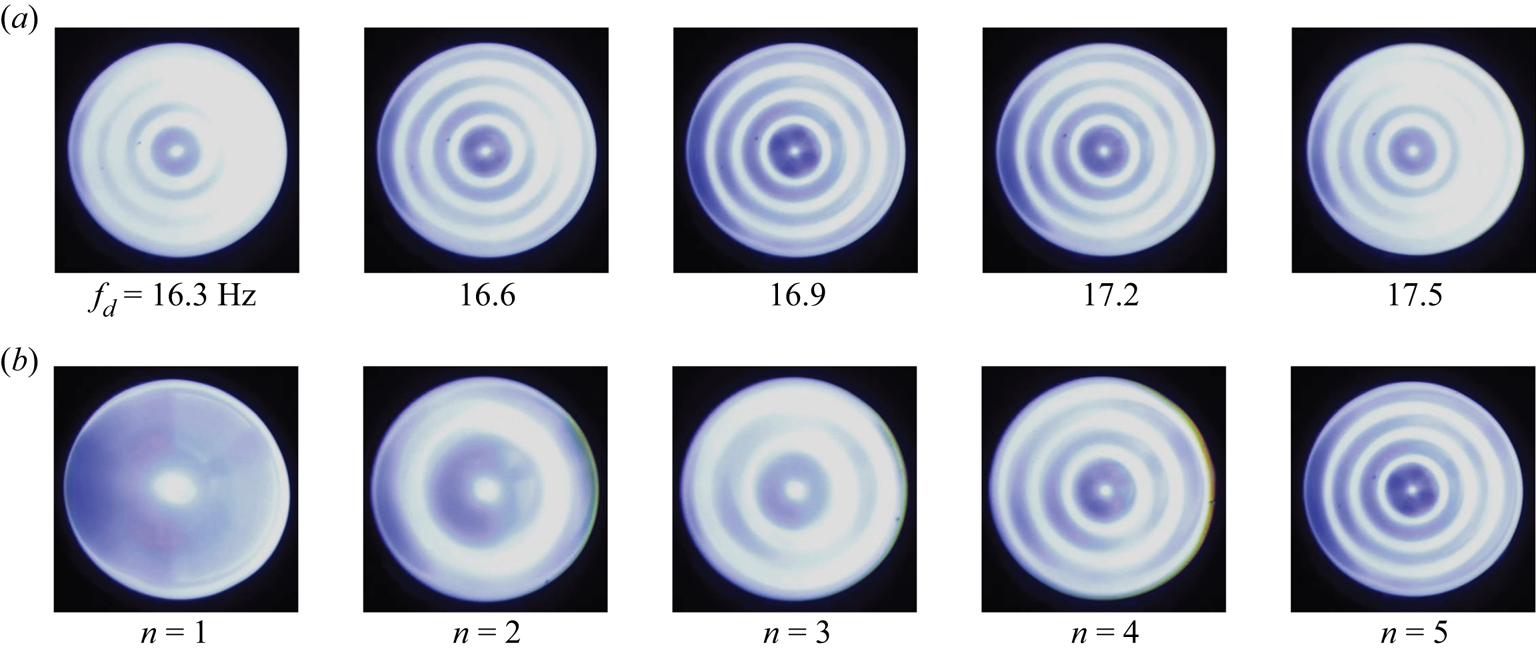
Figure 5. Wave-slope images for (a) driving frequencies  $f_d=16.3$ to 17.5 Hz show resonance is observed at
  $f_d=16.9$ Hz for the
  $n=5$ mode, as seen by the progressively less clear image as
  $f_d$ deviates from 16.9 Hz and (b) the associated resonance modes for
  $n=1,2,3,4,5$. The working material is water.
It is desirable to quantify the amplitude of the wave field and we do this using the wave-slope images. For each image, the light intensity  $I$ was azimuthally averaged and plotted against the radial coordinate
  $r$ to provide an intensity versus radius profile, an example of which is shown in figure 6. The maxima corresponds to locations of the peaks/troughs and the minima the nodes of the wave field. We use the quantity
  $E_{1}-E_{2}$ as a metric for the amplitude of the wave field, where
  $E_{1}$ and
  $E_{2}$ are the intensity at the first and second extrema in the
  $I$ versus
  $r$ plot (cf. figure 6). The intensity
  $E_{1}$ is that of a flat surface and will attain a maximum value at resonance which should differ little from the other peak intensities. This is supported by figure 6 which shows that all peaks have roughly the same intensity, of about 250. The intensity
  $E_2$ is the first node of the wave field and is the time-integrated average of the intensity observed by the camera as the wave slope oscillates between a peak-positive and peak-negative value. The difference
  $E_{1} - E_{2}$ is a good quantifier of the amplitude of the wave field because it should decrease away from resonance, where travelling-wave patterns average out over multiple wave periods to give an intensity field with lower maximum intensities and higher minimum intensities. At resonance, the peaks attain their maximum flat-surface value, while the nodes attain a minimum owing to the fact that the sloped surface is directing light away from the camera's optical axis for most of the wave period. Of course
  $E_{1} - E_{2}$ will also increase with the driving amplitude
  $A$, and since we wish to compare the intensity of the wave field at different frequencies without any sensitivity to the driving amplitude
  $A$, we characterise the magnitude of the wave field as
 \begin{equation} X=\frac{E_{1}/I_f-E_{2}/I_f}{A}.\end{equation}
This is an important point, as  $A$ varies with increasing frequency, given that we operate our amplifier in a constant voltage mode, resulting in an increase in
  $A$ with driving frequency. Scaling according to (2.1) ensures comparison of wave slopes on an equal acceleration basis. We note also that slight variations in the intensity of the light source and small day-to-day deviations of the geometric set-up of the camera and light source are possible and so we scale
  $E_{1}$ and
  $E_{2}$ to the average intensity of the most recent flat image
  $I_f$ (cf. figure 4). Frequency-response diagrams plotting
  $X$ against driving frequency
  $f_d$ are then obtained from which we can identify resonance frequency peaks, as will be discussed in the next section.
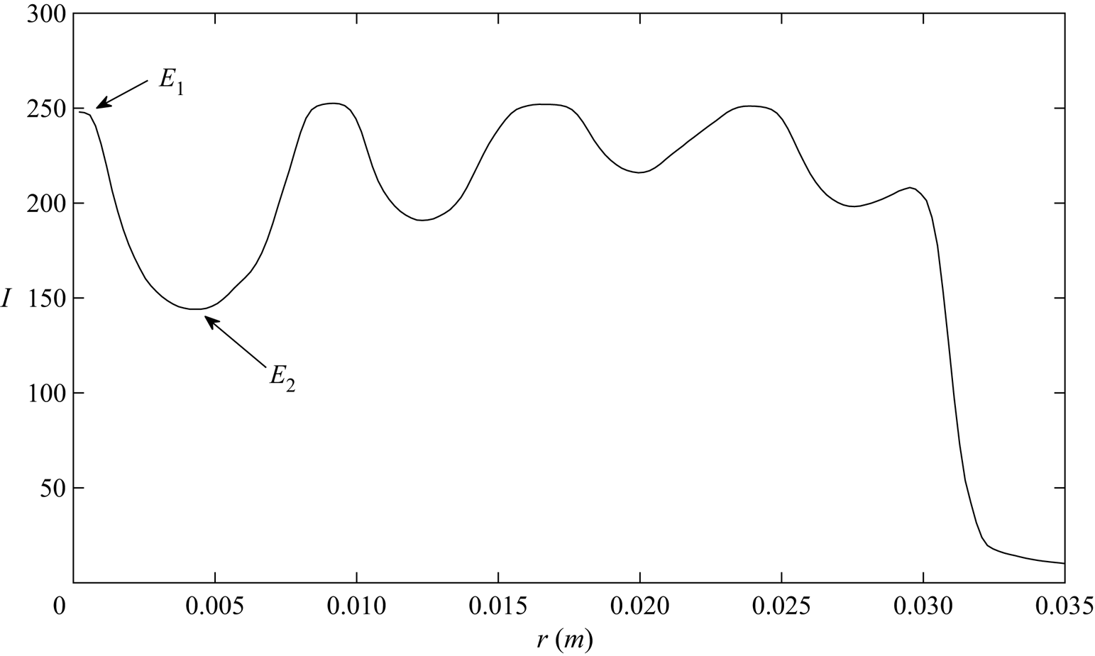
Figure 6. Azimuthally averaged light intensity  $I$ against radius
  $r$ show maxima and minima which correspond to locations of zero slope and zero displacement (large slope, nodes), respectively. The first two extrema
  $E_1$ and
  $E_2$ are the intensities of the first flat region and the first node with the difference
  $E_1$–
 $E_2$ used as a metric for the wave amplitude.
3. Experimental results
Frequency-response diagrams showing wave amplitude  $X$ against driving frequency
  $f_d$ are presented for a range of viscosity and elasticity. Each diagram shows a set of resonant peaks, each associated with a mode number
  $n$. Our focus is on how the resonance frequency and associated bandwidth are affected by viscosity and elasticity and how this depends upon the mode number
  $n$. In addition, we report multiple resonance peaks for a given mode
  $n$ that we associate with nonlinear wave–wave interactions typical of the Benjamin–Feir instability (BFI) (Benjamin Reference Benjamin1967; Benjamin & Feir Reference Benjamin and Feir1967).
3.1. Viscosity
Figure 7(a) is the frequency-response diagram for our glycerol/water mixtures and exhibits six resonance peaks for our least viscous liquid (water). A number of trends can be seen in the figure. First, increased viscosity leads to a smaller peak wave amplitude  $X$ and a larger bandwidth. Second, the bandwidth increases with mode number
  $n$ consistent with larger viscous dissipation for higher-mode numbers. Lastly, for fixed-mode number
  $n$ the resonance peak shifts to lower frequencies and the bandwidth increases with increasing viscosity, as illustrated in figure 7(b) for the
  $n=4$ mode. These observations are all consistent with the role of viscosity as the damping force in the classical DDO model. Surface tension plays the role of the restorative ‘spring’ force in the DDO. The aforementioned trends are all monotonic with viscosity
  $\mu$ and highlight this damping effect in the dynamics. It is also noted that as the viscosity is increased, the higher-frequency peaks begin to become overdamped and do not exhibit a well-defined resonance peak. For our most viscous liquid the modes
  $n=4,5,6$ cannot be discerned.
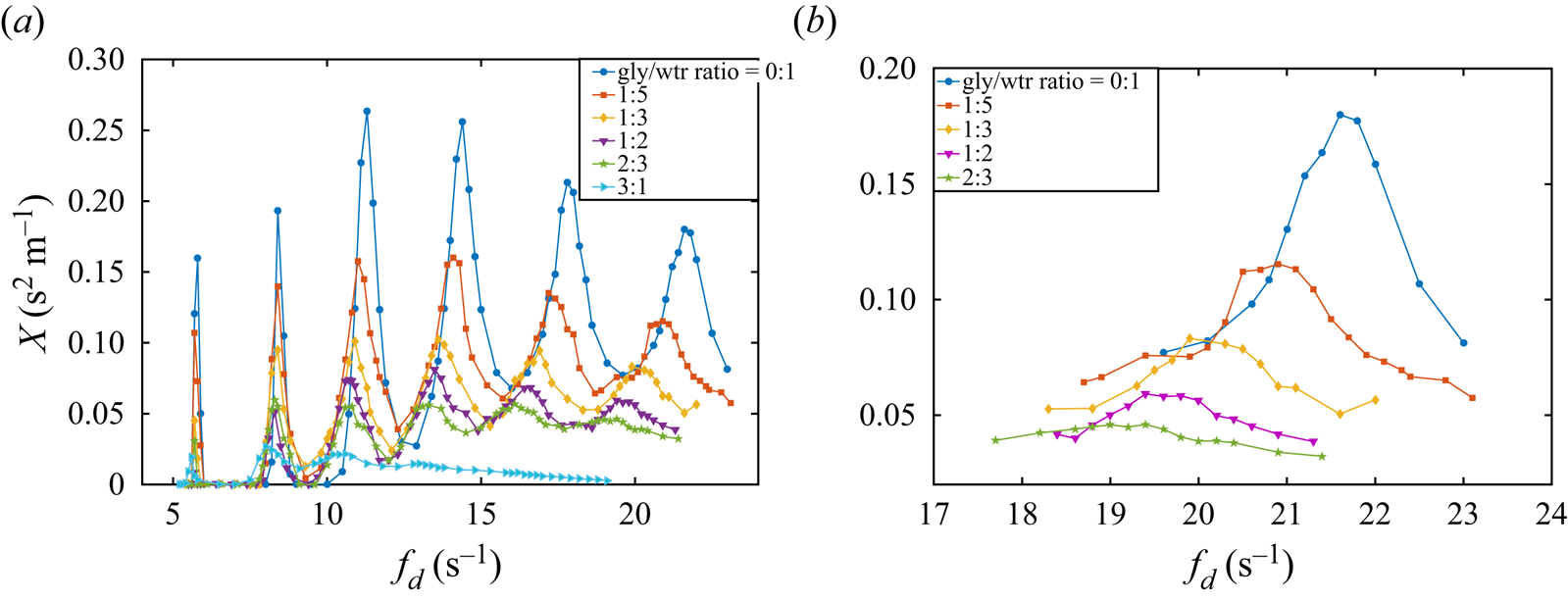
Figure 7. Frequency response, showing scaled amplitude  $X$ against driving frequency
  $f_d$ for (a) the full frequency range and (b) expanded view of the
  $n=4$ mode for glycerol/water mixtures with material properties listed in table 1.
3.2. Elasticity
Gels have finite elasticity, which we expect to act in a similar manner to surface tension thereby providing a more robust restoring force than the glycerol/water mixtures and presumably leading to a similar and perhaps larger shift in the resonance frequency. Agarose hydrogels are ideal to test this hypothesis as they behave as inviscid elastic fluids. Figure 8(a) presents the frequency response for gels with shear modulus  $G=1.2,3.6,8.4$ Pa, where we show that overall, the resonance peaks decrease in amplitude with increasing
  $G$, consistent with the higher driving amplitude needed to overcome the additional elasticity. This is also confirmed by comparing the scale of
  $X$ (
$X$ ( $y$-axis) between glycerol/water mixtures in figure 7(a) and agarose gels in figure 8(a). Figure 8(b) shows the peak amplitude starts to plateau for our stiffest gels
  $G>8.4$ Pa. In addition, the peak amplitude decreases with
  $n$ for gels, whereas it increased for glycerol/water mixtures, at least for the first three modes. This implies a much stronger damping effect for gels.
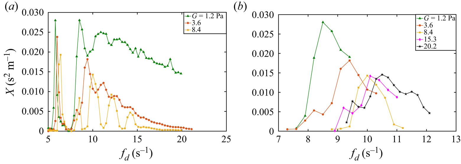
Figure 8. Frequency response, showing amplitude  $X$ against driving frequency
  $f_d$ for (a) the full frequency range and (b) expanded view of the
  $n=2$ mode for agarose gels with shear modulus
  $G$.
$G$.
The resonance frequencies shift to higher values for increasing elasticity  $G$, consistent with our interpretation of elasticity as an additional restorative force in the DDO model. This is illustrated in figure 8(b), which shows the frequency response for the
  $n=2$ mode and shows the resonance peak shifts to higher frequency. The non-monotonic variation in peak
  $X$ with
  $G$ indicates a positive correlation between viscosity and elasticity in agarose gels, whereas a purely elastic response would be monotonic. This correlation between material properties can be proven by rheological measurements on agarose gels which show the magnitude of storage modulus
  $G'$ (elasticity) is always about 10 times larger than that of loss modulus
  $G''$ (viscosity), regardless of the shear modulus.
The frequency response can become complicated for gels with larger elasticity. For example, note the small peak near 8 Hz for the 8.4 Pa gel in figure 8(a), which is actually an additional  $n=2$ resonance peak with smaller peak amplitude than the primary
  $n=2$ peak at approximately 10 Hz. This feature is generally robust for
  $G\geq 3.6$ Pa. Figure 9 shows the frequency response for a
  $G=20.2$ Pa gel showing multiple
  $n=2$ peaks at
  $f_d=8.1$, 10.5 and 13.1 Hz and multiple
  $n=3$ peaks at
  $f_d=9.5$, 11.5, 14.3 and 16.7 Hz. These experimental observations are consistent with nonlinear effects (wave–wave interactions) associated with finite-amplitude gravity-capillary waves known as the Benjamin–Feir instability (BFI) (Benjamin Reference Benjamin1967; Benjamin & Feir Reference Benjamin and Feir1967). This is sometimes referred to as a side-band instability or modulation instability (Zakharov & Ostrovsky Reference Zakharov and Ostrovsky2009) and involves nonlinear dispersion of a moderate amplitude wave packet. Another possible explanation for this observation is the combination resonances discussed by Kidambi (Reference Kidambi2013) for Faraday waves with pinned contact-lines, which is a linear effect from mode coupling. Further studies are needed to investigate this observation on gels and should be pursued.
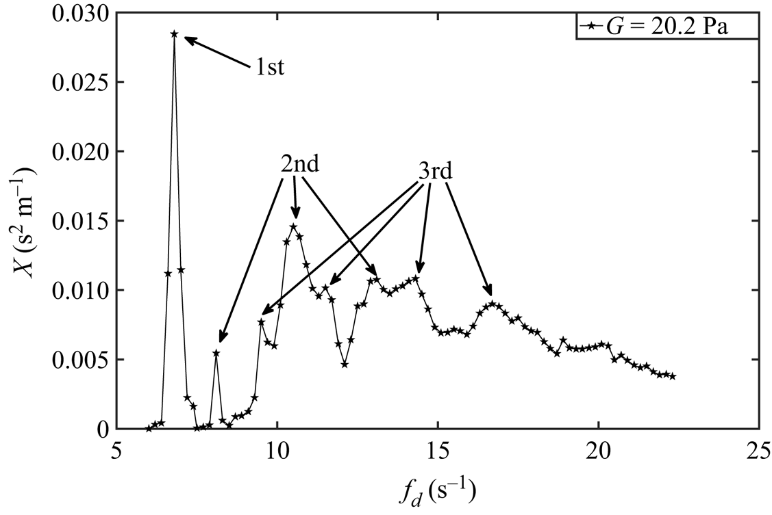
Figure 9. Multiple resonance peaks for a given mode  $n$ are observed in the frequency response showing amplitude
  $X$ against driving frequency
  $f_d$ on an agarose gel with
  $G =20.2$ Pa.
4. Theory of edge waves in a cylindrical container
A viscoelastic fluid fills a cylindrical container of radius  $R$ and height
  $H$ in cylindrical coordinates (
 $r,\theta ,z$), as shown in figure 10. The interface is endowed with surface tension
  $\sigma$ and is given a small axisymmetric disturbance
  $\xi (r,t)$ that is pinned to the lateral sidewall and this generates a flow defined by velocity
  $\boldsymbol {v}$ and pressure
  $p$ fields. Here we apply viscous potential flow theory such that the bulk dissipation from viscosity is approximated by the irrotational flow field (Lamb Reference Lamb1932; Joseph, Funada & Wang Reference Joseph, Funada and Wang2007; Padrino, Funada & Joseph Reference Padrino, Funada and Joseph2007).

Figure 10. Definition sketch.
4.1. Field equations
The fluid is assumed to be incompressible and the flow irrotational, which allows us to define the velocity field  $\boldsymbol {v}=\boldsymbol {\nabla }\varPhi$ through the velocity potential
  $\varPhi$, which satisfies Laplace's equation
 \begin{equation} \nabla^{2} \varPhi = 0,\end{equation}
on the fluid domain, a no-penetration condition
 \begin{equation} \left.\frac{\partial \varPhi}{\partial r}\right|_{r=R}=0,\quad \left.\frac{\partial \varPhi}{\partial z}\right|_{z=0}=0, \end{equation}
at the walls of the cylindrical container and a kinematic condition
 \begin{equation} \frac{\partial \varPhi}{\partial z} = \frac{\partial \xi}{\partial t} \end{equation}
on the free surface  $z=H$, which relates the normal velocity to the perturbation amplitude there. The pressure field is given by the linearised Bernoulli equation
 \begin{equation} p ={-}\rho \frac{\partial \varPhi}{\partial t} - \rho g\xi,\end{equation}
where  $\rho$ is the fluid density and
  $g$ is the gravitational constant. The jump in normal stress at the free surface is governed by the linearised Young–Laplace equation
 \begin{equation} p - 2\mu \frac{\partial^{2} \varPhi}{\partial z^{2}}={-}\frac{\sigma}{R^{2}} \left(\frac{\partial^{2} \xi}{\partial r^{2}}+\frac{1}{r}\frac{\partial \xi }{\partial r}\right), \end{equation}
valid for small disturbances  $|\xi |\ll 1$ with
  $\mu$ the viscosity. The pinned contact-line condition restricts the interface disturbance
  $\xi$ such that
 \begin{equation} \xi|_{r=R}=0. \end{equation}
Lastly, volume conservation is enforced by the integral condition
 \begin{equation} \int_0^{R}{r \xi(r) \,\mathrm{d}r}=0 . \end{equation}
Equations (4.1)–(4.7) define the linearised disturbance equations.
4.2. Reduced equations
The following dimensionless variables are introduced:
 \begin{align} \bar{r}=r/R,\quad \bar{z}=z/R,\quad \bar{\xi}=\xi/R,\quad \bar{t}=t \sqrt{\frac{\sigma}{\varrho r^{3}}},\quad \bar{\varPhi}=\varPhi \sqrt{\frac{\rho}{\sigma R}},\quad \bar{p}=p \left(\frac{R}{\sigma}\right). \end{align}
Here lengths are scaled by the radius of the cylinder  $R$, time with the capillary time scale
  $\sqrt {\rho R^{3}/\sigma }$ and pressure with the capillary pressure
  $\sigma /R$.
Normal modes,
 \begin{equation} \varPhi\left(\boldsymbol{x},t\right)=\phi(r,z)\,\mathrm{e}^{\textrm{i}\omega t},\quad \xi(r,\theta,t)=y(r)\,\mathrm{e}^{\textrm{i}\omega t}, \end{equation}
are assumed with  $\omega$ the oscillation frequency. Viscoelasticity enters the governing equations by introducing the complex viscosity
  $\mu \rightarrow \mu +G/\textrm {i}\omega$, with
  $G$ the shear modulus (Harden, Pleiner & Pincus Reference Harden, Pleiner and Pincus1991). Here we assume that
  $\mu$ and
  $G$ are constants, which is a good approximation for soft polymeric gels (Tokita & Hikichi Reference Tokita and Hikichi1987), but not always the case for materials with a more complex frequency-dependent rheology.
Equations (4.8a–f) and (4.9a,b) are applied to the governing equations (4.1)–(4.6) to yield the domain equations
 $$\begin{gather} \frac{1}{r}\frac{\partial}{\partial r}\left(r \frac{\partial \phi}{\partial r}\right) + \frac{\partial^{2}\phi}{\partial z^{2}} = 0, \end{gather}$$
 $$\begin{gather}p ={-}\textrm{i}\lambda \phi - {Bo}\, y, \end{gather}$$
with boundary conditions on the solid support
 \begin{equation} \left.\frac{\partial \phi}{\partial r}\right|_{r=1}=0,\quad \left.\frac{\partial \phi}{\partial z}\right|_{z=0}=0,\quad y|_{r=1}=0, \end{equation}
and free surface  $z=h$,
 \begin{equation} p-2 \left({Oh}+\frac{{Ec}}{i\lambda}\right) \frac{\partial^{2}\phi}{\partial z^{2}}={-}\left(\frac{\partial^{2} y}{\partial r^{2}}+ \frac{1}{r}\frac{\partial y }{\partial r}\right),\quad \frac{\partial \phi}{\partial z}=i\lambda y. \end{equation}
Here  $\lambda \equiv \omega \sqrt {\rho R^{3}/\sigma }$ is the scaled frequency,
  $h\equiv H/R$ the cylinder aspect ratio,
  ${Bo}\equiv \rho g R^{2}/\sigma$ the Bond number,
  ${Oh}\equiv \mu /\sqrt {\rho R \sigma }$ the Ohnesorge number and
  ${Ec}\equiv GR/\sigma$ the elastocapillary number. The volume-conservation constraint (4.7) requires
 \begin{equation} \int_0^{1}{r y(r)\,\mathrm{d}r}=0. \end{equation}
4.3. Integrodifferential equation
Equations (4.10)–(4.12a,b) can be manipulated into a single integrodifferential equation for the interface disturbance  $y$ by mapping the problem to the interface. Here we write the general solution for
  $\phi$ as
 \begin{equation} \phi (r,z) = \sum_{n = 1}^{\infty} {{A_n}\cosh ({k_{n}}z){J_0}({k_{n}}r)}, \end{equation}
where  $k_{n}$ is the
  $n$th zero of
  ${J'_0}(k)$, as required to satisfy the no-penetration condition at the lateral side wall, with
  $J_0$ the Bessel function. Note that the no-penetration condition at the bottom of the container
  $z=0$ is naturally satisfied by this solution. The interface disturbance
  $y$ can also be expanded in a Bessel function series,
 \begin{equation} y(r) = \sum_{n = 1}^{\infty} {{C_n}{J_0}({k_{n}}r)},\quad {C_n} = \frac{{\left\langle {y,{J_0}({k_{n}}r)} \right\rangle }}{{\left\langle {{J_0}({k_{n}}r),{J_0}({k_{n}}r)} \right\rangle }}, \end{equation}
where the inner product is defined as
 \begin{equation} \left\langle {f(r),g(r)} \right\rangle = \int_0^{1} r f(r)g(r)\,{\textrm{d}}r. \end{equation}
The coefficients  $A_n,C_n$ are related by the kinematic condition,
  $A_n=i\lambda C_n/k_{n} \sinh (k_{n} h)$, and this gives the solution for the velocity potential
 \begin{equation} \phi (r,z) = \textrm{i}\lambda \sum_{n = 1}^{\infty} {\frac{1}{{{k_{n}}}} \frac{{\cosh ({k_{n}}z)}}{{\sinh ({k_{n}}h)}} \frac{{\left\langle {y,{J_0}({k_{n}}r)} \right\rangle }}{{\left\langle {{J_0}({k_{n}}r),{J_0}({k_{n}}r)} \right\rangle }}{J_0}({k_{n}}r)}, \end{equation}
written implicitly through  $y$. This solution is applied to the Young–Laplace equation to give
 \begin{align} & {\lambda ^{2}}\sum_{n = 1}^{\infty} {\frac{\coth ({k_{n}}h)}{{{k_{n}}}} \frac{{\left\langle {y,{J_0}({k_{n}}r)} \right\rangle }}{{\left\langle {{J_0}({k_{n}}r),{J_0}({k_{n}}r)} \right\rangle }}{J_0}({k_{n}}r)} \nonumber\\ &\quad -2\textrm{i}\lambda \,{Oh}\sum_{n = 1}^{\infty} {k_n \coth(k_n h) \frac{{\left\langle {y,{J_0}({k_{n}}r)} \right\rangle }}{{\left\langle {{J_0}({k_{n}}r),{J_0}({k_{n}}r)} \right\rangle }}{J_0}({k_{n}}r)} \nonumber\\ &\quad -2 {Ec}\sum_{n = 1}^{\infty} {k_n \coth(k_n h)\frac{{\left\langle {y,{J_0}({k_{n}}r)} \right\rangle }}{{\left\langle {{J_0}({k_{n}}r),{J_0}({k_{n}}r)} \right\rangle }}{J_0}({k_{n}}r)} - {Bo}\, y + \left[ {\frac{{{d^{2} y}}}{{d{r^{2}}}} + \frac{1}{r}\frac{\textrm{d}y}{{dr}}} \right] = 0, \end{align}
which is an integrodifferential equation for the interface disturbance  $y$.
$y$.
4.4. Operator formalism
To facilitate our solution method for the pinned contact-line condition, we rewrite (4.18) as an operator equation
 \begin{equation} {\lambda ^{2}}M[y] + \lambda D[y;{Oh}]+ K[y;{Bo},{Ec}] = 0, \end{equation}
with
 \begin{equation} M[y] \equiv \sum_{n = 1}^{\infty} {\frac{1}{{{k_{n}}}}\coth ({k_{n}}h) \frac{{\left\langle {y,{J_0}({k_{n}}r)} \right\rangle }}{{\left\langle {{J_0}({k_{n}}r),{J_0}({k_{n}}r)} \right\rangle }}{J_0}({k_{n}}r)}, \end{equation}
an integral operator representative of the fluid inertia,
 \begin{equation} D[y;\textrm{Oh}]\equiv{-}2\textrm{i}\ \textrm{Oh}\sum_{n = 1}^{\infty} {k_n \coth(k_n h) \frac{{\left\langle {y,{J_0}({k_{n}}r)} \right\rangle }}{{\left\langle {{J_0}({k_{n}}r),{J_0}({k_{n}}r)} \right\rangle }}{J_0}({k_{n}}r)}, \end{equation}
the dissipation operator and
 \begin{align} K[y;{Bo},{Ec}] &\equiv{-}2\,{Ec}\sum_{n = 1}^{\infty} {k_n \coth(k_n h) \frac{{\left\langle {y,{J_0}({k_{n}}r)} \right\rangle }}{{\left\langle {{J_0}({k_{n}}r),{J_0}({k_{n}}r)} \right\rangle }}{J_0}({k_{n}}r)} \nonumber\\ &\quad - {Bo}\,y + \left[ {\frac{{{{\textrm{d}}^{2}}}}{{{\textrm{d}}{r^{2}}}} + \frac{1}{r}\frac{{\textrm{d}}}{{{\textrm{d}}r}}} \right]y, \end{align}
a differential operator representative of the restorative forces of surface tension, elasticity, and gravity.
4.5. Rayleigh–Ritz method
A Rayleigh–Ritz method is used to construct an approximate solution to the eigenvalue problem (4.19) by building the pinned contact-line condition and volume-conservation condition (4.13) into the function space over which the minimisation is done. This approach has been applied previously to constrained drops by Bostwick & Steen (Reference Bostwick and Steen2009), Bostwick & Steen (Reference Bostwick and Steen2013a) and Bostwick & Steen (Reference Bostwick and Steen2013b).
To define the constrained function space, we begin with a set of functions that satisfy the pinned-edge condition,
 \begin{equation} {S_n}(r) = {J_0}({k_{n}}r) - \frac{{{J_0}({k_{n}})}}{{{J_0}({k_{1}})}}{J_0}({k_{1}}r)\quad n=2,3,\ldots,N. \end{equation}
Note that the summation starts at  $n=2$. It is straightforward to show that the integral constraint (4.13) is naturally satisfied for this choice of basis functions by using the Bessel function identity
  $\int _0^{1}{r J_0(k r)\,\mathrm {d}r}=-J'_0(k)/k^{2}$. Since
  $k_{n}$ was chosen such that
  $J'_0(k)=0$, it follows that
  $\int _0^{1}{r J_0(k_{n} r)\, \mathrm {d}r}=0$, and using linearity gives
  $\int _0^{1}{r S_n^{0}(r)\,\mathrm {d}r}=0$ for all
  $n$. The Gram–Schmidt procedure can be applied to the functions
  $S_n$ in order to generate a set of orthonormal basis functions
  ${V_i}(r)$, where
  $i=1,2,3,\ldots ,N$, such that
  $\int _0^{1} r V_i(r)V_j(r)\,{\textrm {d}}r = \delta _{ij}$ with
  $\delta _{ij}$ the Kronecker delta function, that span the constrained function space. The surface disturbance
  $y$ can be re-expressed using this orthonormal set as
 \begin{equation} y(r) = \sum_{i = 1}^{\infty} {{c_i}V_i(r)}, \end{equation}
and is applied to the operator equation (4.19) after which inner products are taken to yield the matrix equation
 \begin{equation} ({\lambda ^{2}}{\boldsymbol{M}} + \lambda \boldsymbol{D}+ {\boldsymbol{K}}){\boldsymbol{c}} = 0, \end{equation}
 with matrices  $\boldsymbol {M}$,
  $\boldsymbol {D}$, and
  $\boldsymbol {K}$ defined as
 \begin{equation} {\boldsymbol{M}} = \left\langle {M[{V_i}],{V_j}} \right\rangle,\quad {\boldsymbol{D}} = \left\langle {D[{V_i}],{V_j}} \right\rangle,\quad {\boldsymbol{K}} = \left\langle {K[{V_i}],{V_j}} \right\rangle \end{equation}
and  $\boldsymbol {c}$ the coefficient vector.
4.6. Results
The eigenvalue problem (4.25) is solved numerically in the MATLAB programming environment using the function polyeig which delivers the eigenvalue/vector pairs ( $\lambda$,
 $\boldsymbol {c}$). We use a truncation of
  $N=30$ which produces relative eigenvalue convergence of
  $0.01\,\%$. Typical modes are shown in figure 11 where we present the (i) interface deflection (a–c) and (ii) absolute value of the wave-slope field (d–f). The latter can be directly compared with our experimental imaging technique. The mode number
  $n$ can be associated with the number of nodes of the interface disturbance, which appear as low-intensity circles in the wave-slope field. For example, the
  $n=2$ mode has three nodes including one at the pinned contact-line, which appear as three dark circles in the plot of the wave slope (cf. figure 11). Qualitatively, these results compare very well with the experimental results presented in figure 5. The eigenvalue spectrum can be readily computed for any numerical values of the parameters
  ${Bo},{Oh},{Ec},h$. Damping associated with
  ${Oh}>0$ leads to a complex-valued
  $\lambda$, with the real part
  $\textrm {Re}[\lambda ]$ associated with the oscillation frequency and the imaginary part
  $\textrm {Im}[\lambda ]$, the decay rate. Figure 12 plots the complex frequency against
  ${Oh}$ for the case of a purely viscous liquid showing a bifurcation from underdamped
  $\textrm {Re}[\lambda ]\neq 0$ to overdamped
  $\textrm {Re}[\lambda ]=0$ motions. The critical Ohnesorge number
  ${Oh}$ where this bifurcation occurs decreases with increasing mode number
  $n$ indicating that viscous dissipation increases with the mode number
  $n$. This is also seen in the higher decay rates for higher mode numbers shown in figure 12(
 $b$). With regard to the frequency response, overdamped motions lack an associated resonance peak, as shown in the experimental frequency-response diagram for our most viscous liquids (cf. Figure 7a).
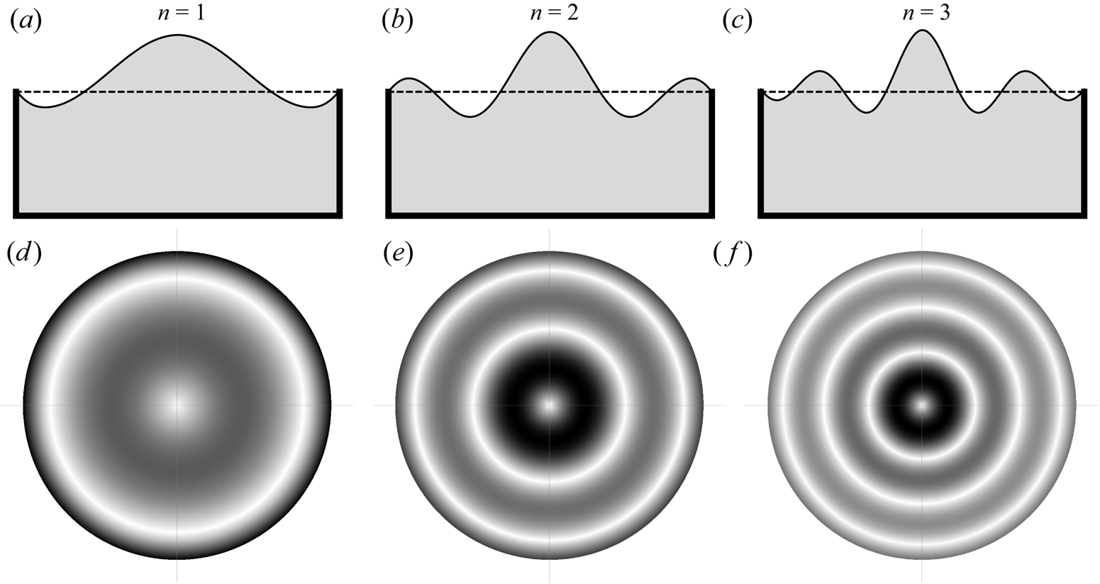
Figure 11. Mode  $n$ shapes (a–c) and associated magnitude of wave slope (d–f).
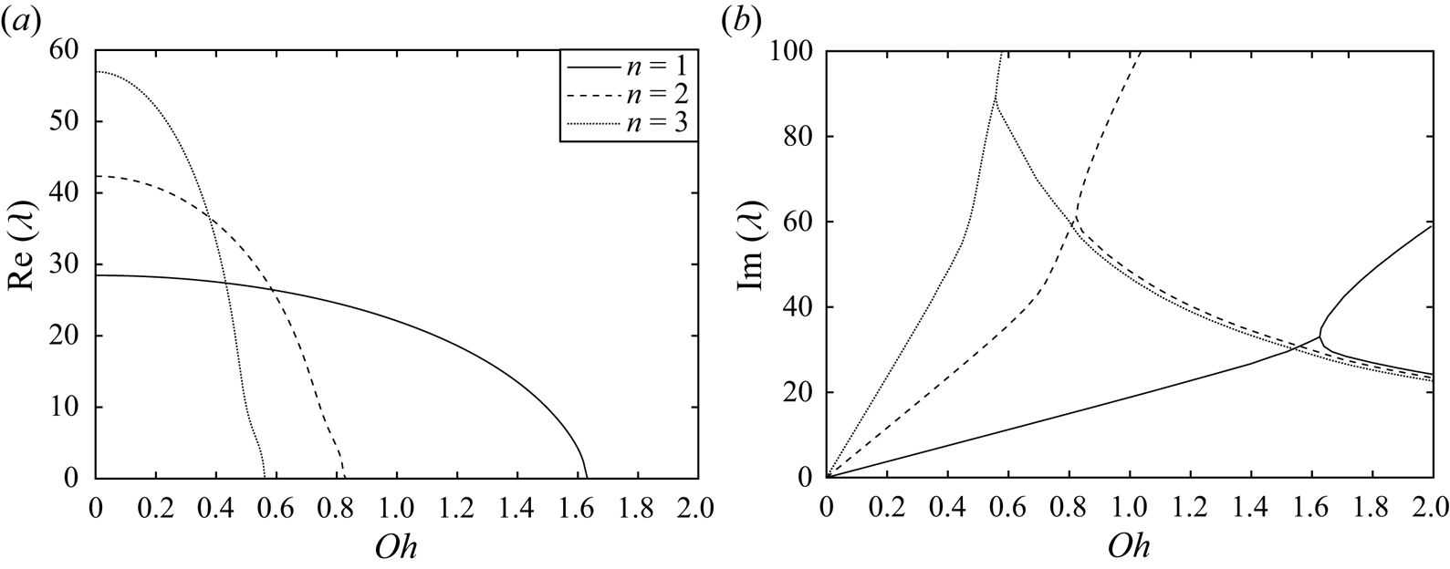
Figure 12. (a) Oscillation frequency  ${Re}[\lambda ]$ and (b) decay rate
  ${Im}[\lambda ]$ against the Ohnesorge number
  ${Oh}$ shows a transition from underdamped to overdamped behaviour for
  ${Bo}=170.8,\ h=0.628,\ {Ec}=0$.
Figure 13 is a plot of the frequency  $\lambda$ against elastocapillary number
  ${Ec}$ for the aspect ratio
  $h=0.628$ and Bond number
  ${Bo}=170.8$ used in our experiments and shows a monotonically increasing trend with
  ${Ec}$ for each mode. Capillary-gravity waves occur in the flat regions and elastocapillary-gravity waves in the regions where the curves are increasing. The transition between these two regions generally occurs near
  ${Ec}\sim 1\text {--}10$, but there is a dependence with mode number
  $n$ that shifts this transition region to higher
  ${Ec}$ with increasing
  $n$. This is because higher mode numbers
  $n$ have smaller wavelengths which are more affected by surface tension with elastic effects less important. Elasticity becomes important when the wavelength
  $\lambda$ is larger than the elastocapillary length
  $\ell _e\equiv \sigma /G$,
  $\lambda > \ell _e$. As
  $\lambda$ decreases with
  $n$, the transition must necessarily occur at larger
  $G$ (i.e. smaller
  $\ell _e$).

Figure 13. Scaled frequency  $\lambda$ against elastocapillary number
  ${Ec}$ for
  ${Oh}=0,h=0.628,{Bo}=170.8$.
4.7. Comparison with experiment
We can compare our theoretical predictions with the experimental resonance peaks shown in figure 7(a) for glycerol/water mixtures and figure 8(a) for agarose gels. Table 2 lists the resonance frequencies for the modes  $n$ observed in the glycerol/water experiments showing good agreement with theory, with all predictions within 10 % of the experimental value. The percent error generally increases with mode number
  $n$ and viscosity
  $\mu$. Table 3 lists the comparison between experiment and theory for the agarose gels. Here we use the largest amplitude resonance peak for each mode number
  $n$, ignoring the nonlinear effects, already discussed, for the stiffest gels. The agreement is good between theory and experiment with most data within 5 % error. Given the large range of viscosity
  ${Oh}$ and elasticity
  ${Ec}$ in our experiments, this level of agreement between theory and experiment suggest that our theoretical development accurately captures the relevant physics present in this viscoelastic system.
Table 2. Experimentally observed resonance frequencies measured in Hertz with deviation from theoretical predictions presented parenthetically for glycerol/water mixtures with material properties listed in table 1.

Table 3. Experimentally observed resonance frequencies measured in Hertz with deviation from theoretical predictions presented parenthetically for agarose gels with  ${Bo}=170.8$.

5. Concluding remarks
We have studied the frequency response of circular edge waves generated in a mechanically vibrated container and focused on viscoelastic effects by using materials that have a tunable (i) viscosity (glycerol/water mixtures) or (ii) elasticity (agarose gels) that remains constant over the range of driving frequencies explored. This is the first experimental observation of edge waves in gels, to our knowledge. Long-exposure time images were used to quantify the magnitude of the wave field through the wave slope and were used to generate frequency-response diagrams from which resonance peaks and associated bandwidths could be readily identified. The spatial structure of the wave is defined by the mode number  $n$ which is readily identified through the wave-slope images. The resonance frequencies for a given mode
  $n$ shift to lower values with increasing viscosity and higher values with increasing elasticity, consistent with our physical interpretation of viscosity as a damping force and elasticity as a restorative force in the classic DDO model. A theoretical model for the natural frequency of a viscoelastic fluid with a flat interface pinned at the edge of a circular container is derived and depends upon the dimensionless Ohnesorge number
  ${Oh}$, Bond number
  ${Bo}$ and elastocapillary number
  ${Ec}$. The model predictions show good agreement with experiment. We note that for the large containers used in our experiments, the meniscus is localised near the container sidewall such that the liquid/gas interface is largely flat across the container diameter. For smaller containers, the meniscus geometry may become more important and affect the natural frequencies. The wave response is more complicated for stiffer gels and the frequency response can exhibit multiple resonance peaks for the same mode number
  $n$ (cf. figure 9). This is consistent with nonlinear wave–wave interactions and the Benjamin–Feir (side-band) instability, but this needs further study.
We note that viscoelastic materials generally exhibit a frequency-dependent rheology, even though the materials we studied were specifically chosen to independently explore viscosity and elasticity. A material with complex rheology will exhibit a crossover frequency, whereby the material response changes from being fluid-like (viscosity) to solid-like (elasticity) and an investigation over a range of driving frequencies that encompass this crossover frequency should be expected to exhibit more complex dynamics. Lastly, we mention that there has been interest in measuring the surface tension of complex materials, particularly those with an elasticity. We note that a method for doing this would be to compare experimental results with theory using surface tension as a free parameter to infer its value.
Funding
J.B.B. acknowledges support from NSF Grants CMMI-1935590, CBET-1750208.
Declaration of interests
The authors report no conflict of interest.


