


1. Introduction
Turbulent and non-turbulent (or weak-turbulent) regions coexist in many flows, such as boundary-layer flow, jet flow and flow past a bluff body. The turbulent/non-turbulent interface is usually unsteady, and the turbulence around the interface is strongly intermittent. Detecting the turbulent/non-turbulent interface is a challenging research topic with a long history of investigations. Various criteria have been proposed to identify such interfaces based on different characteristics of turbulent flows.
The vorticity criterion was proposed to detect the turbulent region based on the fact that turbulence consists of a hierarchy of eddies at various scales (Corrsin & Kistler Reference Corrsin and Kistler1954; Bisset, Hunt & Rogers Reference Bisset, Hunt and Rogers2002; Borrell & Jimémez Reference Borrell and Jimémez2016; Lee & Zaki Reference Lee and Zaki2018). This criterion performs well in the flow region without strong influences of solid walls, such as the far wake region of a boundary-layer flow. However, in the near-wall region, the vorticity associated with the near-wall shear has large magnitude, leading to a misidentification of the non-turbulent region as turbulent. Another important characteristic of turbulent flow is unsteadiness, which motivates the use of velocity fluctuations to detect the turbulent region. In jet flow, the streamwise velocity fluctuation was used as a detector of the turbulent/non-turbulent interface (Anand, Boersma & Agrawal Reference Anand, Boersma and Agrawal2009). The kinetic energy of velocity fluctuations is also an option for detecting the turbulent region in a boundary-layer flow (de Silva et al. Reference de Silva, Philip, Chauhan, Meneveau and Marusic2013; Chauhan et al. Reference Chauhan, Philip, de Silva, Hutchins and Marusic2014). To eliminate the influence of streaky structures diffused from the upstream non-turbulent region in a transitional boundary-layer flow, the magnitude of the wall-normal and spanwise velocity fluctuations was used as a criterion for identifying turbulence (Nolan & Zaki Reference Nolan and Zaki2013). Rehill et al. (Reference Rehill, Walsh, Brandt, Schlatter and Zaki2013) investigated the performances of different criteria in identifying turbulent spots in transitional boundary layers. They examined the criteria based on the instantaneous wall-normal velocity, instantaneous spanwise velocity, value of  $Q$ (Hunt, Wray & Moin Reference Hunt, Wray and Moin1988), value of
  $\lambda _2$ (Jeong & Hussain Reference Jeong and Hussain1995) and gradient of the finite time Lyapunov exponent (Green, Rowley & Haller Reference Green, Rowley and Haller2007). They showed that the turbulent region identified by different criteria are in general consistent, if the threshold values are chosen carefully.
Although the conventional criteria can make a reasonable identification of the turbulent/non-turbulent interface, they have two common limitations. First, as pointed out by Wu et al. (Reference Wu, Lee, Meneveau and Zaki2019b), the choice of threshold value in these criteria is subjective, and, consequently, is highly dependent on the experience of users. Furthermore, most convectional criteria are developed based on one single variable, which usually reflects the turbulent motions at specific characteristic scales. For example, the kinetic energy is mainly contributed by turbulent motions at large scales, while the vorticity is dominated by turbulent motions at smaller scales. However, turbulence is a multiscale physical phenomenon. Therefore, an ideal criterion should contain a combination of multiple flow quantities as the input.
To avoid the above two limitations in the conventional methods, the machine learning method is useful. In recent years, machine learning has been used to study many problems in fluid mechanics, including turbulence modelling (Ling & Templeton Reference Ling and Templeton2015; Ma, Lu & Tryggvason Reference Ma, Lu and Tryggvason2015; Ling, Kurzawski & Templeton Reference Ling, Kurzawski and Templeton2016b; Parish & Duraisamy Reference Parish and Duraisamy2016; Xiao et al. Reference Xiao, Wu, Wang, Sun and Roy2016; Gamahara & Hattori Reference Gamahara and Hattori2017; Vollant, Balarac & Corre Reference Vollant, Balarac and Corre2017; Wang, Wu & Xiao Reference Wang, Wu and Xiao2017; Wang et al. Reference Wang, Luo, Li, Tan and Fan2018; Wu, Xiao & Paterson Reference Wu, Xiao and Paterson2018; Duraisamy, Iaccarino & Xiao Reference Duraisamy, Iaccarino and Xiao2019; Wu et al. Reference Wu, Xiao, Sun and Wang2019a; Zhou et al. Reference Zhou, He, Wang and Jin2019), flow field reconstruction and prediction (Maulik & San Reference Maulik and San2017; Maulik et al. Reference Maulik, San, Rasheed and Vedula2018; Fukami, Fukagata & Taira Reference Fukami, Fukagata and Taira2019; Huang, Liu & Cai Reference Huang, Liu and Cai2019; Lee & You Reference Lee and You2019) and, more relevant to the present study, flow field identification (Colvert, Alsalman & Kanso Reference Colvert, Alsalman and Kanso2018; Alsalman, Colvert & Kanso Reference Alsalman, Colvert and Kanso2019; Wu et al. Reference Wu, Lee, Meneveau and Zaki2019b). To solve the identification problems, there are two main machine learning approaches, namely, classification and clustering. The classification approach is a supervised machine learning method. The training samples are given together with a label to train the classifier. The label provides the classification based on human experiences. Once the training process is finished, the classifier can be used to classify a given sample automatically. An example of the application of the classification method in fluid mechanics is the classifier of wake pattern in the flow past an airfoil by Colvert et al. (Reference Colvert, Alsalman and Kanso2018) and Alsalman et al. (Reference Alsalman, Colvert and Kanso2019). They used a neural network to train the classifier for classifying the wake pattern generated by different motions of the airfoil. The second approach, clustering method, is an unsupervised machine learning method. Unlike the classification method, the clustering method does not need any label as the input information. The clustering algorithm defines the ‘distance’ among input samples in the state space, and clusters them into a specified number of groups. Wu et al. (Reference Wu, Lee, Meneveau and Zaki2019b) used a self-organizing map (SOM) algorithm to cluster the flow field of a transitional boundary layer into turbulent and non-turbulent regions. They showed that these two regions identified by the clustering method are consistent with the visual appearance.
Compared with the conventional methods for turbulence detection, the machine learning method has the advantage of being able to avoid specifying any threshold values explicitly (Wu et al. Reference Wu, Lee, Meneveau and Zaki2019b), which results in a more objective identification. Another advantage of machine learning lies in its capability in processing multiple input variables. As noted by Wu et al. (Reference Wu, Xiao and Paterson2018), most machine learning algorithms are able to handle inputs with more than 1000 features in an efficient manner. In other words, the aforementioned two limitations in the conventional methods for turbulence detection can be well addressed by machine learning.
Inspired by the pioneering work of Wu et al. (Reference Wu, Lee, Meneveau and Zaki2019b), we propose to use machine learning to detect the turbulent region in the wake flow behind a circular cylinder. The present problem is challenging due to the presence of flow separation and unsteady vortex shedding. Because the mean flow direction changes with the location in the flow past a circular cylinder, we propose to use the invariants of the flow as the input of the detector to avoid specifying the reference frame of coordinates. This differs from the choice of the components of velocity and velocity gradients by Wu et al. (Reference Wu, Lee, Meneveau and Zaki2019b) in the boundary-layer flow. The importance of using invariants in machine learning is elucidated in previous studies of turbulence modelling by Ling, Jones & Templeton (Reference Ling, Jones and Templeton2016a) and Wu et al. (Reference Wu, Xiao and Paterson2018). Extreme gradient boosting (XGBoost), a supervised classification method, is used to train the detector, which is applied to identify the turbulent/non-turbulent interface in the wake of a cylinder. The robustness and objectiveness of the trained detector are verified through systematic tests. The XGBoost also shows its novelty in terms of assisting in data analyses. Through the investigation of the feature importance given by XGBoost, the key invariants for quantifying the important transport processes of turbulent flows are further identified.
The remainder of this paper is organized as follows. In § 2, the database used for training and validating the detector is introduced. The training methods are described in § 3. The test results and discussions on the performances of the detectors are presented in § 4. In § 5, physical processes corresponding to the key invariants for turbulence detection are discussed through further analyses of the machine learning results, followed by the conclusions in § 6.
2. Database
2.1. Parameters of numerical simulation
The detector of the turbulent region in the flow past a circular cylinder is trained and validated using the data obtained from direct numerical simulation (DNS) and large-eddy simulation (LES). Figure 1 illustrates the computational domain and coordinates of the simulations. As shown,  $x$,
$x$,  $y$ and
  $z$ denote the streamwise, cross-flow and spanwise directions, respectively. In the
  $x$–
$x$– $y$ plane, the origin of the coordinates is located at the centre of the cylinder. The computational domain size is
  $L_x\times L_y \times L_z = 50D \times 30D \times 3.2 D$, where
  $D$ is the diameter of the cylinder. The inlet of the computational domain is
  $13.5D$ away from the centre of the cylinder. The number of grid points is
  $N_x \times N_y \times N_z = 768 \times 512 \times 256$. Around the cylinder, 80 grid points are used within each diameter of the cylinder in the
  $x$- and
  $y$-directions, giving a resolution of
  $\varDelta _x = \varDelta _y = 1.25\times 10^{-2}D$. The region with the finest grid resolution is shown using the dashed box in figure 1(b). To show the refined region clearly, only part of the computational domain is plotted in figure 1(b). The grid is stretched gradually to the ends of the computational domain in the
  $x$–
$x$– $y$ plane. In the
  $z$-direction, the grid is evenly spaced, and the resolution is
  $\varDelta _z = 1.25\times 10^{-2}D$.
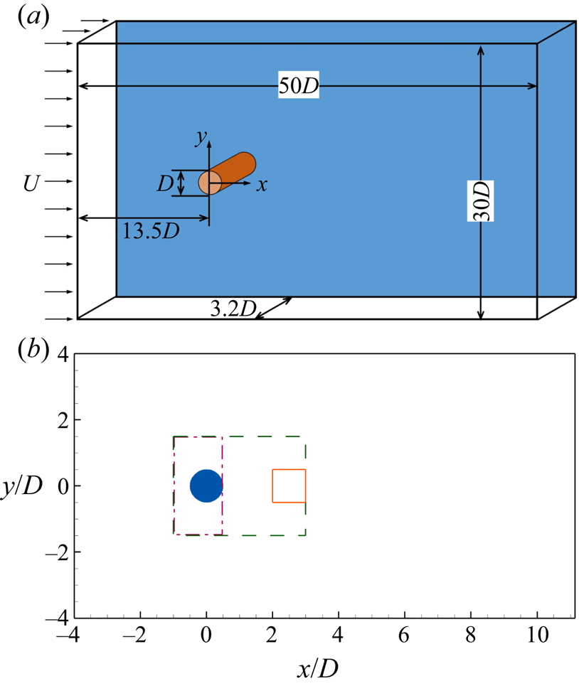
Figure 1. Computational domain and coordinate system of DNS and LES of flow past a circular cylinder. (a) Three-dimensional view and (b) two-dimensional view in an  $x$–
$x$– $y$ plane near the cylinder. The boxes in panel (b) show the regions where training samples are chosen. The samples for the non-turbulent state are chosen from the dashed box for
  $Re=100$ and the dash-dotted box for
  $Re=3900$. The turbulent samples are chosen from the solid box for
  $Re=3900$.
The simulations were conducted by solving the Navier–Stokes equations for incompressible flows using DNS and LES. In the  $x$-direction, the inflow velocity is uniform, and a convective condition is applied at the outlet. The boundary conditions in the
  $y$- and
  $z$-directions are free-slip and periodic, respectively. A second-order central difference scheme is utilized for spatial discretization, and a second-order Runge–Kutta method is employed for time integration. A sharp-interface immersed-boundary method is used to capture the geometry of the cylinder. The details of the numerical methods are given in Cui et al. (Reference Cui, Yang, Jiang, Huang and Shen2018).
We have run simulations of two cases for  $Re = UD/\nu = 100$ and 3900, respectively, where
  $U$ is the inflow velocity and
  $\nu$ is the kinematic viscosity. The flow for
  $Re=100$ is non-turbulent, while the wake region of the flow for
  $Re=3900$ is turbulent. Owing to the coexistence of turbulent and non-turbulent regions at
  $Re=3900$, this case is suitable for examining the proposed method for turbulence detection. The dynamic Smagorinsky model (Germano et al. Reference Germano, Piomelli, Moin and Cabot1991; Lilly Reference Lilly1992) is used to calculate the subgrid-scale stresses in the case for
  $Re = 3900$, while no subgrid-scale model is needed in the case for
  $Re = 100$. We note here that while DNS is ideal for generating the data, it is unfeasible to conduct DNS for the
  $Re=3900$ case due to the limitation in the computational power. However, the data for training the detectors are all chosen inside the dashed box in figure 1(b), where the grid resolution is high. Specifically, the value of
  $\varDelta / \eta$ is smaller than 2.0 inside the dashed box, where
  $\varDelta = (\varDelta _x \varDelta _y \varDelta _z)^{1/3}$ is the grid size and
  $\eta$ is the Kolmogorov length scale. We have also examined the value of the subgrid-scale eddy viscosity inside the box, and found it to be two orders of magnitude smaller than the kinematic viscosity, indicating that the simulation inside the box is essentially DNS. Previous numerical studies of flow past a circular cylinder also indicate that LES can make reliable predictions on the dominant large-scale physical processes, including vortex shedding and transition (Kravchenko & Moin Reference Kravchenko and Moin2000). Therefore, we believe that the data resolution is sufficient to capture the main flow physics in the wake of a circular cylinder. Actually, in many flows in nature, such as oceanic and atmospheric flows, the data obtained from either numerical simulation or field measurement cannot resolve the Kolmogorov length scale. Therefore, detecting turbulence with under-resolved data is an important research topic, which is rather challenging due to the lack of information of small-scale turbulent motions and the uncertainty in the flow data. Haller (Reference Haller2002) proposed methods for detecting Lagrangian structures using the Okubo–Weiss criterion and finite-time Lyapunov exponents, and found that even though a large error may exist in the flow data, the predictions on Lagrangian coherent structures are reliable. In the present study, we focus on turbulent detection with well-resolved data as in most previous studies in the context of Eulerian approaches.
2.2. Validation of LES data
Before proceeding to apply the machine learning method for turbulence detection, it is necessary to examine the quality of the LES data. The turbulent statistics are validated against the experimental results of Lourenco & Shih (see Ma, Karamanos & Karniadakis Reference Ma, Karamanos and Karniadakis2000) and numerical results of Kravchenko & Moin (Reference Kravchenko and Moin2000). Figure 2 shows the profiles of the mean square of streamwise velocity fluctuations  $\overline {u^\prime u^\prime }$ at three locations,
  $x/D=1.06$, 1.54 and 2.02, respectively, in the wake of a circular cylinder at
  $Re=3900$. The prime denotes fluctuations, defined as
  $\phi ^\prime = \phi - \bar {\phi }$, where
  $\phi$ is an arbitrary physical variable, and the overline represents time averaging. It is seen from the figure that the present results are in agreement with previous numerical and experimental results. We have also examined other quantities including the mean streamwise velocity
  $\bar {u}$ and mean cross-flow velocity
  $\bar {v}$. The results are also in good agreement with previous results. We note here that the novelty of the numerical scheme for conducting DNS and LES is not the focus of the present study. We choose the second-order spatial discretization scheme with the incorporation of the immersed-boundary method because of its high computational speed. As we use a fine grid resolution that resolves the Kolmogorov length scale near the cylinder, we generate reliable data of flow field for the present study of turbulence detection.

Figure 2. Transverse profiles of the mean square of streamwise velocity fluctuations  $\overline {u^\prime u^\prime }$ at three downstream locations in the wake of a circular cylinder at
  $Re=3900$.
3. Detector training
3.1. Input features
In the present study, we propose to use flow invariants as the input features for turbulence detection. The input vector  $\boldsymbol {X}$ consists of eight features,
 \begin{align} \boldsymbol{X} & = [X_0,X_1,\ldots\ldots,X_7] \nonumber\\ &=[k,I_2(\boldsymbol{S}^\prime),I_3(\boldsymbol{S}^\prime), I_2(\boldsymbol{\varOmega}^\prime), \nonumber\\ &\qquad\ I_2(\boldsymbol{S}^\prime \boldsymbol{\cdot} \boldsymbol{S}^\prime), I_3(\boldsymbol{S}^\prime \boldsymbol{\cdot} \boldsymbol{S}^\prime), I_2(\boldsymbol{\varOmega}^\prime \boldsymbol{\cdot} \boldsymbol{\varOmega}^\prime), I_2(\boldsymbol{S}^\prime \boldsymbol{\cdot} \boldsymbol{\varOmega}^\prime+ \boldsymbol{\varOmega}^\prime \boldsymbol{\cdot} \boldsymbol{S}^\prime)] , \end{align}
where  $k= u_i^\prime u_i^\prime / 2$ is the kinetic energy of instantaneous velocity fluctuations;
  $I_i(\,)$ denotes the
  $i$-th invariant of a tensor;
  $\boldsymbol {S}^\prime = (\boldsymbol {A}^\prime + \boldsymbol {A}^{\prime \textrm {T}})/2$ and
  $\boldsymbol {\varOmega }^\prime = (\boldsymbol {A}^\prime - \boldsymbol {A}^{\prime \textrm {T}})/2$ are the fluctuations of the strain-rate tensor and rotation-rate tensor, respectively, with
  $\boldsymbol {A}^\prime = \boldsymbol {\nabla } \boldsymbol {u}^\prime$ being the gradient tensor of velocity fluctuations. The superscript ‘T’ represents the transpose of a matrix. Note that we have considered all invariants of the first- and second-order algebraic polynomials of
  $\boldsymbol {S}^\prime$ and
  $\boldsymbol {\varOmega }^\prime$. However, each input sample includes only eight features, because some invariants are trivial. Specifically, the values of some invariants are zero (for example,
  $I_1(\boldsymbol {S}^\prime ) \equiv 0$) and some invariants are not independent (for example,
  $I_1(\boldsymbol {S}^\prime \boldsymbol {\cdot } \boldsymbol {S}^\prime ) \equiv -2I_2(\boldsymbol {S}^\prime )$). Each feature is normalized by its standard deviation over all samples. Besides the eight input features, a supervising label
  $L$ is needed as an input in the supervised classification methods. If the flow state is known as ‘non-turbulent’ or ‘turbulent’, the value of
  $L$ is given as 0 or 1, respectively.
3.2. Mathematical background of the choice of input features
The input features are chosen based on flow physics. In this section, we introduce the physical background of the choice of input features. To capture characteristic physical processes of turbulent flows, we determine the input features according to the following governing equation of the velocity fluctuation:
 \begin{equation} \frac{\partial \boldsymbol{u}^\prime}{\partial t} = - \boldsymbol{u}^\prime \boldsymbol{\cdot} \boldsymbol{\nabla} \bar{\boldsymbol{u}} - \bar{ \boldsymbol{u}} \boldsymbol{\cdot} \boldsymbol{\nabla} \boldsymbol{u}^\prime - \boldsymbol{\nabla} \boldsymbol{\cdot} (\boldsymbol{u}^\prime \boldsymbol{u}^\prime) + \boldsymbol{\nabla} \boldsymbol{\cdot} \overline{\boldsymbol{u}^\prime \boldsymbol{u}^\prime} - \frac{\boldsymbol{\nabla} p}{\rho} + \nu {\rm \Delta} \boldsymbol{u}^\prime , \end{equation}
where  $p$ represents the pressure,
  $\rho$ and
  $\nu$ are the density and kinetic viscosity of the fluid, respectively, and
  $\varDelta = \boldsymbol {\nabla } \boldsymbol {\cdot } \boldsymbol {\nabla }$ is the Laplacian operator. In (3.2), there are two important tensors
  $\boldsymbol {u}^\prime \boldsymbol {u}^\prime$ and
  $\overline {\boldsymbol {u}^\prime \boldsymbol {u}^\prime }$. The former one,
  $\boldsymbol {u}^\prime \boldsymbol {u}^\prime$, has one non-trivial invariant, i.e. the first invariant
  $I_1(\boldsymbol {u}^\prime \boldsymbol {u}^\prime ) = 2k$. As a result, the kinetic energy of the velocity fluctuation
  $k$ is chosen as an input feature. The latter one,
  $\overline {\boldsymbol {u}^\prime \boldsymbol {u}^\prime }$, is not considered for turbulence detection, because it is a time-averaged quantity, but the flow state should be time dependent. For the same reason, the gradient of the mean flow
  $\boldsymbol {\nabla } \bar {\boldsymbol {u}}$ is not considered. Further from (3.2), it is understood that the fluctuation of the velocity gradient tensor
  $\boldsymbol {\nabla } \boldsymbol {u}^\prime$ also participates in the transport of the velocity fluctuation. To choose the invariants corresponding to
  $\boldsymbol {\nabla } \boldsymbol {u}^\prime$, we decomposed it into the symmetric part
  $\boldsymbol {S}^\prime$ and anti-symmetric part
  $\boldsymbol {\varOmega }^\prime$. Therefore, the invariants of
  $\boldsymbol {S}^\prime$ and
  $\boldsymbol {\varOmega }^\prime$ are chosen as the input features. To choose more input features, we consider the transport equations of
  $\boldsymbol {S}^\prime$ and
  $\boldsymbol {\varOmega }^\prime$, which can be written, respectively, as
 \begin{align} \frac{\mathrm{D} \boldsymbol{S}^\prime}{\mathrm{D} t} &= - \boldsymbol{u}^\prime \boldsymbol{\cdot} \boldsymbol{\nabla} \bar{\boldsymbol{S}} - (\bar{\boldsymbol{S}} \boldsymbol{\cdot} \boldsymbol{S}^\prime + \boldsymbol{S}^\prime \boldsymbol{\cdot} \bar{\boldsymbol{S}}) - (\bar{\boldsymbol{\varOmega}} \boldsymbol{\cdot} \boldsymbol{\varOmega}^\prime + \boldsymbol{\varOmega}^\prime \boldsymbol{\cdot} \bar{\boldsymbol{\varOmega}}) - \boldsymbol{S}^\prime \boldsymbol{\cdot} \boldsymbol{S}^\prime - \boldsymbol{\varOmega}^\prime \boldsymbol{\cdot} \boldsymbol{\varOmega}^\prime\nonumber\\ &\quad + \boldsymbol{\nabla}\left(\boldsymbol{\nabla} \boldsymbol{\cdot} \overline{\boldsymbol{u}^\prime \boldsymbol{u}^\prime}\right) - \frac{\boldsymbol{\nabla}(\boldsymbol{\nabla} p)}{\rho} + \nu {\rm \Delta} \boldsymbol{S}^\prime \end{align}
and
 \begin{align} \frac{\mathrm{D} \boldsymbol{\varOmega}^\prime}{\mathrm{D} t} &= - \boldsymbol{u}^\prime \boldsymbol{\cdot} \boldsymbol{\nabla} \bar {\boldsymbol{\varOmega}} - (\bar{ \boldsymbol{S}} \boldsymbol{\cdot} \boldsymbol{\varOmega}^\prime + \boldsymbol{\varOmega}^\prime \boldsymbol{\cdot} \bar{\boldsymbol{S}}) - (\bar{ \boldsymbol{\varOmega}} \boldsymbol{\cdot} \boldsymbol{S}^\prime + \boldsymbol{S}^\prime \boldsymbol{\cdot} \bar{\boldsymbol{\varOmega}}) - (\boldsymbol{S}^\prime \boldsymbol{\cdot} \boldsymbol{\varOmega}^\prime + \boldsymbol{\varOmega}^\prime \boldsymbol{\cdot} \boldsymbol{S}^\prime) \nonumber\\ &\quad + \nu {\rm \Delta} \boldsymbol{\varOmega}^\prime . \end{align}
It is seen that the symmetric tensors  $\boldsymbol {S}^\prime \boldsymbol {\cdot } \boldsymbol {S}^\prime$ and
  $\boldsymbol {\varOmega }^\prime \boldsymbol {\cdot } \boldsymbol {\varOmega }^\prime$ occur in the transport equation of
  $\boldsymbol {S}^\prime$, while the anti-symmetric tensor
  $\boldsymbol {S}^\prime \boldsymbol {\cdot } \boldsymbol {\varOmega }^\prime + \boldsymbol {\varOmega }^\prime \boldsymbol {\cdot } \boldsymbol {S}^\prime$ occurs in the transport equation of
  $\boldsymbol {\varOmega }^\prime$. Therefore, the non-trivial invariants of
  $\boldsymbol {S}^\prime \boldsymbol {\cdot } \boldsymbol {S}^\prime$,
  $\boldsymbol {\varOmega }^\prime \boldsymbol {\cdot } \boldsymbol {\varOmega }^\prime$ and
  $\boldsymbol {S}^\prime \boldsymbol {\cdot } \boldsymbol {\varOmega }^\prime + \boldsymbol {\varOmega }^\prime \boldsymbol {\cdot } \boldsymbol {S}^\prime$ are chosen as the input features. The tensors corresponding to fluid flow are actually unlimited due to the turbulence closure problem. For example, beyond the above second-order algebraic polynomials, the third-order algebraic polynomials
  $\boldsymbol {S}^\prime \boldsymbol {\cdot } \boldsymbol {S}^\prime \boldsymbol {\cdot } \boldsymbol {S}^\prime$,
  $\boldsymbol {S}^\prime \boldsymbol {\cdot } \boldsymbol {\varOmega }^\prime \boldsymbol {\cdot } \boldsymbol {\varOmega }^\prime + \boldsymbol {\varOmega }^\prime \boldsymbol {\cdot } \boldsymbol {\varOmega }^\prime \boldsymbol {\cdot } \boldsymbol {S}^\prime$,
  $\boldsymbol {\varOmega }^\prime \boldsymbol {\cdot } \boldsymbol {S}^\prime \boldsymbol {\cdot } \boldsymbol {\varOmega }^\prime$,
  $\boldsymbol {S}^\prime \boldsymbol {\cdot } \boldsymbol {S}^\prime \boldsymbol {\cdot } \boldsymbol {\varOmega }^\prime + \boldsymbol {\varOmega }^\prime \boldsymbol {\cdot } \boldsymbol {S}^\prime \boldsymbol {\cdot } \boldsymbol {S}^\prime$,
  $\boldsymbol {\varOmega }^\prime \boldsymbol {\cdot } \boldsymbol {\varOmega }^\prime \boldsymbol {\cdot } \boldsymbol {\varOmega }^\prime$ and
  $\boldsymbol {S}^\prime \boldsymbol {\cdot } \boldsymbol {\varOmega }^\prime \boldsymbol {\cdot } \boldsymbol {S}^\prime$ occur on the right-hand side of the transport equations of
  $\boldsymbol {S}^\prime \boldsymbol {\cdot } \boldsymbol {S}^\prime$,
  $\boldsymbol {\varOmega }^\prime \boldsymbol {\cdot } \boldsymbol {\varOmega }^\prime$ and
  $\boldsymbol {S}^\prime \boldsymbol {\cdot } \boldsymbol {\varOmega }^\prime + \boldsymbol {\varOmega }^\prime \boldsymbol {\cdot } \boldsymbol {S}^\prime$. From the test results shown in § 4.5, it is understood that the inclusion of the invariants of the third-order algebraic polynomials of
  $\boldsymbol {S}^\prime$ and
  $\boldsymbol {\varOmega }^\prime$ does not alter the detected turbulent/non-turbulent interface. Therefore, we confine our choice of the tensors up to the second-order algebraic polynomials of
  $\boldsymbol {S}^\prime$ and
  $\boldsymbol {\varOmega }^\prime$.
3.3. Training samples
The turbulence detector is trained using XGBoost, a supervised classification method. The samples used for training and validating the detector must be chosen from the flow region where the flow is known as ‘turbulent’ or ‘non-turbulent’. The samples of non-turbulent flow are chosen from both the  $Re=100$ case and the
  $Re=3900$ case. It is known that at
  $Re=100$, the entire flow field is non-turbulent, while at
  $Re=3900$, the flow field in the upstream of the cylinder is also non-turbulent. Therefore, we choose the flow field in the boxes for
  $(x,y) \in ([-1.0D, 3.0D], [-1.5D, 1.5D])$ (the dashed box in figure 1b) at
  $Re=100$ and
  $(x,y) \in ([-1.0D, 0.5D], [-1.5D, 1.5D])$ (the dash-dotted box in figure 1b) at
  $Re=3900$ as the samples of non-turbulent flow state. The samples of turbulent flow state are all chosen from the case for
  $Re=3900$. According to previous studies of the flow past a circular cylinder at
  $Re = 3900$ (see e.g. Kravchenko & Moin Reference Kravchenko and Moin2000), the transition takes place after flow separation, extending for approximately one cylinder diameter. To choose the samples representing the turbulent flow state, we focus on the wake flow around the centreline of the cylinder for
  $(x,y) \in ([2.0D, 3.0D] , [-0.5D, 0.5D])$ (the solid box in figure 1b), where the flow is known as turbulent. We note here that the turbulent region is actually much larger than the solid box. However, there are two restrictions in the choice of turbulent samples. The first is that the box should be away from the turbulent/non-turbulent interface. If the box is too close to the interface, the non-turbulent samples would be mixed into the turbulent samples due to the wake meandering. The second restriction is the grid resolution. As described in § 2, the grid is refined near the cylinder, and the simulation is essentially DNS in the dashed box in figure 1(b). Therefore, the turbulent samples are confined in the dashed box to minimize the influences of subgrid-scale model. Considering these two restrictions, the solid box is chosen as the representation of the turbulent flow region. We have examined the impact of the choice of turbulent samples on the results of the detected turbulent/non-turbulent interface. It is found that if the flow region for turbulent samples is doubled or halved, the detected turbulent/non-turbulent interface remains almost unchanged. This indicates that the choice of turbulent samples imposes little influence on the detector obtained from the machine learning methods. The details of the test results are shown in § 4.4. We have also tested other machine learning methods, including the full-connected neural network (FCN) and SOM. It is found that XGBoost provides the most reasonable turbulence detection among various machine learning methods. Therefore, in the main content of this paper, we focus on analysing the results of XGBoost, while those of FCN and SOM are given in appendix A.
Once the training process is finished, the detector can be applied at each grid point to identify the flow state at that point. Such a point-by-point method of turbulence detection is similar to Wu et al. (Reference Wu, Lee, Meneveau and Zaki2019b). In some situations, the point-based method may produce small ‘patches’ (unphysical small turbulent regions in non-turbulent flow, see appendix A). Another type of method that is potentially useful for flow identification is a region-based one, which is used by Ströfer et al. (Reference Ströfer, Wu, Xiao and Paterson2019) to identify the vortices in the wake of an airfoil. The region-based method treats flow structures as objects, and as such it does not generate the ‘patches’. However, a region-based method does not provide a sharp edge to the object as the point-based method does; instead, it outputs an approximate region that contains the flow structures of interest.
3.4. Cost function
In the training process, the following cost function is minimized:
 \begin{equation} E = H(L,\hat{L}) + \tfrac{1}{2} ||{\boldsymbol{w}}||^2 , \end{equation}
where  $H(L,\hat {L})$ is the cross-entropy between the values of the supervising label
  $L$ (which is either 0 or 1) and the identification label
  $\hat {L}(s)$ (which is the output of the model, ranging from 0 to 1), defined as
 \begin{equation} H(L,\hat{L}) = - \sum_s \left[ L(s) \log(\hat{L}(s)) + (1- L(s)) \log(1-\hat{L}(s)) \right], \end{equation}
where  $s$ represents the sample index, and the summation is performed over all training samples. Because the value of
  $L$ is either 0 or 1, the cross-entropy can also be expressed as
 \begin{equation} H(L,\hat{L}) = \begin{cases} - \log(1-\hat{L}(s)), & \mathrm{if}\ L=0, \\ - \log(\hat{L}(s)), & \mathrm{if}\ L=1. \end{cases} \end{equation}
From the expression for  $H(L,\hat {L})$, it is known that its value decreases as the value of
  $\hat {L}(s)$ approaches that of
  $L(s)$. The second part of the cost function
  $E$ is used to penalize the complexity of the model. Specifically,
  $\boldsymbol {w} = [w_1, w_2, \ldots ]$ is a vector consisting of trainable variables
  $w_i$ in the model. The value of
  $w_i$ is randomly initialized, and is trained to minimize the cost function
  $E$. The details of the model are described in Chen & Guestrin (Reference Chen and Guestrin2016).
The supervised machine learning method, to some extent, mimics the human learning process. In conventional methods of flow state identification, the flow statistics are first studied. The main differences between the turbulent and non-turbulent regions are then summarized. Based on these investigations, some variables that look the most different between the turbulent and non-turbulent regions, such as kinetic energy or vorticity of velocity fluctuations, together with specified threshold values, are proposed as the criteria for identifying the turbulent/non-turbulent interface. In a supervised machine learning method, the first step is to choose training samples. To minimize the human interference with the machine learning process, the supervising label value of the training samples ( $L=0$ and 1 for non-turbulent and turbulent samples, respectively) should be given without ambiguity. Therefore, as introduced in § 3.3, the training samples in this study are chosen in the flow region away from the turbulent/non-turbulent interface, where the flow state is exactly known according to the knowledge gained from previous studies. After choosing the training samples, the machine learning method is used to train a detector, which outputs an identification label
  $\hat {L}$ ranging from 0 to 1. To apply the detector, the input features at an arbitrary location in the flow field are given to the detector. If the value of the identification label
  $\hat {L}$ is greater than 0.5, it means that the machine learning method ‘thinks’ that the flow at that location is ‘closer’ to the turbulent state; otherwise, the flow state is identified as non-turbulent.
From the above descriptions of the detector, it is understood that the machine learning algorithm essentially identifies the flow state by examining if the testing sample is closer to the turbulent or non-turbulent training samples in the feature space. Although there must exist a threshold between the turbulent and non-turbulent samples, this threshold does not need to be specified explicitly as in the conventional criteria, while instead, it depends implicitly on the samples used for training the detector, of which the flow state is determined according to the knowledge gained from previous studies. Furthermore, the machine learning method can treat multiple input features (eight in the present study) as a combination, while the conventional method is usually proposed based on one or two flow quantities. In these senses, the criteria obtained from machine learning methods are more objective.
3.5. Implementation and hyperparameters of XGBoost
The XGBoost algorithm is compiled into an open source package, of which the Python version is used in the present study. The hyperparameters of XGBoost are summarized in table 1. Note that we only list some of the hyperparameters. If a hyperparameter does not appear in the table, its default value preset in the package is used. The definitions of the hyperparameters of XGBoost are introduced in Chen & Guestrin (Reference Chen and Guestrin2016). In the present study, the hyperparameters are specified to result in the best training accuracy. To be specific, we found that the performance of the detector is mainly influenced by the learning rate, number of trees and the maximum depth of an individual tree. After testing various values of these three hyperparameters, we found an ideal combination of them as listed in table 1, which results in a high training accuracy.
Table 1. Hyperparameters of XGBoost applied in the present study.
The training accuracy can be examined using the confusion matrix as shown in figure 3. The row and column of the matrix represent the labelled and predicted flow states, respectively. The diagonal and off-diagonal entries show the percentages of consistent and inconsistent classifications, respectively. For example, the entry value of the first row and second column gives the percentage of the samples labelled as the non-turbulent state but identified as the turbulent state. It is seen from the figure that the percentage of consistent identifications is greater than  $99\,\%$, indicating a high training accuracy.

Figure 3. Accuracy of the detector trained by XGBoost. Diagonal entries show percentages of consistent classification and off-diagonal entries show percentages of inconsistent classification.
4. Results
4.1. Application to the entire flow field
Using the trained detectors, the instantaneous flow at every grid point can be identified as being in either a turbulent or non-turbulent state. Figure 4 shows the turbulent/non-turbulent interface at  $Re=100$ and
  $Re=3900$ identified by the XGBoost detector. The contours of instantaneous spanwise vorticity
  $\omega _z$ showing the vortex street are superimposed. In figure 4(a), the vortex shedding at
  $Re=100$ is evident from the spanwise vorticity, which, however, should not be identified as turbulent flow. As expected, no turbulent/non-turbulent interface is detected. Figure 4(b) shows that at
  $Re=3900$, the flow on the upstream side of the cylinder is identified as the non-turbulent state. This result is reasonable, as it is known that the transition takes place after the flow separation at this Reynolds number. Downstream, the turbulent region is approximately symmetric about the centreline of the cylinder near the cylinder (
 $x/D<3$), while away from the cylinder (
 $x/D>3$), the turbulent region shows a meandering behaviour.
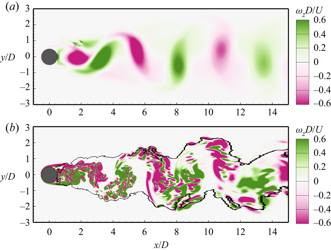
Figure 4. Turbulent/non-turbulent interface (solid line) at (a)  $Re=100$ and (b)
  $Re=3900$ identified by the XGBoost detector. Contours of instantaneous spanwise vorticity
  $\omega _z$ are superimposed for comparison.
Figure 5 further displays successive snapshots of the identified turbulent/non-turbulent interface (solid line) to examine the robustness of detector. The contours of instantaneous spanwise vorticity  $\omega _z$ are also shown. It is seen that in the core region of the wake, the flow is identified as turbulent at every time instant, indicating that the detector is robust in terms of not producing unphysical switching between turbulent and non-turbulent flow states. Near the interface, the flow state alternates between turbulent and non-turbulent due to the wake meandering, a physical process that is evident from the contours of the instantaneous spanwise vorticity.

Figure 5. Successive snapshots of turbulent/non-turbulent interface (solid line) identified by the XGBoost detector and contours of instantaneous spanwise vorticity  $\omega _z$ at
  $Re=3900$. See figure 4 for the legend of contours.
4.2. Application to a higher Reynolds number
The detector is also examined at a higher Reynolds number  $Re=5000$. Although it is desired to examine the performance of the detector in a case at
  $Re>3.5\times 10^6$ with the transition occurring before the flow separation (Williamson Reference Williamson1996), generating high quality data for such a high Reynolds number is unfeasible due to the limitation in the computer power for wall-resolved LES as discussed in § 2. However, because the testing Reynolds number
  $Re=5000$ is higher than the two training Reynolds numbers
  $Re=100$ and 3900, this test to some extent examines the ‘extrapolation robustness’ (with respect to the Reynolds number) of the machine learning method in identifying the turbulent region.
Figure 6 compares the turbulent/non-turbulent interfaces at  $Re=3900$ and 5000. The wake pattern of a circular cylinder varies with the Reynolds number. The two Reynolds numbers under investigation fall into the same subrange (Williamson Reference Williamson1996). Therefore, it is expected to observe similar wake patterns at these two Reynolds numbers. From the figure, it is seen that in the upstream of
  $x/D = 3$, the turbulent region is almost symmetric about the centreline (
 $y/D=0$) of the cylinder, indicating that near the cylinder, the effect of wake meandering on the turbulent/non-turbulent interface is relatively weak. In other words, the turbulent/non-turbulent interface is relatively stable. As a result, the interfaces at the two Reynolds numbers almost collapse. In the downstream of
  $x/D = 3$, the two interfaces start to separate due to the wake meandering. However, the widths of the turbulent region at the two Reynolds numbers are generally consistent. It is noted in previous studies of the jet flow that the growth speed of the turbulent region is independent of the Reynolds number (Bisset et al. Reference Bisset, Hunt and Rogers2002; Westerweel et al. Reference Westerweel, Fukushima, Pedersen and Hunt2009). For the flow past a bluff body, the wake width is found to depend on the local Reynolds number (Johansson & George Reference Johansson and George2003). However, the wake flow is not necessarily turbulent, and further investigations are needed to understand the effect of the Reynolds number on the growth rate of the turbulent/non-turbulent interface, which is not the research topic of the present study. Nevertheless, because the two tested Reynolds numbers are close, it is reasonable to observe that the widths of the turbulent region grow at a similar rate.

Figure 6. Turbulent/non-turbulent interface at  $Re=3900$ (black solid line) and
  $Re=5000$ (red dotted line) identified by the XGBoost detector.
4.3. Comparison with other detection methods
To further demonstrate the novelty of the machine learning method, the XGBoost detector is compared with two detection methods without using the machine learning method, based on the vorticity modulus  $\omega = \sqrt {\omega _i \omega _i}$ (Bisset et al. Reference Bisset, Hunt and Rogers2002) and cross-stream fluctuation intensity
  $|v^\prime |+|w^\prime |$ (Nolan & Zaki Reference Nolan and Zaki2013), respectively, where
  $\omega _i$ is the vorticity in the
  $i$-direction, and
  $|\cdot |$ denotes the absolute value of a real number.
Figure 7 shows the contours of  $\omega$ and
  $|v^\prime |+|w^\prime |$ at
  $Re = 3900$. The turbulent/non-turbulent interface identified by the XGBoost detector is superimposed as the solid line for comparison. The contours for
  $\omega < 0.1U/D$ and
  $|v^\prime |+|w^\prime | < 0.1U$ are clipped. In other words, if
  $\omega = 0.1U/D$ or
  $|v^\prime |+|w^\prime | = 0.1U$ is specified as the threshold value in the conventional criterion, the flow state inside the coloured region in figure 7 is identified as turbulent. It is seen from figure 7 that the edge of the coloured area is in general consistent with the solid line. Inside the solid line, the values of
  $\omega$ and
  $|v^\prime |+|w^\prime |$ are relatively large. However, focusing on the region near the turbulent/non-turbulent interface, it is seen that the spatial variations of both
  $\omega$ and
  $|v^\prime |+|w^\prime |$ are small near the solid line. This indicates that a small change in the threshold values of
  $\omega$ and
  $|v^\prime |+|w^\prime |$ may cause a significant change in the location of the detected turbulent/non-turbulent interface. This issue is well addressed in the machine learning method, in which the threshold value does not need to be specified.

Figure 7. Contours of (a) vorticity modulus  $\omega$ and (b) cross-stream fluctuation intensity
  $|v^\prime |+|w^\prime |$ at
  $Re = 3900$. The solid line shows the turbulent/non-turbulent interface identified by the XGBoost detector. Contours for
  $\omega < 0.1U/D$ and
  $|v^\prime |+|w^\prime | < 0.1U$ are clipped.
To further investigate the behaviour of XGBoost in response to the supervision (or, the label), we have trained another detector, in which the turbulent and non-turbulent samples are no longer chosen from a region with known flow state. Instead, we choose the samples from the dashed box in figure 1(b), where the flow can be either turbulent or non-turbulent. The conventional criterion  $|v^\prime |+|w^\prime |$ is used to label the samples. Specifically, samples with
  $|v^\prime |+|w^\prime | \ge 0.1U$ and
  $|v^\prime |+|w^\prime | < 0.1U$ are labelled as turbulent and non-turbulent states, respectively. For convenience of presentation, we denote this detector as detector
  $B$, while the one described in § 3 is denoted as detector
  $A$.
$A$.
Figure 8(a) shows the confusion matrix of detector  $B$. By contrasting figure 8(a) against figure 3, it is seen that the off-diagonal values of the confusion matrix of detector
  $B$ (
$B$ ( $8.5\,\%$ and
  $2.7\,\%$, respectively) are significantly larger than those of detector
  $A$ (smaller than
  $0.1\,\%$). The difference in the confusion matrix between the two detectors is mainly caused by the choice of the training samples. The training can be regarded as a process for seeking an interface between turbulent and non-turbulent states in the feature space (which has eight dimensions in the present cases). The turbulent and non-turbulent samples for detector
  $A$ are chosen from separate areas in the physical space (figure 1b). Therefore, it can be expected that the interface in the feature space can be relatively ‘sharp’, and as a result the percentages of inconsistent identifications are low. In contrast, the turbulent and non-turbulent samples for detector
  $B$ are connected in the physical space, and as such the interface in the feature space is ‘smeared’, which leads to larger percentages of inconsistent identifications.

Figure 8. Results of detector  $B$. (a) Confusion matrix (see figure 3 for definition); (b) detected turbulent/non-turbulent interface (dashed line). In panel (b), the turbulent/non-turbulent interface identified by detector
  $A$ as described in § 3 (solid line) and the contours of
  $|v^\prime |+|w^\prime |$ at
  $Re=3900$ are superimposed for comparison.
Figure 8(b) compares the turbulent/non-turbulent interface identified by detectors  $A$ and
  $B$. As shown, the two detectors make similar identifications of the turbulent/non-turbulent interface near the cylinder (
 $x/D < 3$). However, in the downstream (
 $x/D>3$), the turbulent region identified by detector
  $B$ is wider than that identified by detector
  $A$. It is also seen from figure 8(b) that inside the dashed line, there are some regions with relatively small values of
  $|v^\prime |+|w^\prime |$ (
 $<0.1U$, where the contours are clipped). The flow states in these regions are identified as turbulent, inconsistent with the label. This is the reason that a relatively large value appears in the off-diagonal entry of the confusion matrix (figure 8a).
It is evident from figure 8 that the turbulent/non-turbulent interface identified by the XGBoost detector is affected by the label of the training samples, indicating that the labels should be given in a rational manner to yield an objective detector. Because an artificial criterion is used to label the samples for training detector  $B$, the results of detector
  $A$ are more objective. Furthermore, to ensure that the influences of the artificial choices for training the detector are minimized, we have examined the effects of the training samples and input features on the predictive result of the turbulent/non-turbulent interface. The results are shown in §§ 4.4 and 4.5, respectively.
4.4. Effect of training samples on the detected turbulent/non-turbulent interface
As noted in § 3.3, the turbulent samples used for detector training are chosen from a box in the core region of the wake (the dashed box in figure 1b). To further investigate the effect of the choice of turbulent samples on the predictive result of the turbulent/non-turbulent interface, we have trained other two detectors, based on smaller and larger boxes, respectively. Figure 9 compares the turbulent regions identified by the XGBoost detector based on different boxes for turbulent samples. The identified turbulent region based on the original box (solid box in the figure) is shown as the coloured area. The turbulent/non-turbulent interface based on a smaller or larger box (dashed boxes in figure 9) is shown as the solid line. It is seen that if the turbulent samples are chosen from a shrunk or expanded region, the detected turbulent region remains almost unchanged. The results shown in figure 9 indicate that the detector is insensitive to the flow region size for choosing the turbulent training samples.

Figure 9. Effect of the training samples on the turbulent region detected by the XGBoost detector. The coloured area shows the detected turbulent region with the turbulent samples chosen from the solid box as described in § 3.3. The solid lines in panels (a) and (b) represent the detected turbulent/non-turbulent interface with the turbulent samples chosen from smaller and larger regions, respectively, as denoted by the dashed boxes in the figure.
4.5. Effect of input features on the detected turbulent/non-turbulent interface
As noted in § 3.2, the numbers of tensors and their invariants are unlimited. Here, we use the advantage of the machine learning method in processing multiple input features to test if the inclusion of more invariants alters the detected turbulent/non-turbulent interface. For this purpose, we define two new input vectors
 \begin{equation} \boldsymbol{X}^* = [\boldsymbol{X} , \boldsymbol{X}^{(a)}] \end{equation}
and
 \begin{equation} \boldsymbol{X}^{**} = [\boldsymbol{X} , \boldsymbol{X}^{(b)}] , \end{equation}
where  $\boldsymbol {X}$ is given by (3.1), while
  $\boldsymbol {X}^{(a)}$ and
  $\boldsymbol {X}^{(b)}$ consist of eight invariants of the second-order algebraic cross-polynomials between the mean strain-rate tensor
  $\bar {\boldsymbol {S}}$ (or mean rotation-rate tensor
  $\bar {\boldsymbol {\varOmega }}$) and fluctuating strain-rate tensor
  $\boldsymbol {S}^\prime$ (or fluctuating rotation-rate tensor
  $\boldsymbol {\varOmega }^\prime$) and 12 invariants of the third-order algebraic polynomials of
  $\boldsymbol {S}^\prime$ and
  $\boldsymbol {\varOmega }^\prime$, respectively. The definitions of
  $\boldsymbol {X}^{(a)}$ and
  $\boldsymbol {X}^{(b)}$ are given, respectively, as
 \begin{align} {}\boldsymbol{X}^{(a)} &= [X_{8},\ldots\ldots,X_{15}] \nonumber\\ & = [I_1(\bar{\boldsymbol{S}} \boldsymbol{\cdot} \boldsymbol{S}^\prime + \boldsymbol{S}^\prime \boldsymbol{\cdot} \bar{\boldsymbol{S}}), I_2(\bar{\boldsymbol{S}} \boldsymbol{\cdot} \boldsymbol{S}^\prime + \boldsymbol{S}^\prime \boldsymbol{\cdot} \bar{\boldsymbol{S}}), I_3(\bar{\boldsymbol{S}} \boldsymbol{\cdot} \boldsymbol{S}^\prime + \boldsymbol{S}^\prime \boldsymbol{\cdot} \bar{\boldsymbol{S}}),\nonumber\\ &\quad\ I_1(\bar {\boldsymbol{\varOmega}} \boldsymbol{\cdot} \boldsymbol{\varOmega}^\prime + \boldsymbol{\varOmega}^\prime \boldsymbol{\cdot} \bar{\boldsymbol{\varOmega}}), I_2(\bar{\boldsymbol{\varOmega}} \boldsymbol{\cdot} \boldsymbol{\varOmega}^\prime + \boldsymbol{\varOmega}^\prime \boldsymbol{\cdot} \bar{\boldsymbol{\varOmega}}), I_3(\bar{\boldsymbol{\varOmega}} \boldsymbol{\cdot} \boldsymbol{\varOmega}^\prime + \boldsymbol{\varOmega}^\prime \boldsymbol{\cdot} \bar{\boldsymbol{\varOmega}}), \nonumber\\ &\quad\ I_2(\bar{\boldsymbol{S}} \boldsymbol{\cdot} \boldsymbol{\varOmega}^\prime + \boldsymbol{\varOmega}^\prime \boldsymbol{\cdot} \bar{\boldsymbol{S}}), I_2(\bar{\boldsymbol{\varOmega}} \boldsymbol{\cdot} \boldsymbol{S}^\prime + \boldsymbol{S}^\prime \boldsymbol{\cdot} \bar{\boldsymbol{\varOmega}})] \end{align}
and
 \begin{align} \boldsymbol{X}^{(b)} & = [X_{16},\ldots\ldots,X_{27}] \nonumber\\ &=[I_1(\boldsymbol{S}^\prime \boldsymbol{\cdot} \boldsymbol{S}^\prime \boldsymbol{\cdot} \boldsymbol{S}^\prime), I_2(\boldsymbol{S}^\prime \boldsymbol{\cdot} \boldsymbol{S}^\prime \boldsymbol{\cdot} \boldsymbol{S}^\prime), I_3(\boldsymbol{S}^\prime \boldsymbol{\cdot} \boldsymbol{S}^\prime \boldsymbol{\cdot} \boldsymbol{S}^\prime), \nonumber\\ &\quad\ I_1(\boldsymbol{\varOmega}^\prime \boldsymbol{\cdot} \boldsymbol{\varOmega}^\prime \boldsymbol{\cdot} \boldsymbol{S}^\prime + \boldsymbol{S}^\prime \boldsymbol{\cdot} \boldsymbol{\varOmega}^\prime \boldsymbol{\cdot} \boldsymbol{\varOmega}^\prime), I_2(\boldsymbol{\varOmega}^\prime \boldsymbol{\cdot} \boldsymbol{\varOmega}^\prime \boldsymbol{\cdot} \boldsymbol{S}^\prime + \boldsymbol{S}^\prime \boldsymbol{\cdot} \boldsymbol{\varOmega}^\prime \boldsymbol{\cdot} \boldsymbol{\varOmega}^\prime),\nonumber\\ &\quad\ I_3(\boldsymbol{\varOmega}^\prime \boldsymbol{\cdot} \boldsymbol{\varOmega}^\prime \boldsymbol{\cdot} \boldsymbol{S}^\prime + \boldsymbol{S}^\prime \boldsymbol{\cdot} \boldsymbol{\varOmega}^\prime \boldsymbol{\cdot} \boldsymbol{\varOmega}^\prime), I_1(\boldsymbol{\varOmega}^\prime \boldsymbol{\cdot} \boldsymbol{S}^\prime \boldsymbol{\cdot} \boldsymbol{\varOmega}^\prime), I_2(\boldsymbol{\varOmega}^\prime \boldsymbol{\cdot} \boldsymbol{S}^\prime \boldsymbol{\cdot} \boldsymbol{\varOmega}^\prime), I_3(\boldsymbol{\varOmega}^\prime \boldsymbol{\cdot} \boldsymbol{S}^\prime \boldsymbol{\cdot} \boldsymbol{\varOmega}^\prime), \nonumber\\ &\quad\ I_2(\boldsymbol{\varOmega}^\prime \boldsymbol{\cdot} \boldsymbol{\varOmega}^\prime \boldsymbol{\cdot} \boldsymbol{\varOmega}^\prime), I_2(\boldsymbol{S}^\prime \boldsymbol{\cdot} \boldsymbol{\varOmega}^\prime \boldsymbol{\cdot} \boldsymbol{S}^\prime), I_2(\boldsymbol{S}^\prime \boldsymbol{\cdot} \boldsymbol{S}^\prime \boldsymbol{\cdot} \boldsymbol{\varOmega}^\prime + \boldsymbol{\varOmega}^\prime \boldsymbol{\cdot} \boldsymbol{S}^\prime \boldsymbol{\cdot} \boldsymbol{S}^\prime)] . \end{align}
 Figure 10 compares the detected turbulent regions using  $\boldsymbol {X}$ (3.1),
  $\boldsymbol {X}^*$ (4.1) and
  $\boldsymbol {X}^{**}$ (4.2) as the input vector. The coloured area represents the turbulent region detected using
  $\boldsymbol {X}$ with eight input features. The solid lines in figures 10(a) and 10(b) show the turbulent/non-turbulent interfaces detected using
  $\boldsymbol {X}^*$ with 16 input features and
  $\boldsymbol {X}^{**}$ with 20 input features, respectively. From both figures 10(a) and 10(b), it is seen that the solid lines are almost coincident with the edges of the coloured areas, indicating that including the invariants of either the second-order algebraic cross-polynomials between
  $\bar {\boldsymbol {S}}$ (or
  $\bar {\boldsymbol {\varOmega }}$) and
  $\boldsymbol {S}^\prime$ (or
  $\boldsymbol {\varOmega }^\prime$) or the third-order algebraic polynomials of
  $\boldsymbol {S}^\prime$ and
  $\boldsymbol {\varOmega }^\prime$ imposes little influence on the predictive results of the turbulent/non-turbulent interface. Therefore, it is sufficient to consider the first- and second-order polynomials of
  $\boldsymbol {S}^\prime$ and
  $\boldsymbol {\varOmega }^\prime$ for turbulence detection in the present study.

Figure 10. Effect of input features on the turbulent region detected by the XGBoost detector. The coloured area shows the detected turbulent region using  $\boldsymbol {X}$ (3.1) as the input vector, which consists of eight features, without including the invariants of third-order algebraic polynomials of
  $\boldsymbol {S}^\prime$ and
  $\boldsymbol {\varOmega }^\prime$. The solid line in panels (a) and (b) represents the detected turbulent/non-turbulent interface using
  $\boldsymbol {X}^*$ (4.1) and
  $\boldsymbol {X}^{**}$ (4.2), respectively, as the input vector.
Note that XGBoost can further output the importance of each feature in the identification of the flow state. Table 2 lists the value of each feature importance in vectors  $\boldsymbol {X}$,
  $\boldsymbol {X}^*$ and
  $\boldsymbol {X}^{**}$. The feature importance can be deemed as an indicator showing how different this feature is between the turbulent and non-turbulent flow states. If the feature importance is large, such as
  $k$,
$k$,  $I_2(\boldsymbol {S}^\prime \boldsymbol {\cdot } \boldsymbol {\varOmega }^\prime )$ and
  $I_3(\boldsymbol {S}^\prime \boldsymbol {\cdot } \boldsymbol {S}^\prime )$, this feature is found to be significantly different between the turbulent and non-turbulent flow states. It is seen from table 2 that the feature importance values of
  $k$,
$k$,  $I_2(\boldsymbol {S}^\prime \boldsymbol {\cdot } \boldsymbol {\varOmega }^\prime + \boldsymbol {\varOmega }^\prime \boldsymbol {\cdot } \boldsymbol {S}^\prime )$ and
  $I_3(\boldsymbol {S}^\prime \boldsymbol {\cdot } \boldsymbol {S}^\prime )$ rank top three in either
  $\boldsymbol {X}$,
  $\boldsymbol {X}^*$ or
  $\boldsymbol {X}^{**}$. This means that
  $k$,
$k$,  $I_2(\boldsymbol {S}^\prime \boldsymbol {\cdot } \boldsymbol {\varOmega }^\prime )$ and
  $I_3(\boldsymbol {S}^\prime \boldsymbol {\cdot } \boldsymbol {S}^\prime )$ are the three key invariants for the robustness of the detector, and as a result, it is necessary to include second-order algebraic polynomials of
  $\boldsymbol {S}^\prime$ and
  $\boldsymbol {\varOmega }^\prime$ for turbulent detection. It is noted that although the inclusion of the second-order algebraic cross-polynomials between
  $\bar {\boldsymbol {S}}$ (or
  $\bar { \boldsymbol {\varOmega }}$) and
  $\boldsymbol {S}^\prime$ (or
  $\boldsymbol {\varOmega }^\prime$) imposes little influence on the identification of the turbulence/non-turbulence interface, the feature importance value of
  $I_2(\boldsymbol {S}^\prime \boldsymbol {\cdot } \bar {\boldsymbol {\varOmega }} + \bar {\boldsymbol {\varOmega }} \boldsymbol {\cdot } \boldsymbol {S}^\prime )$ is comparable to those of
  $k$,
$k$,  $I_2(\boldsymbol {S}^\prime \boldsymbol {\cdot } \boldsymbol {\varOmega }^\prime )$ and
  $I_3(\boldsymbol {S}^\prime \boldsymbol {\cdot } \boldsymbol {S}^\prime )$, indicating that
  $I_2(\boldsymbol {S}^\prime \boldsymbol {\cdot } \bar {\boldsymbol {\varOmega }} + \bar {\boldsymbol {\varOmega }} \boldsymbol {\cdot } \boldsymbol {S}^\prime )$ also shows a significant difference between turbulent and non-turbulent flows. The physical processes corresponding to these four invariants are further discussed in § 5. Furthermore, all invariants of third-order algebraic polynomials have smaller order of magnitude in feature importance than
  $k$,
$k$,  $I_2(\boldsymbol {S}^\prime \boldsymbol {\cdot } \boldsymbol {\varOmega }^\prime )$ and
  $I_3(\boldsymbol {S}^\prime \boldsymbol {\cdot } \boldsymbol {S}^\prime )$, indicating that it is sufficient to use the first- and second-order algebraic polynomials of
  $\boldsymbol {S}^\prime$ and
  $\boldsymbol {\varOmega }^\prime$ to train an objective detector of the turbulent/non-turbulent interface.


5. Physical processes corresponding to the key input features
So far this paper has focused on the performance of the trained detector on the identification of the turbulent/non-turbulent interface in the flow past a circular cylinder at low Reynolds numbers. It is understood that XGBoost suggests  $k$,
$k$,  $I_2(\boldsymbol {S}^\prime \boldsymbol {\cdot } \boldsymbol {\varOmega }^\prime +\boldsymbol {\varOmega }^\prime \boldsymbol {\cdot } \boldsymbol {S}^\prime )$,
  $I_3(\boldsymbol {S}^\prime \boldsymbol {\cdot } \boldsymbol {S}^\prime )$ and
  $I_2( \bar {\boldsymbol {\varOmega }} \boldsymbol {\cdot } \boldsymbol {S}^\prime +\boldsymbol {S}^\prime \boldsymbol {\cdot } \bar {\boldsymbol {\varOmega }})$ as the dominant invariants that are significantly different between turbulent and non-turbulent flow states. In this section, we further investigate the physical processes corresponding to these invariants. For this purpose, their contours are displayed in figure 11. The detected turbulent/non-turbulent interface is superimposed as the solid line.
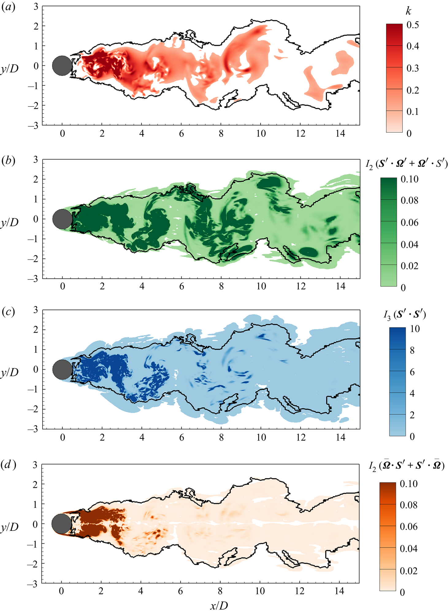
Figure 11. Contours of invariants: (a)  $k$, (b)
  $I_2(\boldsymbol {S}^\prime \boldsymbol {\cdot } \boldsymbol {\varOmega }^\prime +\boldsymbol {\varOmega }^\prime \boldsymbol {\cdot } \boldsymbol {S}^\prime )$, (c)
  $I_3(\boldsymbol {S}^\prime \boldsymbol {\cdot } \boldsymbol {S}^\prime )$ and (d)
  $I_2( \bar {\boldsymbol {\varOmega }} \boldsymbol {\cdot } \boldsymbol {S}^\prime +\boldsymbol {S}^\prime \boldsymbol {\cdot } \bar {\boldsymbol {\varOmega }})$. Contours corresponding to
  $k<10^{-3}U^2$,
  $I_2(\boldsymbol {S}^\prime \boldsymbol {\cdot } \boldsymbol {\varOmega }^\prime +\boldsymbol {\varOmega }^\prime \boldsymbol {\cdot } \boldsymbol {S}^\prime ) <10^{-5}U^4/D^4$,
  $I_3(\boldsymbol {S}^\prime \boldsymbol {\cdot } \boldsymbol {S}^\prime )<10^{-7}U^6/D^6$ and
  $I_2( \bar {\boldsymbol {\varOmega }} \boldsymbol {\cdot } \boldsymbol {S}^\prime +\boldsymbol {S}^\prime \boldsymbol {\cdot } \bar {\boldsymbol {\varOmega }})<10^{-5}U^4/D^4$ are clipped. The solid line represents the detected turbulent/non-turbulent interface.
It is well understood that unsteadiness is a characteristic feature of turbulent flows. Therefore, it is reasonable that the kinetic energy of the velocity fluctuations  $k$ is identified as the most important feature for turbulence detection. As shown in figure 11(a), the magnitude of
  $k$ is relatively large inside the solid line. On the other hand, if the fluctuation is weak, the flow state is identified as non-turbulent.
The second most important feature is  $I_2(\boldsymbol {S}^\prime \boldsymbol {\cdot } \boldsymbol {\varOmega }^\prime +\boldsymbol {\varOmega }^\prime \boldsymbol {\cdot } \boldsymbol {S}^\prime )$. This invariant is equivalent to the norm of the vortex stretching
  $\boldsymbol {\omega }^\prime \boldsymbol {\cdot } \boldsymbol {S}^\prime$, which is known as an important process in turbulent flows. It can be shown that
  $I_2(\boldsymbol {S}^\prime \boldsymbol {\cdot } \boldsymbol {\varOmega }^\prime +\boldsymbol {\varOmega }^\prime \boldsymbol {\cdot } \boldsymbol {S}^\prime ) = ||\boldsymbol {\omega }^\prime \boldsymbol {\cdot } \boldsymbol {S}^\prime ||^2/4$ holds strictly, where
  $\boldsymbol {\omega } = \boldsymbol {\nabla } \times \boldsymbol {u}$ is the vorticity vector and
  $||\boldsymbol {\cdot }||$ denotes the norm of a vector. Figure 11(b) shows that in the turbulent flow region, the value of
  $I_2(\boldsymbol {S}^\prime \boldsymbol {\cdot } \boldsymbol {\varOmega }^\prime +\boldsymbol {\varOmega }^\prime \boldsymbol {\cdot } \boldsymbol {S}^\prime )$ is in general larger than that in the non-turbulent flow region. In the conventional methods of turbulence identification, the norm of vorticity is considered as one of the criteria (Bisset et al. Reference Bisset, Hunt and Rogers2002), but the vortex stretching is overlooked. However, as shown in table 2, the feature importance of
  $I_2(\boldsymbol {S}^\prime \boldsymbol {\cdot } \boldsymbol {\varOmega }^\prime +\boldsymbol {\varOmega }^\prime \boldsymbol {\cdot } \boldsymbol {S}^\prime )$ is larger than that of
  $I_2(\boldsymbol {\varOmega }^\prime ) = ||\omega ^\prime ||^2/4$. This indicates that between turbulent and non-turbulent flow states, the difference in the vortex stretching is more significant than that in the vorticity, and as a result, the vortex stretching is a more effective criterion than the vorticity modulus for turbulence detection.
Although the third most important feature  $I_3(\boldsymbol {S}^\prime \boldsymbol {\cdot } \boldsymbol {S}^\prime )$ is not directly connected with a physical quantity that is broadly investigated in the literature, it can be shown that if the straining is confined in a two-dimensional plane (for example,
  $S_{i3}^\prime =S_{3i}^\prime =0$ in the case of
  $Re=100$), the value of
  $I_3(\boldsymbol {S}^\prime \boldsymbol {\cdot } \boldsymbol {S}^\prime )$ is zero. In contrast, if the straining takes place in three dimensions, the value of
  $I_3(\boldsymbol {S}^\prime \boldsymbol {\cdot } \boldsymbol {S}^\prime )$ is non-zero. Therefore, the value of
  $I_3(\boldsymbol {S}^\prime \boldsymbol {\cdot } \boldsymbol {S}^\prime )$ can be regarded as an indicator of the three-dimensionality of the flow. It is seen from figure 11(c) that the value of
  $I_3(\boldsymbol {S}^\prime \boldsymbol {\cdot } \boldsymbol {S}^\prime )$ is relatively large in the turbulent region. Similar to
  $I_2(\boldsymbol {S}^\prime \boldsymbol {\cdot } \boldsymbol {\varOmega }^\prime +\boldsymbol {\varOmega }^\prime \boldsymbol {\cdot } \boldsymbol {S}^\prime )$,
  $I_3(\boldsymbol {S}^\prime \boldsymbol {\cdot } \boldsymbol {S}^\prime )$ has not been used in conventional criteria for identifying turbulence. This evidently shows the strong capability of the machine learning method in seeking important invariants that have been overlooked in previous studies.
The fourth invariant  $I_2( \bar {\boldsymbol {\varOmega }} \boldsymbol {\cdot } \boldsymbol {S}^\prime +\boldsymbol {S}^\prime \boldsymbol {\cdot } \bar {\boldsymbol {\varOmega }})$ is equivalent to the norm of
  ${\bar {\boldsymbol {\omega }}} \boldsymbol {\cdot } \boldsymbol {S}^\prime$, the vortex stretching induced by the interaction between the mean vorticity
  $\bar {\omega }$ and the fluctuating strain-rate tensor
  $\boldsymbol {S}^\prime$. From the comparison between figures 11(b) and 11(d), it is seen that near the cylinder, the magnitude of
  $I_2( \bar {\boldsymbol {\varOmega }} \boldsymbol {\cdot } \boldsymbol {S}^\prime +\boldsymbol {S}^\prime \boldsymbol {\cdot } \bar {\boldsymbol {\varOmega }})$ is comparable to that of
  $I_2(\boldsymbol {S}^\prime \boldsymbol {\cdot } \boldsymbol {\varOmega }^\prime +\boldsymbol {\varOmega }^\prime \boldsymbol {\cdot } \boldsymbol {S}^\prime )$, indicating the coexistence of two vortex stretching processes associated with mean vorticity and vorticity fluctuations, respectively. However, away from the cylinder, where the magnitude of the mean vorticity is small, the value of
  $I_2( \bar {\boldsymbol {\varOmega }} \boldsymbol {\cdot } \boldsymbol {S}^\prime +\boldsymbol {S}^\prime \boldsymbol {\cdot } \bar {\boldsymbol {\varOmega }})$ is smaller than that of
  $I_2(\boldsymbol {S}^\prime \boldsymbol {\cdot } \boldsymbol {\varOmega }^\prime +\boldsymbol {\varOmega }^\prime \boldsymbol {\cdot } \boldsymbol {S}^\prime )$. This indicates that if
  $I_2( \bar {\boldsymbol {\varOmega }} \boldsymbol {\cdot } \boldsymbol {S}^\prime +\boldsymbol {S}^\prime \boldsymbol {\cdot } \bar {\boldsymbol {\varOmega }})$ is used solely as the criterion, the turbulent region is underestimated. From the above comparison between the contours of
  $I_2( \bar {\boldsymbol {\varOmega }} \boldsymbol {\cdot } \boldsymbol {S}^\prime +\boldsymbol {S}^\prime \boldsymbol {\cdot } \bar {\boldsymbol {\varOmega }})$ and
  $I_2(\boldsymbol {S}^\prime \boldsymbol {\cdot } \boldsymbol {\varOmega }^\prime +\boldsymbol {\varOmega }^\prime \boldsymbol {\cdot } \boldsymbol {S}^\prime )$, it is understood that
  $I_2( \bar {\boldsymbol {\varOmega }} \boldsymbol {\cdot } \boldsymbol {S}^\prime +\boldsymbol {S}^\prime \boldsymbol {\cdot } \bar {\boldsymbol {\varOmega }})$, to some extent, characterizes the difference between turbulent and non-turbulent states in the flow region with strong mean vorticity, while if the mean vorticity is weak,
  $I_2( \bar {\boldsymbol {\varOmega }} \boldsymbol {\cdot } \boldsymbol {S}^\prime +\boldsymbol {S}^\prime \boldsymbol {\cdot } \bar {\boldsymbol {\varOmega }})$ is unimportant for turbulence detection. This point is evident from the feature importance value of
  $I_2( \bar {\boldsymbol {\varOmega }} \boldsymbol {\cdot } \boldsymbol {S}^\prime +\boldsymbol {S}^\prime \boldsymbol {\cdot } \bar {\boldsymbol {\varOmega }})$, which is relatively large among all invariants, but is smaller than that of
  $I_2(\boldsymbol {S}^\prime \boldsymbol {\cdot } \boldsymbol {\varOmega }^\prime +\boldsymbol {\varOmega }^\prime \boldsymbol {\cdot } \boldsymbol {S}^\prime )$ (table 2). Furthermore, the feature importance values of
  $I_2( \bar {\boldsymbol {\varOmega }} \boldsymbol {\cdot } \boldsymbol {S}^\prime +\boldsymbol {S}^\prime \boldsymbol {\cdot } \bar {\boldsymbol {\varOmega }})$ and
  $I_3(\boldsymbol {S}^\prime \boldsymbol {\cdot } \boldsymbol {S}^\prime )$ are close. This is because
  $I_2( \bar {\boldsymbol {\varOmega }} \boldsymbol {\cdot } \boldsymbol {S}^\prime +\boldsymbol {S}^\prime \boldsymbol {\cdot } \bar {\boldsymbol {\varOmega }})$ also diminishes in a two-dimensional flow as
  $I_3(\boldsymbol {S}^\prime \boldsymbol {\cdot } \boldsymbol {S}^\prime )$ does. From the above analyses, it is understood that the role of
  $I_2( \bar {\boldsymbol {\varOmega }} \boldsymbol {\cdot } \boldsymbol {S}^\prime +\boldsymbol {S}^\prime \boldsymbol {\cdot } \bar {\boldsymbol {\varOmega }})$ in the turbulence detection can be well covered by the combination of
  $I_2(\boldsymbol {S}^\prime \boldsymbol {\cdot } \boldsymbol {\varOmega }^\prime +\boldsymbol {\varOmega }^\prime \boldsymbol {\cdot } \boldsymbol {S}^\prime )$ and
  $I_3(\boldsymbol {S}^\prime \boldsymbol {\cdot } \boldsymbol {S}^\prime )$, and as such the turbulent/non-turbulent interfaces identified using
  $\boldsymbol {X}$ and
  $\boldsymbol {X^*}$ as input features almost collapse.
From the above analyses of the key invariants, it is understood that XGBoost suggests turbulent flows be characterized by unsteadiness, vortex stretching and three-dimensionality. Although these characteristics of turbulence are broadly accepted, no criterion has been developed based on the combination of these properties for turbulence detection, because of the following two challenges. First, to develop a criterion, these characteristics need quantitative representations, but the ideal choice based on previous studies is inconclusive. For example, the vortex structures can be estimated by either vorticity or vortex stretching. Owing to its capability in processing multiple input features, XGBoost well solves this problem. There is no need to specify a quantity to represent a characteristic of turbulence. Instead, as is done in the present study, all possible choices can be used together to train the detector, and the XGBoost algorithm is able to identify their importance automatically. The second challenge lies in the threshold value. Taking the kinetic energy of velocity fluctuation  $k$ as an example, as shown in figure 11(a), if
  $k=0.1U^2$ is specified as the threshold value, the area of the turbulent region is underestimated. If this value is decreased, the identified turbulent region tends to expand, but this causes the misidentification of the flow state of non-turbulent samples as turbulent at the lower Reynolds number
  $Re=100$ (not shown in the figure). In other words, the threshold value needs to be adjusted with the Reynolds number to obtain reasonable results, and as such the identification process is highly subjective. The solution to this problem is to include other features in the training process to improve the robustness of the detector, which yields objective and reasonable identifications of the flow states at both
  $Re=100$ and
  $Re=3900$ (figure 4).
6. Conclusions
In the present study, XGBoost is used to train a detector to identify the turbulent/non-turbulent interface in the wake of a circular cylinder at low Reynolds numbers. To obtain a detector that is independent of the reference frame of coordinates, we propose to use invariants of the flow field as the input features to train the detector. The invariants include the instantaneous kinetic energy of velocity fluctuations, and the non-trivial invariants of the first- and second-order polynomials of the fluctuating strain-rate and rotation-rate tensors.
To train the detector, we conduct DNS and LES of the flow past a circular cylinder at  $Re=100$ and 3900, respectively. The non-turbulent samples are chosen from the wake region of the cylinder at
  $Re=100$ and in the upstream of the cylinder at
  $Re=3900$. The turbulent samples are chosen in the core region of the wake, where the flow is known as a turbulent state. After training, the detector is used to identify the flow state point by point. The entire flow field for
  $Re=100$ is identified as a non-turbulent region. This is a desired outcome of a detector for not misidentifying the non-turbulent flow state as the turbulent flow state. The turbulent region for
  $Re=3900$ identified by the XGBoost detector is also reasonable, which shows the wake flow meandering. The detector is found robust in the applications to successive snapshots of the flow field and to a higher Reynolds number
  $Re=5000$. The objectiveness of the method is verified through the examination of the effect of training samples and input features on the predictive results of the turbulent/non-turbulent interface.
Compared with conventional turbulence detection methods, machine learning shows its advantage in two aspects. First, no explicitly specified threshold value is needed in the machine learning method. This reduces the influence of any subjective choice on the results. Second, machine learning is able to handle multiple input variables as a combination, which is particularly important for turbulence detection, because turbulence transport is a multiscale physical process. Owing to these two advantages, machine learning makes more objective and robust identifications of the turbulent/non-turbulent interface.
The XGBoost also shows its capability in identifying important physical processes in turbulent transport. The feature importance given by XGBoost indicates that the three most important invariants that vary distinctively between turbulent and non-turbulent flows are  $k=I_1(\boldsymbol {u}^\prime \boldsymbol {u}^\prime )/2$,
  $I_2(\boldsymbol {S}^\prime \boldsymbol {\cdot } \boldsymbol {\varOmega }^\prime +\boldsymbol {\varOmega }^\prime \boldsymbol {\cdot } \boldsymbol {S}^\prime )$ and
  $I_3(\boldsymbol {S}^\prime \boldsymbol {\cdot } \boldsymbol {S}^\prime )$, which characterize unsteadiness, vortex stretching and three-dimensionality of turbulent flows, respectively. Furthermore, the feature importance of
  $I_2(\boldsymbol {S}^\prime \boldsymbol {\cdot } \boldsymbol {\varOmega }^\prime +\boldsymbol {\varOmega }^\prime \boldsymbol {\cdot } \boldsymbol {S}^\prime ) = ||\boldsymbol {\omega }^\prime \boldsymbol {\cdot }\boldsymbol {S}^\prime ||^2/4$ is larger than that of
  $I_2(\boldsymbol {\varOmega }^\prime ) = ||\boldsymbol {\omega }||^2/4$, indicating that the vortex stretching is a more objective criterion for turbulence detection than the vorticity modulus as used in the conventional methods.
As a final remark of this paper, it should not be expected that the detector trained using data at low Reynolds numbers can be used to identify the turbulent/non-turbulent interface in the cylinder wake at a much higher Reynolds number. The present study focuses on how to obtain a detector that is more objective than conventional criteria, while machine learning is found to be an effective tool for achieving this goal. In this regard, the present work provides an executable method to generate a detector for identifying the turbulent/non-turbulent interface. If reliable data for much higher Reynolds numbers are available (which is unfeasible at the current stage due to the limitation in the computer power), one can first choose new training samples with known flow states from the new data. A new detector can be then trained and applied to the entire flow field to find the turbulent/non-turbulent interface. The same approach can be also extended to turbulence detection of other flows, such as the transitional boundary layer and jet flows.
Acknowledgements
B.L., Z.Y., X.Z. and G.H. would like to thank the supported by the NSFC Basic Science Center Program for ‘Multiscale Problems in Nonlinear Mechanics’ (no. 11988102) and the Strategic Priority Research Program (Grant no. XDB22040104). Z.Y. also acknowledges the ‘Lixing’ Plan of the Institute of Mechanics, Chinese Academy of Sciences.
Declaration of interests
The authors report no conflict of interest.
Appendix A. Detection using other machine learning methods
In the main content of this paper, we present the results of XGBoost. We have also tested other machine learning methods, including FCN and SOM. Similar to XGBoost, FCN is also a supervised classification method, while SOM is an unsupervised clustering method. The input features and training samples of FCN and SOM are the same as those of XGBoost as described in §§ 3.1 and 3.3, respectively. The set-up hyperparameters of FCN and SOM are summarized in table 3. Similar to XGBoost, the hyperparameters of FCN and SOM are chosen to give the best possible training accuracy. To be specific, we found that the training accuracy of FCN is mainly influenced by the number of hidden layers and the number of units in each layer. The present choice of three hidden layers and 32 units in each layer results in a high training accuracy (higher than  $99\,\%$, see figure 12). The training accuracy of SOM is sensitive to the initial neighbourhood radius and learning rate. We have tested the values of these two hyperparameters ranging from 0.1 to 3.0 and from 0.005 to 0.5, respectively. The adopted values 1.0 and 0.01 listed in table 3 result in the highest accuracy among various combinations of these two hyperparameters.
Table 3. Hyperparameters of FCN and SOM applied in the present study.


Figure 12. Confusion matrices of (a) FCN and (b) SOM.
Figure 12 shows the confusion matrices of the detectors trained by FCN and SOM. Note that SOM is an unsupervised clustering method, and usually the confusion matrix is unavailable. However, in the present study, the detector is special for being trained using samples with known flow states. Although the known flow states are not applied in the training process, they can be used to verify the accuracy of the detector. It is seen from the figure that the percentages of inconsistent identification by the FCN detector is smaller than  $1\,\%$, indicating that it performs well in identifying the flow state. The training accuracy of the SOM detector is less satisfactory than the XGBoost (figure 3) and FCN detectors. Particularly, the off-diagonal entries of the confusion matrix of the SOM detector are
  $12.4\,\%$ and
  $7.8\,\%$, respectively, indicating that the misidentification rate of the SOM detector is much higher than those of the XGBoost and FCN detectors.
Figures 13 and 14 display the turbulent/non-turbulent interface identified by FCN and SOM, respectively. The contours of the instantaneous spanwise vorticity  $\omega _z$ are superimposed. It is seen from figure 13(a) that at
  $Re=100$, the performance of the FCN detector is satisfactory near the cylinder (
 $x/D<5$), but the flow state at some locations away from the cylinder (around
  $x/D = 10$) is misidentified by the FCN detector as turbulent. Figure 13(b) shows that the turbulent/non-turbulent interface at
  $Re=3900$ identified by the FCN detector is in general consistent with the result of XGBoost (figure 4b).

Figure 13. Turbulent/non-turbulent interface (solid line) at (a)  $Re=100$ and (b)
  $Re=3900$ identified by FCN. Contours of instantaneous spanwise vorticity
  $\omega _z$ are superimposed for comparison.

Figure 14. Turbulent/non-turbulent interface (solid line) at (a)  $Re=100$ and (b)
  $Re=3900$ identified by SOM. Contours of instantaneous spanwise vorticity
  $\omega _z$ are superimposed for comparison.
The performance of SOM is less satisfactory than XGBoost and FCN. As shown in figure 14(a), the SOM detector misidentifies part of the wake flow at  $Re=100$ as turbulence. At
  $Re=3900$, the turbulent region identified by the SOM detector is smaller than those identified by the XGBoost and FCN detectors. This is consistent with the results of confusion matrix (figures 3 and 12), which show that the off-diagonal values of the confusion matrix of the SOM detector are higher than those of the XGBoost and FCN detectors. The comparison among the results of three machine learning methods indicates that the supervised learning methods (XGBoost and FCN) are more reliable than the unsupervised learning method (SOM) in the present case.
To further investigate the reason that the SOM detector makes considerable misidentifications, we examine the feature coefficients given by SOM. As noted by Wu et al. (Reference Wu, Lee, Meneveau and Zaki2019b), SOM outputs the coordinates of the two cluster centres in the feature space. The mid-hyperplane between these two cluster centres separates the feature space into two parts, which can be expressed as
 \begin{equation} \boldsymbol{a} \boldsymbol{\cdot} \boldsymbol{X} - 1 = 0 , \end{equation}
where  $\boldsymbol {a} = [a_1,a_2,\ldots \ldots ,a_8]$ is the coefficient vector. The values of
  $a_i$ are given in table 4. Note that the coefficients given by SOM are conceptually different from the feature importance given by XGBoost in the sense that the values of
  $a_i$ can be either positive or negative, but the feature importance is non-negative. However, the absolute values of
  $a_i$ also reveal the importance of the corresponding feature in the detector. It is seen from table 4 that the value of
  $a_1$ is larger than those of other components of
  $a_i$, indicating that
  $X_1 = k$ is treated as the most important feature by SOM in identifying the turbulent and non-turbulent states. However, in the wake flow for
  $Re=100$, the magnitude of
  $k$ is non-negligible due to the unsteady vortex shedding. This leads to the misidentification of part of the wake flow for
  $Re=100$ as turbulence (figure 14a). It is shown in the previous study of the boundary-layer flow that the turbulent/non-turbulent interface identified by the SOM detector is consistent with the visual experiences; however, in the present study of the flow past a circular cylinder, the performance of the SOM detector is less satisfactory. This indicates that the present case is more challenging, and appropriate human experiences are needed.
Table 4. Feature coefficients in the SOM detector for the mid-hyperplane of the cluster centres of turbulent and non-turbulent states in the feature space.


