2 Problem formulation

2.1 Problem definition

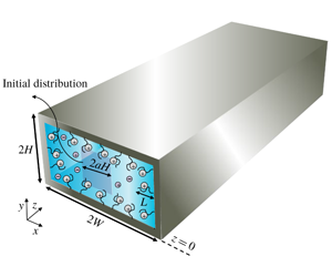
Consideration is given to the unsteady dispersion of a solute band by electroosmotic flow of a Newtonian liquid with constant physical properties in a straight rectangular microchannel with PEL-grafted walls. The channel dimensions, the coordinate system, located at the centre of the $X$–$Y$ plane at the channel entrance and other details are given in figure 1. It is assumed that the flow is both steady and fully developed. The probable adsorption/reaction of the solutes at the channel walls is accounted for via applying an irreversible first-order boundary reaction formula. The PEL is considered to have a constant and uniform charge density and a uniform thickness all around the channel with a sufficiently low grafting density to allow the use of the same values of permittivity and viscosity inside and outside the PEL. Since a low grafting density is considered, the volumetric density of the PEL fixed charges may be assumed to be low enough to permit application of the Debye–Hückel linearization when treating the problem analytically. It is further assumed that the Debye length is larger than the hydraulic diameter of the channel so that the concentration polarization effect arising due to the selective transport of ionic species can be ignored. Finally, the liquid is considered to contain an electrolyte of a completely dissociated symmetric salt. Owing to the symmetry, the analysis is limited to the first quarter of the channel.

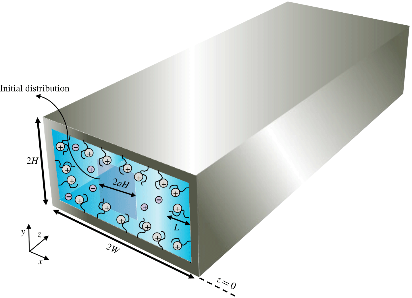
Figure 1. Schematic representation of the rectangular microchannel under consideration. The internal surface of the microchannel is coated with a polyelectrolyte layer of thickness $L$. The square of side length $2aH$ shows the shape of the initial solute distribution that is considered in the presentation of results.

2.2 Electric potential field

The overall electric potential field $\unicode[STIX]{x1D6F7}(X,Y,Z)$ within the microchannel is the superposition of the externally applied electric potential $\unicode[STIX]{x1D711}(Z)$ and the EDL electric potential $\unicode[STIX]{x1D6F9}(X,Y)$, that is

(2.1)$$\begin{eqnarray}\unicode[STIX]{x1D6F7}(X,Y,Z)=\unicode[STIX]{x1D6F9}(X,Y)+\unicode[STIX]{x1D711}(Z).\end{eqnarray}$$

The electric potential is governed by the Poisson equation, written as

(2.2)$$\begin{eqnarray}\unicode[STIX]{x1D6FB}^{2}\unicode[STIX]{x1D6F7}=-\frac{\unicode[STIX]{x1D70C}_{e}}{\unicode[STIX]{x1D700}},\end{eqnarray}$$

where $\unicode[STIX]{x1D700}$ represents the permittivity and $\unicode[STIX]{x1D70C}_{e}$ stands for the net electric charge density. As noted before, the same permittivities are assumed within and outside of the PEL. However, attention should be given to the fact that, since the permittivity of polyelectrolyte brushes is lower than that of water, the PEL permittivity is generally lower than solution permittivity. In fact, the range 52.8–78 is reported for the relative permittivity of the PEL (Sadeghi, Azari & Hardt Reference Sadeghi, Azari and Hardt2019). Whereas the lower limit differs significantly from water permittivity, the upper limit is quite close to it. This corresponds to the cases for which the grafting density is low, similar to the circumstances considered in the present study.

There are two types of electric charge in the microchannel, namely solution ions, which move freely throughout the whole domain under consideration, and PEL charges that are fixed within this layer. The net electric charges of solution and PEL ions are respectively given as

(2.3)$$\begin{eqnarray}\displaystyle \unicode[STIX]{x1D70C}_{E} & = & \displaystyle ez_{E}(C_{+}-C_{-})=ez_{E}C^{\infty }\left[\exp \left(-\frac{ez_{E}\unicode[STIX]{x1D6F9}}{k_{B}T}\right)-\exp \left(\frac{ez_{E}\unicode[STIX]{x1D6F9}}{k_{B}T}\right)\right]\nonumber\\ \displaystyle & = & \displaystyle -2ez_{E}C^{\infty }\sinh \left(\frac{ez_{E}\unicode[STIX]{x1D6F9}}{k_{B}T}\right),\end{eqnarray}$$

(2.4)$$\begin{eqnarray}\unicode[STIX]{x1D70C}_{PEL}=e\mathbb{N}_{PEL}z_{PEL},\end{eqnarray}$$

where $e$ is the proton charge, $K_{B}$ shows the Boltzmann constant, $T$ indicates the absolute temperature, $z_{E}$ denote the valence of electrolyte ions and $\mathbb{N}_{PEL}$ and $z_{PEL}$ are the number density and valence of the PEL fixed charges, respectively. In addition, $C_{+}$ and $C_{-}$ stand for the number concentrations of cations and anions, respectively, which both equal $C^{\infty }$ at neutral conditions. Note that a Boltzmann distribution is assumed for the solution ions since the fluid velocity does not influence the ionic distribution in the normal direction to a rectilinear flow. Substituting (2.3) and (2.4) into (2.2) and recalling that $\unicode[STIX]{x1D6FB}^{2}\unicode[STIX]{x1D711}=0$ for a constant applied electric field, one obtains

(2.5)$$\begin{eqnarray}\frac{\unicode[STIX]{x2202}^{2}\unicode[STIX]{x1D6F9}}{\unicode[STIX]{x2202}X^{2}}+\frac{\unicode[STIX]{x2202}^{2}\unicode[STIX]{x1D6F9}}{\unicode[STIX]{x2202}Y^{2}}-\frac{2ez_{E}C^{\infty }}{\unicode[STIX]{x1D700}}\sinh \left(\frac{ez_{E}\unicode[STIX]{x1D6F9}}{k_{B}T}\right)+\frac{e\mathbb{N}z_{PEL}}{\unicode[STIX]{x1D700}}=0.\end{eqnarray}$$

The parameter $\mathbb{N}$ appearing in (2.5), which is equal to $\mathbb{N}_{PEL}$ and 0 inside and outside of the grafted layer, respectively, reminds us of the fact that the existence of the fixed charges is limited to the PEL. It should be pointed out that the spatial distribution of the PEL fixed charges is generally non-uniform, with a decreasing dependence on the normal distance from the hard wall; however, depending on the properties of the electrolyte and brushes, situations may be found in which a uniform charge distribution, considered in this study, is reasonable (Sadeghi et al. Reference Sadeghi, Azari and Hardt2019). For low grafting densities, the electric potential is so low that the term $\sinh (ez_{E}\unicode[STIX]{x1D6F9}/k_{B}T)$ can be approximated by $ez_{E}\unicode[STIX]{x1D6F9}/k_{B}T$. This approximation, known as Debye–Hückel linearization, modifies equation (2.5) as

(2.6)$$\begin{eqnarray}\frac{\unicode[STIX]{x2202}^{2}\unicode[STIX]{x1D6F9}}{\unicode[STIX]{x2202}X^{2}}+\frac{\unicode[STIX]{x2202}^{2}\unicode[STIX]{x1D6F9}}{\unicode[STIX]{x2202}Y^{2}}-2\left(\frac{e^{2}z_{E}^{2}C^{\infty }}{k_{B}T\unicode[STIX]{x1D700}}\unicode[STIX]{x1D6F9}\right)+\frac{e\mathbb{N}z_{PEL}}{\unicode[STIX]{x1D700}}=0.\end{eqnarray}$$

By introducing the dimensionless parameters as below,

(2.7a-f)$$\begin{eqnarray}x=\frac{X}{H},\quad y=\frac{Y}{H},\quad \unicode[STIX]{x1D713}=\frac{ez_{E}\unicode[STIX]{x1D6F9}}{k_{B}T},\quad \mathbb{N}^{\ast }=\frac{\mathbb{N}}{\mathbb{N}_{PEL}},\quad K=H/\unicode[STIX]{x1D706}_{E},\quad \unicode[STIX]{x1D702}_{\unicode[STIX]{x1D706}}=\unicode[STIX]{x1D706}_{PEL}/\unicode[STIX]{x1D706}_{E},\end{eqnarray}$$

with $\unicode[STIX]{x1D706}_{E}=(k_{B}T\unicode[STIX]{x1D700}/2C^{\infty }e^{2}z_{E}^{2})^{1/2}$ and $\unicode[STIX]{x1D706}_{PEL}=(k_{B}T\unicode[STIX]{x1D700}/z_{E}z_{PEL}\mathbb{N}_{PEL}e^{2})^{1/2}$ being the characteristic and PEL Debye lengths, respectively, equation (2.6) is scaled as

(2.8)$$\begin{eqnarray}\frac{\unicode[STIX]{x2202}^{2}\unicode[STIX]{x1D713}}{\unicode[STIX]{x2202}x^{2}}+\frac{\unicode[STIX]{x2202}^{2}\unicode[STIX]{x1D713}}{\unicode[STIX]{x2202}y^{2}}-K^{2}\unicode[STIX]{x1D713}+K^{2}\unicode[STIX]{x1D702}_{\unicode[STIX]{x1D706}}^{-2}\mathbb{N}^{\ast }=0.\end{eqnarray}$$

The boundary conditions associated with (2.8) include

(2.9)$$\begin{eqnarray}\left.\frac{\unicode[STIX]{x2202}\unicode[STIX]{x1D713}}{\unicode[STIX]{x2202}x}\right|_{x=0}=\left.\frac{\unicode[STIX]{x2202}\unicode[STIX]{x1D713}}{\unicode[STIX]{x2202}x}\right|_{x=w}=\left.\frac{\unicode[STIX]{x2202}\unicode[STIX]{x1D713}}{\unicode[STIX]{x2202}y}\right|_{y=0}=\left.\frac{\unicode[STIX]{x2202}\unicode[STIX]{x1D713}}{\unicode[STIX]{x2202}y}\right|_{y=1}=0,\end{eqnarray}$$

where $w=W/H$. The boundary conditions (2.9) reflect symmetry at the centrelines and the neutrality of the rigid walls of the microchannel. Since the electrical potential and its gradient are continuous at the electrolyte–PEL interface, we consider for both domains a single solution of the form

(2.10)$$\begin{eqnarray}\unicode[STIX]{x1D713}=\mathop{\sum }_{j=1}^{\infty }b_{j}\cos (\unicode[STIX]{x1D709}_{l_{j}}y)\cos (\unicode[STIX]{x1D709}_{m_{j}}x/w),\end{eqnarray}$$

where $\unicode[STIX]{x1D709}_{l_{j}}=l_{j}\unicode[STIX]{x03C0}$ and $\unicode[STIX]{x1D709}_{m_{j}}=m_{j}\unicode[STIX]{x03C0}$ with $l_{j}=0,1,2,\ldots$ and $m_{j}=0,1,2,\ldots$ . The form (2.10) satisfies the pertinent boundary conditions. Substituting this functional form into (2.8) results in

(2.11)$$\begin{eqnarray}\mathop{\sum }_{j=1}^{\infty }b_{j}(\unicode[STIX]{x1D709}_{l_{j}}^{2}+\unicode[STIX]{x1D709}_{m_{j}}^{2}/w^{2}+K^{2})\cos (\unicode[STIX]{x1D709}_{l_{j}}y)\cos (\unicode[STIX]{x1D709}_{m_{j}}x/w)=K^{2}\unicode[STIX]{x1D702}_{\unicode[STIX]{x1D706}}^{-2}\mathbb{N}^{\ast }.\end{eqnarray}$$

Multiplying both sides of (2.11) by $\cos (\unicode[STIX]{x1D709}_{l_{i}}y)\cos (\unicode[STIX]{x1D709}_{m_{i}}x/w)$, integrating over the dimensionless cross-sectional area and making use of the orthogonality conditions, we obtain

(2.12)$$\begin{eqnarray}\displaystyle & & \displaystyle b_{i}(\unicode[STIX]{x1D709}_{l_{i}}^{2}+\unicode[STIX]{x1D709}_{m_{i}}^{2}/w^{2}+K^{2})\int _{0}^{w}\int _{0}^{1}\cos ^{2}(\unicode[STIX]{x1D709}_{l_{i}}y)\cos ^{2}(\unicode[STIX]{x1D709}_{m_{i}}x/w)\,\text{d}y\,\text{d}x\nonumber\\ \displaystyle & & \displaystyle \quad =K^{2}\unicode[STIX]{x1D702}_{\unicode[STIX]{x1D706}}^{-2}\int _{0}^{w}\int _{0}^{1}\mathbb{N}^{\ast }\cos (\unicode[STIX]{x1D709}_{l_{i}}y)\cos (\unicode[STIX]{x1D709}_{m_{i}}x/w)\,\text{d}y\,\text{d}x.\end{eqnarray}$$

Performing the integrations, $b_{i}$ is obtained as $b_{i}=c_{i}/a_{i}$ where

(2.13a)$$\begin{eqnarray}\displaystyle c_{i} & = & \displaystyle K^{2}\unicode[STIX]{x1D702}_{\unicode[STIX]{x1D706}}^{-2}w\left.\unicode[STIX]{x27E6}\unicode[STIX]{x1D6FF}_{0,l_{i}+m_{i}}-\left\{\unicode[STIX]{x1D6FF}_{0,l_{i}}(1-l)+(1-\unicode[STIX]{x1D6FF}_{0,l_{i}})\frac{\sin [\unicode[STIX]{x1D709}_{l_{i}}(1-l)]}{\unicode[STIX]{x1D709}_{l_{i}}}\right\}\left\{\unicode[STIX]{x1D6FF}_{0,m_{i}}(1-l/w)\right.\right.\nonumber\\ \displaystyle & & \displaystyle +\left.\left.(1-\unicode[STIX]{x1D6FF}_{0,m_{i}})\frac{\sin [\unicode[STIX]{x1D709}_{m_{i}}(1-l/w)]}{\unicode[STIX]{x1D709}_{m_{i}}}\right\}\right.\unicode[STIX]{x27E7},\end{eqnarray}$$

(2.13b)$$\begin{eqnarray}a_{i}=\frac{1}{4w}[w^{2}\unicode[STIX]{x1D709}_{l_{i}}^{2}(1+\unicode[STIX]{x1D6FF}_{0,m_{i}})+\unicode[STIX]{x1D709}_{m_{i}}^{2}(1+\unicode[STIX]{x1D6FF}_{0,l_{i}})+K^{2}w^{2}(1+\unicode[STIX]{x1D6FF}_{0,m_{i}})(1+\unicode[STIX]{x1D6FF}_{0,l_{i}})],\end{eqnarray}$$

where $\unicode[STIX]{x1D6FF}$ denotes the Kronecker delta and $l=L/H$ is the dimensionless thickness of the grafted layer.

2.2.1 Special solution for $w\rightarrow \infty$

When the channel aspect ratio is very large, that is for $1\ll w$, the dependence of the physical parameters on the $x$-coordinate vanishes. The solutions obtained under these circumstances are computationally less expensive and are more appropriate to experimentalists. The electric potential distribution for this case is found by solving the following ordinary differential equations for outside and inside the PEL, respectively,

(2.14)$$\begin{eqnarray}\displaystyle & \displaystyle \frac{\text{d}^{2}\unicode[STIX]{x1D713}_{E}}{\text{d}y^{2}}-K^{2}\unicode[STIX]{x1D713}_{E}=0, & \displaystyle\end{eqnarray}$$

(2.15)$$\begin{eqnarray}\displaystyle & \displaystyle \frac{\text{d}^{2}\unicode[STIX]{x1D713}_{PEL}}{\text{d}y^{2}}-K^{2}\unicode[STIX]{x1D713}_{PEL}+K^{2}\unicode[STIX]{x1D702}_{\unicode[STIX]{x1D706}}^{-2}=0, & \displaystyle\end{eqnarray}$$

which are subject to the following boundary and interfacial conditions:

(2.16a)$$\begin{eqnarray}\displaystyle & \displaystyle \left.\frac{\text{d}\unicode[STIX]{x1D713}_{E}}{\text{d}y}\right|_{y=0}=\left.\frac{\text{d}\unicode[STIX]{x1D713}_{PEL}}{\text{d}y}\right|_{y=1}=0, & \displaystyle\end{eqnarray}$$

(2.16b)$$\begin{eqnarray}\displaystyle & \displaystyle \left.\unicode[STIX]{x1D713}_{E}\right|_{y=1-l}=\left.\unicode[STIX]{x1D713}_{PEL}\right|_{y=1-l}, & \displaystyle\end{eqnarray}$$

(2.16c)$$\begin{eqnarray}\displaystyle & \displaystyle \left.\frac{\text{d}\unicode[STIX]{x1D713}_{E}}{\text{d}y}\right|_{y=1-l}=\left.\frac{\text{d}\unicode[STIX]{x1D713}_{PEL}}{\text{d}y}\right|_{y=1-l}. & \displaystyle\end{eqnarray}$$

It can be shown that the solutions of (2.14) and (2.15) subject to the pertinent boundary conditions are given as

(2.17)$$\begin{eqnarray}\displaystyle & \displaystyle \unicode[STIX]{x1D713}_{E}=b_{E1}\cosh (Ky), & \displaystyle\end{eqnarray}$$

(2.18)$$\begin{eqnarray}\displaystyle & \displaystyle \unicode[STIX]{x1D713}_{PEL}=b_{PEL1}[\cosh (Ky)-\tanh K\sinh (Ky)]+\unicode[STIX]{x1D702}_{\unicode[STIX]{x1D706}}^{-2}\unicode[STIX]{x1D6FE}^{-1}, & \displaystyle\end{eqnarray}$$

where

(2.19a)$$\begin{eqnarray}\displaystyle b_{E1} & = & \displaystyle \unicode[STIX]{x1D702}_{\unicode[STIX]{x1D706}}^{-2}\{\sinh [K(1-l)]\}^{-1}\{\!\tanh [K(1-l)]\nonumber\\ \displaystyle & & \displaystyle -\,\tanh K\!\}\unicode[STIX]{x27E6}\{\tanh [K(1-l)]\}^{-1}\{\tanh [K(1-l)]-\tanh K\}-1\nonumber\\ \displaystyle & & \displaystyle +\,\tanh K\tanh [K(1-l)]\unicode[STIX]{x27E7}^{-1},\end{eqnarray}$$

(2.19b)$$\begin{eqnarray}\displaystyle b_{PEL1} & = & \displaystyle \unicode[STIX]{x1D702}_{\unicode[STIX]{x1D706}}^{-2}\{\cosh [K(1-l)]\}^{-1}\unicode[STIX]{x27E6}\{\tanh [K(1-l)]\}^{-1}\{\tanh [K(1-l)]-\tanh K\}-1\nonumber\\ \displaystyle & & \displaystyle +\,\tanh K\tanh [K(1-l)]\unicode[STIX]{x27E7}^{-1}.\end{eqnarray}$$

2.3 Velocity distribution

For evaluation of the velocity field, the mathematical representation of the momentum conservation law must be solved. For an incompressible flow of Newtonian fluids with constant physical properties, the general form of the momentum equation reads

(2.20)$$\begin{eqnarray}\unicode[STIX]{x1D70C}\frac{\text{D}\boldsymbol{U}}{\text{D}t}=-\unicode[STIX]{x1D735}P+\unicode[STIX]{x1D707}\unicode[STIX]{x1D6FB}^{2}\boldsymbol{U}+\boldsymbol{F},\end{eqnarray}$$

where parameters $\unicode[STIX]{x1D70C}$, $t$, $\boldsymbol{U}$, $P$, $\unicode[STIX]{x1D707}$ and $\boldsymbol{F}$ denote the density, time, velocity vector, pressure, dynamic viscosity and body force vector, respectively. Since the flow is assumed to be both steady and fully developed, the inertia term is dropped from the momentum equation and the axial velocity $U_{z}$ becomes a function of the transverse coordinates only. The body force vector $\boldsymbol{F}$ is the superposition of the force exerted on the ions by the electric field $\boldsymbol{E}$, given as $\unicode[STIX]{x1D70C}_{e}\boldsymbol{E}$, and the drag force created by the polyelectrolyte brushes. The widely accepted approach to accounting for the drag force is to consider a volumetric resistive force proportional to the velocity, which is equivalent to modelling the PEL as a porous medium utilizing the Brinkman equation. For a fully developed flow, such a resistive force is given as $f_{PEL}U_{z}$ where $f_{PEL}$ is the friction coefficient of the PEL per unit volume. Adding the above-mentioned terms to the Navier–Stokes equation and substituting for $\unicode[STIX]{x1D70C}_{e}$ from (2.3) and (2.4), the momentum equation in the axial direction becomes

(2.21)$$\begin{eqnarray}\unicode[STIX]{x1D707}\left(\frac{\unicode[STIX]{x2202}^{2}U_{z}}{\unicode[STIX]{x2202}X^{2}}+\frac{\unicode[STIX]{x2202}^{2}U_{z}}{\unicode[STIX]{x2202}Y^{2}}\right)-fU_{z}-2ez_{E}E_{z}C^{\infty }\sinh \left(\frac{ez_{E}\unicode[STIX]{x1D713}}{k_{B}T}\right)=0,\end{eqnarray}$$

where $E_{z}$ is the applied electric field and the friction coefficient $f$ is equal to $f_{PEL}$ inside the grafted layer and 0 within the electrolyte. By introducing the following new dimensionless parameters

(2.22a-d)$$\begin{eqnarray}U_{0}=-\frac{\unicode[STIX]{x1D700}k_{B}TE_{z}}{ez_{E}\unicode[STIX]{x1D707}},\quad u=\frac{U_{z}}{U_{0}},\quad f^{\ast }=\frac{f}{f_{PEL}},\quad \unicode[STIX]{x1D6FC}=H\left(\frac{f_{PEL}}{\unicode[STIX]{x1D707}}\right)^{1/2},\end{eqnarray}$$

with $U_{0}=-\unicode[STIX]{x1D700}k_{B}TE_{z}/e\unicode[STIX]{x1D707}z_{E}$ being the reference velocity, and performing the Debye–Hückel linearization, the momentum equation (2.21) can be scaled as

(2.23)$$\begin{eqnarray}\frac{\unicode[STIX]{x2202}^{2}u}{\unicode[STIX]{x2202}x^{2}}+\frac{\unicode[STIX]{x2202}^{2}u}{\unicode[STIX]{x2202}y^{2}}-\unicode[STIX]{x1D6FC}^{2}f^{\ast }u+K^{2}\unicode[STIX]{x1D713}=0.\end{eqnarray}$$

The momentum equation is subject to symmetry and no-slip boundary conditions, which are written in dimensionless form as

(2.24)$$\begin{eqnarray}\left.\frac{\unicode[STIX]{x2202}u}{\unicode[STIX]{x2202}x}\right|_{x=0}=u|_{x=w}=\left.\frac{\unicode[STIX]{x2202}u}{\unicode[STIX]{x2202}y}\right|_{y=0}=u|_{y=1}=0.\end{eqnarray}$$

The solution of (2.23) satisfying the pertinent boundary conditions may be expressed as

(2.25)$$\begin{eqnarray}u=\mathop{\sum }_{j=1}^{\infty }d_{j}\cos (\unicode[STIX]{x1D709}_{r_{j}}y)\cos (\unicode[STIX]{x1D709}_{q_{j}}x/w),\end{eqnarray}$$

where $\unicode[STIX]{x1D709}_{r_{j}}=(2r_{j}+1)\unicode[STIX]{x03C0}/2$ and $\unicode[STIX]{x1D709}_{q_{j}}=(2q_{j}+1)\unicode[STIX]{x03C0}/2$ with $r_{j}=0,1,2,\ldots$ and $q_{j}=0,1,2,\ldots$ . Substituting the forms (2.10) and (2.25) into (2.23), multiplying both sides by $\cos (\unicode[STIX]{x1D709}_{r_{i}}y)\cos (\unicode[STIX]{x1D709}_{q_{i}}x/w)$ and integrating over the dimensionless cross-sectional area, one gets

(2.26)$$\begin{eqnarray}\displaystyle & & \displaystyle \mathop{\sum }_{j=1}^{\infty }d_{j}\int _{0}^{w}\int _{0}^{1}(\unicode[STIX]{x1D709}_{r_{j}}^{2}+\unicode[STIX]{x1D709}_{q_{j}}^{2}/w^{2}+\unicode[STIX]{x1D6FC}^{2}f^{\ast })\cos (\unicode[STIX]{x1D709}_{r_{i}}y)\cos (\unicode[STIX]{x1D709}_{q_{i}}x/w)\cos (\unicode[STIX]{x1D709}_{r_{j}}y)\cos (\unicode[STIX]{x1D709}_{q_{j}}x/w)\,\text{d}y\,\text{d}x\nonumber\\ \displaystyle & & \displaystyle \quad =K^{2}\mathop{\sum }_{j=1}^{\infty }b_{j}\int _{0}^{w}\int _{0}^{1}\cos (\unicode[STIX]{x1D709}_{r_{i}}y)\cos (\unicode[STIX]{x1D709}_{q_{i}}x/w)\cos (\unicode[STIX]{x1D709}_{l_{j}}y)\cos (\unicode[STIX]{x1D709}_{m_{j}}x/w)\,\text{d}y\,\text{d}x.\end{eqnarray}$$

It should be pointed out that, because of the position-dependent nature of $f^{\ast }$, the orthogonality condition does not hold for this case. Truncating the series on the left side from the $N$th term and that on the right side from the $M$th term and performing the integrations, a system of $N$ equations of $N$ unknowns including $d_{1},d_{2},\ldots ,d_{N}$ are obtained that may be written in matrix form as

(2.27)$$\begin{eqnarray}\unicode[STIX]{x1D640}\boldsymbol{d}=\boldsymbol{H},\end{eqnarray}$$

where the matrix $\unicode[STIX]{x1D640}$ and vector $\boldsymbol{H}$ have the following elements:

(2.28)$$\begin{eqnarray}\displaystyle e_{ij} & = & \displaystyle \frac{\unicode[STIX]{x1D6FF}_{r_{i},r_{j}}\unicode[STIX]{x1D6FF}_{q_{i},q_{j}}}{4w}(w^{2}\unicode[STIX]{x1D709}_{r_{i}}\unicode[STIX]{x1D709}_{r_{j}}+\unicode[STIX]{x1D709}_{q_{i}}\unicode[STIX]{x1D709}_{q_{j}})+\frac{\unicode[STIX]{x1D6FC}^{2}}{4}w\unicode[STIX]{x1D6FF}_{r_{i},r_{j}}\unicode[STIX]{x1D6FF}_{q_{i},q_{j}}\nonumber\\ \displaystyle & & \displaystyle -\,\frac{\unicode[STIX]{x1D6FC}^{2}w}{4}\left.\unicode[STIX]{x27E6}\unicode[STIX]{x1D6FF}_{r_{i},r_{j}}\left\{1-l+\frac{\sin [2\unicode[STIX]{x1D709}_{r_{i}}(1-l)]}{2\unicode[STIX]{x1D709}_{r_{i}}}\right\}\right.\nonumber\\ \displaystyle & & \displaystyle +\left.(1-\unicode[STIX]{x1D6FF}_{r_{i},r_{j}})\left\{\frac{\sin [(\unicode[STIX]{x1D709}_{r_{i}}-\unicode[STIX]{x1D709}_{r_{j}})(1-l)]}{\unicode[STIX]{x1D709}_{r_{i}}-\unicode[STIX]{x1D709}_{r_{j}}}-\frac{\sin [(\unicode[STIX]{x1D709}_{r_{i}}+\unicode[STIX]{x1D709}_{r_{j}})(1-l)]}{\unicode[STIX]{x1D709}_{r_{i}}+\unicode[STIX]{x1D709}_{r_{j}}}\right\}\right.\unicode[STIX]{x27E7}\left.\unicode[STIX]{x27E6}\unicode[STIX]{x1D6FF}_{q_{i},q_{j}}\left\{1-l/w\right.\right.\nonumber\\ \displaystyle & & \displaystyle +\left.\frac{\sin [2\unicode[STIX]{x1D709}_{q_{i}}(1-l/w)]}{2\unicode[STIX]{x1D709}_{q_{i}}}\right\}\nonumber\\ \displaystyle & & \displaystyle +\left.(1-\unicode[STIX]{x1D6FF}_{q_{i},q_{j}})\left\{\frac{\sin [(\unicode[STIX]{x1D709}_{q_{i}}-\unicode[STIX]{x1D709}_{q_{j}})(1-l/w)]}{\unicode[STIX]{x1D709}_{q_{i}}-\unicode[STIX]{x1D709}_{q_{j}}}+\frac{\sin [(\unicode[STIX]{x1D709}_{q_{i}}+\unicode[STIX]{x1D709}_{q_{j}})(1-l/w)]}{\unicode[STIX]{x1D709}_{q_{i}}+\unicode[STIX]{x1D709}_{q_{j}}}\right\}\right.\unicode[STIX]{x27E7},\end{eqnarray}$$

$$\begin{eqnarray}h_{i}=K^{2}\mathop{\sum }_{j=1}^{M}\frac{wb_{j}}{4}\left[\frac{(-1)^{r_{i}-l_{j}}}{\unicode[STIX]{x1D709}_{r_{i}}-\unicode[STIX]{x1D709}_{l_{j}}}+\frac{(-1)^{r_{i}+l_{j}}}{\unicode[STIX]{x1D709}_{r_{i}}+\unicode[STIX]{x1D709}_{l_{j}}}\right]\left[\frac{(-1)^{q_{i}-m_{j}}}{\unicode[STIX]{x1D709}_{q_{i}}-\unicode[STIX]{x1D709}_{m_{j}}}+\frac{(-1)^{q_{i}+m_{j}}}{\unicode[STIX]{x1D709}_{q_{i}}+\unicode[STIX]{x1D709}_{m_{j}}}\right].\end{eqnarray}$$

So the vector $\boldsymbol{d}$, which stands for the coefficients $d_{j}$, can be readily obtained as $\boldsymbol{d}=\unicode[STIX]{x1D640}^{-1}\boldsymbol{H}$.

As soon as the dimensionless velocity $u$ is obtained, the dimensionless mean velocity can be evaluated as

(2.29)$$\begin{eqnarray}u_{m}=\frac{\displaystyle \int _{0}^{w}\int _{0}^{1}u\,\text{d}y\,\text{d}x}{\displaystyle \int _{0}^{w}\int _{0}^{1}\,\text{d}y\,\text{d}x}=\mathop{\sum }_{j=1}^{N}\frac{d_{j}(-1)^{r_{j}+q_{j}}}{\unicode[STIX]{x1D709}_{r_{j}}\unicode[STIX]{x1D709}_{q_{j}}}.\end{eqnarray}$$

2.3.1 Special solution for $w\rightarrow \infty$

The momentum equation for this case reduces to the following equations for the electrolyte and the PEL:

(2.30)$$\begin{eqnarray}\displaystyle & \displaystyle \frac{\text{d}^{2}u_{E}}{\text{d}y^{2}}+K^{2}u_{E}=0, & \displaystyle\end{eqnarray}$$

(2.31)$$\begin{eqnarray}\displaystyle & \displaystyle \frac{\text{d}^{2}u_{PEL}}{\text{d}y^{2}}-\unicode[STIX]{x1D6FC}^{2}u_{PEL}+K^{2}\unicode[STIX]{x1D713}_{PEL}=0. & \displaystyle\end{eqnarray}$$

In addition, the boundary and interfacial conditions read

(2.32a)$$\begin{eqnarray}\displaystyle & \displaystyle \left.\frac{\text{d}u_{E}}{\text{d}y}\right|_{y=0}=u_{PEL}|_{y=1}=0, & \displaystyle\end{eqnarray}$$

(2.32b)$$\begin{eqnarray}\displaystyle & \displaystyle u_{E}|_{y=1-l}=u_{PEL}|_{y=1-l}, & \displaystyle\end{eqnarray}$$

(2.32c)$$\begin{eqnarray}\displaystyle & \displaystyle \left.\frac{\text{d}u_{E}}{\text{d}y}\right|_{y=1-l}=\left.\frac{\text{d}u_{PEL}}{\text{d}y}\right|_{y=1-l}. & \displaystyle\end{eqnarray}$$

It can be demonstrated that the solutions of (2.30) and (2.31) subject to the conditions (2.32) are given as

(2.33)$$\begin{eqnarray}u_{E}=-b_{E1}\cosh (Ky)+b_{E2},\end{eqnarray}$$

(2.34)$$\begin{eqnarray}\displaystyle u_{PEL} & = & \displaystyle b_{PEL2}[\cosh (\unicode[STIX]{x1D6FC}y)-\coth \unicode[STIX]{x1D6FC}\sinh (\unicode[STIX]{x1D6FC}y)]\nonumber\\ \displaystyle & & \displaystyle +\,\left[(\cosh K)^{-1}\left(\frac{K^{2}b_{PEL1}}{K^{2}-\unicode[STIX]{x1D6FC}^{2}}\right)-\frac{K^{2}}{\unicode[STIX]{x1D6FC}^{2}\unicode[STIX]{x1D702}_{\unicode[STIX]{x1D706}}^{2}}\right]\frac{\sinh (\unicode[STIX]{x1D6FC}y)}{\sinh \unicode[STIX]{x1D6FC}}\nonumber\\ \displaystyle & & \displaystyle -\,\left(\frac{K^{2}b_{PEL1}}{K^{2}-\unicode[STIX]{x1D6FC}^{2}}\right)\cosh (Ky)+\tanh K\left(\frac{K^{2}b_{PEL1}}{K^{2}-\unicode[STIX]{x1D6FC}^{2}}\right)\sinh (Ky)+\frac{K^{2}}{\unicode[STIX]{x1D6FC}^{2}\unicode[STIX]{x1D702}_{\unicode[STIX]{x1D706}}^{2}},\qquad\end{eqnarray}$$

where

(2.35a)$$\begin{eqnarray}\displaystyle & & \displaystyle b_{E2}=b_{PEL2}\{\cosh [\unicode[STIX]{x1D6FC}(1-l)]-\coth \unicode[STIX]{x1D6FC}\sinh [\unicode[STIX]{x1D6FC}(1-l)]\}\nonumber\\ \displaystyle & & \displaystyle \quad +\,\left[(\cosh K)^{-1}\left(\frac{K^{2}b_{PEL1}}{K^{2}-\unicode[STIX]{x1D6FC}^{2}}\right)-\frac{K^{2}}{\unicode[STIX]{x1D6FC}^{2}\unicode[STIX]{x1D702}_{\unicode[STIX]{x1D706}}^{2}}\right]\frac{\sinh [\unicode[STIX]{x1D6FC}(1-l)]}{\sinh \unicode[STIX]{x1D6FC}}-\left(\frac{K^{2}b_{PEL1}}{K^{2}-\unicode[STIX]{x1D6FC}^{2}}\right)\cosh [K(1-l)]\nonumber\\ \displaystyle & & \displaystyle \quad +\,\tanh K\left(\frac{K^{2}b_{PEL1}}{K^{2}-\unicode[STIX]{x1D6FC}^{2}}\right)\sinh [K(1-l)]+\frac{K^{2}}{\unicode[STIX]{x1D6FC}^{2}\unicode[STIX]{x1D702}_{\unicode[STIX]{x1D706}}^{2}}+b_{E1}\cosh [K(1-l)],\end{eqnarray}$$

(2.35b)$$\begin{eqnarray}\displaystyle b_{PEL2} & = & \displaystyle \unicode[STIX]{x1D6FC}^{-1}\{\sinh [\unicode[STIX]{x1D6FC}(1-l)]-\coth \unicode[STIX]{x1D6FC}\cosh [\unicode[STIX]{x1D6FC}(1-l)]\}^{-1}\left\{-b_{E1}K\sinh [K(1-l)]\right.\nonumber\\ \displaystyle & & \displaystyle -\,\unicode[STIX]{x1D6FC}\left[(\cosh K)^{-1}\left(\frac{K^{2}b_{PEL1}}{K^{2}-\unicode[STIX]{x1D6FC}^{2}}\right)-\frac{K^{2}}{\unicode[STIX]{x1D6FC}^{2}\unicode[STIX]{x1D702}_{\unicode[STIX]{x1D706}}^{2}}\right]\nonumber\\ \displaystyle & & \displaystyle \times \,\frac{\cosh [\unicode[STIX]{x1D6FC}(1-l)]}{\sinh \unicode[STIX]{x1D6FC}}+\left(\frac{K^{3}b_{PEL1}}{K^{2}-\unicode[STIX]{x1D6FC}^{2}}\right)\sinh [K(1-l)]\nonumber\\ \displaystyle & & \displaystyle -\left.\left(\frac{K^{3}b_{PEL1}}{K^{2}-\unicode[STIX]{x1D6FC}^{2}}\right)\tanh K\cosh [K(1-l)]\right\}.\end{eqnarray}$$

And the mean velocity becomes

(2.36)$$\begin{eqnarray}\displaystyle u_{m} & = & \displaystyle \int _{0}^{1-l}u_{E}\,\text{d}y+\int _{1-l}^{1}u_{PEL}\,\text{d}y\nonumber\\ \displaystyle & = & \displaystyle -\frac{b_{E1}}{K}\sinh [K(1-l)]+b_{E2}(1-l)\nonumber\\ \displaystyle & & \displaystyle -\,\unicode[STIX]{x1D6FC}^{-1}b_{PEL2}\{\sinh [\unicode[STIX]{x1D6FC}(1-l)]-\coth \unicode[STIX]{x1D6FC}\cosh [\unicode[STIX]{x1D6FC}(1-l)]+(\sinh \unicode[STIX]{x1D6FC})^{-1}\}\nonumber\\ \displaystyle & & \displaystyle +\,K^{2}\unicode[STIX]{x1D6FC}^{-1}\left[(\cosh K)^{-1}\left(\frac{b_{PEL1}}{K^{2}-\unicode[STIX]{x1D6FC}^{2}}\right)-\unicode[STIX]{x1D6FC}^{-2}\unicode[STIX]{x1D702}_{\unicode[STIX]{x1D706}}^{-2}\right]\left\{\coth \unicode[STIX]{x1D6FC}-\frac{\cosh [\unicode[STIX]{x1D6FC}(1-l)]}{\sinh \unicode[STIX]{x1D6FC}}\right\}\nonumber\\ \displaystyle & & \displaystyle -\,\left(\frac{Kb_{PEL1}}{K^{2}-\unicode[STIX]{x1D6FC}^{2}}\right)\{\sinh K-\sinh [K(1-l)]\}+\tanh K\left(\frac{Kb_{PEL1}}{K^{2}-\unicode[STIX]{x1D6FC}^{2}}\right)\nonumber\\ \displaystyle & & \displaystyle \times \,\{\cosh K-\cosh [K(1-l)]\}+\frac{K^{2}l}{\unicode[STIX]{x1D6FC}^{2}\unicode[STIX]{x1D702}_{\unicode[STIX]{x1D706}}^{2}}.\end{eqnarray}$$

2.4 Concentration field

The solute concentration distribution due to an injection source at $z=0$ can be described by the following transient advective–diffusive equation:

(2.37)$$\begin{eqnarray}\frac{\unicode[STIX]{x2202}C}{\unicode[STIX]{x2202}\unicode[STIX]{x1D70F}}+\unicode[STIX]{x1D735}\boldsymbol{\cdot }(\boldsymbol{U}C)=\unicode[STIX]{x1D735}\boldsymbol{\cdot }(D\unicode[STIX]{x1D735}C),\end{eqnarray}$$

where $\unicode[STIX]{x1D70F}$ denotes the time, $D$ stands for the molecular diffusivity and $C$ is the number concentration of solutes. Note that, due to the presence of polyelectrolyte brushes, the molecular diffusivity in the PEL is smaller than that in the bulk. Nevertheless, considering the fact that the effective diffusion coefficient in a porous medium of high porosity is approximately the same as that in void spaces (Vafai Reference Vafai2005), the diffusion coefficient in the soft layer may be considered the same as that in the bulk due to the small grafting densities assumed in the analysis. As we would like to perform separate analyses for slit and rectangular microchannels, the subscripts 1 and 2 are hereafter used for these geometries, respectively, to distinguish between the associated concentrations. Since we consider a fully developed flow of a liquid with constant thermophysical properties, equation (2.37) can be simplified to yield the following equations for slit and rectangular geometries, respectively,

(2.38)$$\begin{eqnarray}\displaystyle & \displaystyle \frac{\unicode[STIX]{x2202}C_{1}}{\unicode[STIX]{x2202}\unicode[STIX]{x1D70F}}+U_{z}\frac{\unicode[STIX]{x2202}C_{1}}{\unicode[STIX]{x2202}Z}=D\left[\frac{\unicode[STIX]{x2202}^{2}C_{1}}{\unicode[STIX]{x2202}Y^{2}}+\frac{\unicode[STIX]{x2202}^{2}C_{1}}{\unicode[STIX]{x2202}Z^{2}}\right], & \displaystyle\end{eqnarray}$$

(2.39)$$\begin{eqnarray}\displaystyle & \displaystyle \frac{\unicode[STIX]{x2202}C_{2}}{\unicode[STIX]{x2202}\unicode[STIX]{x1D70F}}+U_{z}\frac{\unicode[STIX]{x2202}C_{2}}{\unicode[STIX]{x2202}Z}=D\left[\frac{\unicode[STIX]{x2202}^{2}C_{2}}{\unicode[STIX]{x2202}X^{2}}+\frac{\unicode[STIX]{x2202}^{2}C_{2}}{\unicode[STIX]{x2202}Y^{2}}+\frac{\unicode[STIX]{x2202}^{2}C_{2}}{\unicode[STIX]{x2202}Z^{2}}\right], & \displaystyle\end{eqnarray}$$

which are subject to the following initial and boundary conditions:

(2.40a)$$\begin{eqnarray}\displaystyle & \displaystyle C_{1}(0,Y,Z)=C_{0}H\unicode[STIX]{x1D6FF}(Z)\unicode[STIX]{x1D703}_{1}(Y), & \displaystyle\end{eqnarray}$$

(2.40b)$$\begin{eqnarray}\displaystyle & \displaystyle \left.\frac{\unicode[STIX]{x2202}C_{1}}{\unicode[STIX]{x2202}Y}\right|_{Y=0}=\left.\frac{\unicode[STIX]{x2202}C_{1}}{\unicode[STIX]{x2202}X}\right|_{X=0}=0, & \displaystyle\end{eqnarray}$$

(2.40c)$$\begin{eqnarray}\displaystyle & \displaystyle -D\left.\frac{\unicode[STIX]{x2202}C_{1}}{\unicode[STIX]{x2202}Y}\right|_{Y=H}=k_{R}C_{1}|_{Y=H},\quad -D\left.\frac{\unicode[STIX]{x2202}C_{1}}{\unicode[STIX]{x2202}X}\right|_{X=W}=k_{R}C_{1}|_{X=W}, & \displaystyle\end{eqnarray}$$

(2.40d)$$\begin{eqnarray}\displaystyle & \displaystyle \lim _{Z\rightarrow \infty }C_{1}=\lim _{Z\rightarrow \infty }\frac{\unicode[STIX]{x2202}C_{1}}{\unicode[STIX]{x2202}Z}=0, & \displaystyle\end{eqnarray}$$

(2.41a)$$\begin{eqnarray}\displaystyle & \displaystyle C_{2}(0,X,Y,Z)=C_{0}H\unicode[STIX]{x1D6FF}(Z)\unicode[STIX]{x1D703}_{2}(X,Y), & \displaystyle\end{eqnarray}$$

(2.41b)$$\begin{eqnarray}\displaystyle & \displaystyle \left.\frac{\unicode[STIX]{x2202}C_{2}}{\unicode[STIX]{x2202}Y}\right|_{Y=0}=\left.\frac{\unicode[STIX]{x2202}C_{2}}{\unicode[STIX]{x2202}X}\right|_{X=0}=0, & \displaystyle\end{eqnarray}$$

(2.41c)$$\begin{eqnarray}\displaystyle & \displaystyle -D\left.\frac{\unicode[STIX]{x2202}C_{2}}{\unicode[STIX]{x2202}Y}\right|_{Y=H}=k_{R}C_{2}|_{Y=H},\quad -D\left.\frac{\unicode[STIX]{x2202}C_{2}}{\unicode[STIX]{x2202}X}\right|_{X=W}=k_{R}C_{2}|_{X=W}, & \displaystyle\end{eqnarray}$$

(2.41d)$$\begin{eqnarray}\displaystyle & \displaystyle \lim _{Z\rightarrow \infty }C_{2}=\lim _{Z\rightarrow \infty }\frac{\unicode[STIX]{x2202}C_{2}}{\unicode[STIX]{x2202}Z}=0, & \displaystyle\end{eqnarray}$$

where $\unicode[STIX]{x1D6FF}$ is the Dirac delta function. Equations (2.40c) and (2.41c) show that an irreversible first-order reaction with the rate $k_{R}$ occurs at the walls. It is here emphasized that, although irreversible reactions are possible in microfluidic devices, surface adsorption is mainly a reversible phenomenon, which is usually modelled by a first-order Langmuir adsorption model (Sadeghi et al. Reference Sadeghi, Amini, Saidi and Chakraborty2014). Approximating the Langmuir model by the form given in (2.40c) and (2.41c) is inevitable for analytical tractability of the problem. This way, we neglect some characteristics of reversible surface reactions, while retaining its most important physical features that are the same as those for reversible reactions.

Equations (2.38) and (2.39) are made dimensionless by using the following dimensionless parameters:

(2.42a-e)$$\begin{eqnarray}c_{i}=\frac{C_{i}}{C_{0}},\quad t=\frac{\unicode[STIX]{x1D70F}D}{H^{2}},\quad z=\frac{Z}{HPe},\quad Pe=\frac{HU_{0}}{D},\quad Da=\frac{Hk_{R}}{D}.\end{eqnarray}$$

The dimensionless solute transport equations and the pertinent initial and boundary conditions then become

(2.43)$$\begin{eqnarray}\frac{\unicode[STIX]{x2202}c_{1}}{\unicode[STIX]{x2202}t}+u_{1}(y)\frac{\unicode[STIX]{x2202}c_{1}}{\unicode[STIX]{x2202}z}=\frac{\unicode[STIX]{x2202}^{2}c_{1}}{\unicode[STIX]{x2202}y^{2}}+\frac{1}{Pe^{2}}\frac{\unicode[STIX]{x2202}^{2}c_{1}}{\unicode[STIX]{x2202}z^{2}},\end{eqnarray}$$

(2.44a)$$\begin{eqnarray}\displaystyle & \displaystyle c_{1}(0,y,z)=Pe^{-1}\unicode[STIX]{x1D6FF}(z)\unicode[STIX]{x1D703}_{1}(y), & \displaystyle\end{eqnarray}$$

(2.44b)$$\begin{eqnarray}\displaystyle & \displaystyle \left.\frac{\unicode[STIX]{x2202}c_{1}}{\unicode[STIX]{x2202}y}\right|_{y=0}=0, & \displaystyle\end{eqnarray}$$

(2.44c)$$\begin{eqnarray}\displaystyle & \displaystyle \left.\frac{\unicode[STIX]{x2202}c_{1}}{\unicode[STIX]{x2202}y}\right|_{y=1}=-Dac_{1}|_{y=1}, & \displaystyle\end{eqnarray}$$

(2.44d)$$\begin{eqnarray}\displaystyle & \displaystyle \lim _{z\rightarrow \infty }c_{1}=\lim _{z\rightarrow \infty }\frac{\unicode[STIX]{x2202}c_{1}}{\unicode[STIX]{x2202}z}=0, & \displaystyle\end{eqnarray}$$

(2.45)$$\begin{eqnarray}\frac{\unicode[STIX]{x2202}c_{2}}{\unicode[STIX]{x2202}t}+u_{2}(x,y)\frac{\unicode[STIX]{x2202}c_{2}}{\unicode[STIX]{x2202}z}=\frac{\unicode[STIX]{x2202}^{2}c_{2}}{\unicode[STIX]{x2202}x^{2}}+\frac{\unicode[STIX]{x2202}^{2}c_{2}}{\unicode[STIX]{x2202}y^{2}}+\frac{1}{Pe^{2}}\frac{\unicode[STIX]{x2202}^{2}c_{2}}{\unicode[STIX]{x2202}z^{2}},\end{eqnarray}$$

(2.46a)$$\begin{eqnarray}\displaystyle & \displaystyle c_{2}(0,x,y,z)=Pe^{-1}\unicode[STIX]{x1D6FF}(z)\unicode[STIX]{x1D703}_{2}(x,y), & \displaystyle\end{eqnarray}$$

(2.46b)$$\begin{eqnarray}\displaystyle & \displaystyle \left.\frac{\unicode[STIX]{x2202}c_{2}}{\unicode[STIX]{x2202}y}\right|_{y=0}=\left.\frac{\unicode[STIX]{x2202}c_{2}}{\unicode[STIX]{x2202}x}\right|_{x=0}=0, & \displaystyle\end{eqnarray}$$

(2.46c)$$\begin{eqnarray}\displaystyle & \displaystyle \left.\frac{\unicode[STIX]{x2202}c_{2}}{\unicode[STIX]{x2202}y}\right|_{y=1}=-Dac_{2}|_{y=1},\quad \left.\frac{\unicode[STIX]{x2202}c_{2}}{\unicode[STIX]{x2202}x}\right|_{x=w}=-Dac_{2}|_{x=w}, & \displaystyle\end{eqnarray}$$

(2.46d)$$\begin{eqnarray}\displaystyle & \displaystyle \lim _{z\rightarrow \infty }c_{2}=\lim _{z\rightarrow \infty }\frac{\unicode[STIX]{x2202}c_{2}}{\unicode[STIX]{x2202}z}=0. & \displaystyle\end{eqnarray}$$

The unsteady transport equation with the associated initial and boundary conditions can be solved using the method proposed by Gill & Sankarasubramanian (Reference Gill and Sankarasubramanian1970). In this method, the solute concentration $c$ is expanded in an infinite series as follows:

(2.47)$$\begin{eqnarray}\displaystyle & \displaystyle c_{1}(t,y,z)=\mathop{\sum }_{n=0}^{\infty }f_{n,1}(t,y)\frac{\unicode[STIX]{x2202}^{n}c_{m,1}(t,z)}{\unicode[STIX]{x2202}z^{n}}, & \displaystyle\end{eqnarray}$$

(2.48)$$\begin{eqnarray}\displaystyle & \displaystyle c_{2}(t,x,y,z)=\mathop{\sum }_{n=0}^{\infty }f_{n,2}(t,x,y)\frac{\unicode[STIX]{x2202}^{n}c_{m,2}(t,z)}{\unicode[STIX]{x2202}z^{n}}, & \displaystyle\end{eqnarray}$$

where the dimensionless mean concentration $c_{m}(t,z)$ is defined as

(2.49)$$\begin{eqnarray}\displaystyle & \displaystyle c_{m,1}(t,z)=\int _{0}^{1}c_{1}\,\text{d}y, & \displaystyle\end{eqnarray}$$

(2.50)$$\begin{eqnarray}\displaystyle & \displaystyle c_{m,2}(t,z)=\frac{\displaystyle \int _{0}^{w}\int _{0}^{1}c_{2}\,\text{d}y\,\text{d}x}{w}. & \displaystyle\end{eqnarray}$$

By integrating the dimensionless concentration equations (2.43) and (2.45) over the microchannel cross-sectional area and using the mean concentration definition in (2.49) and (2.50) we will have

(2.51)$$\begin{eqnarray}\frac{\unicode[STIX]{x2202}c_{m,1}}{\unicode[STIX]{x2202}t}=\frac{1}{Pe^{2}}\frac{\unicode[STIX]{x2202}^{2}c_{m,1}}{\unicode[STIX]{x2202}z^{2}}+\left.\frac{\unicode[STIX]{x2202}c_{1}}{\unicode[STIX]{x2202}y}\right|_{y=1}-\frac{\unicode[STIX]{x2202}}{\unicode[STIX]{x2202}z}\int _{0}^{1}u_{1}c_{1}\,\text{d}y,\end{eqnarray}$$

(2.52)$$\begin{eqnarray}\displaystyle \frac{\unicode[STIX]{x2202}c_{m,2}}{\unicode[STIX]{x2202}t} & = & \displaystyle \frac{1}{Pe^{2}}\frac{\unicode[STIX]{x2202}^{2}c_{m,2}}{\unicode[STIX]{x2202}z^{2}}+\frac{1}{w}\left(\int _{0}^{1}\left.\frac{\unicode[STIX]{x2202}c_{2}}{\unicode[STIX]{x2202}x}\right|_{x=w}\,\text{d}y+\int _{0}^{w}\left.\frac{\unicode[STIX]{x2202}c_{2}}{\unicode[STIX]{x2202}y}\right|_{y=1}\,\text{d}x\right)\nonumber\\ \displaystyle & & \displaystyle -\,\frac{1}{w}\frac{\unicode[STIX]{x2202}}{\unicode[STIX]{x2202}z}\int _{0}^{1}\int _{0}^{w}u_{2}c_{2}\,\text{d}x\,\text{d}y.\end{eqnarray}$$

Then, substituting the local concentration formulas from (2.47) and (2.48) into (2.51) and (2.52) and rearranging gives the following dispersion model for $c_{m}$:

(2.53)$$\begin{eqnarray}\frac{\unicode[STIX]{x2202}c_{m,i}}{\unicode[STIX]{x2202}t}=\mathop{\sum }_{n=0}^{\infty }K_{n,i}(t)\frac{\unicode[STIX]{x2202}^{n}c_{m,i}(t,z)}{\unicode[STIX]{x2202}z^{n}},\quad i=1,2,\end{eqnarray}$$

where the coefficients $K_{n,i}(t)$ are

(2.54)$$\begin{eqnarray}K_{n,1}(t)=\frac{\unicode[STIX]{x1D6FF}_{n,2}}{Pe^{2}}+\left.\frac{\unicode[STIX]{x2202}f_{n,1}}{\unicode[STIX]{x2202}y}\right|_{y=1}-\int _{0}^{1}u_{1}(y)f_{n-1,1}\,\text{d}y,\quad n=0,1,2,\ldots ,\end{eqnarray}$$

(2.55)$$\begin{eqnarray}\displaystyle K_{n,2}(t) & = & \displaystyle \frac{\unicode[STIX]{x1D6FF}_{n,2}}{Pe^{2}}+\frac{1}{w}\left(\int _{0}^{1}\left.\frac{\unicode[STIX]{x2202}f_{n,2}}{\unicode[STIX]{x2202}x}\right|_{x=w}\,\text{d}y+\int _{0}^{w}\left.\frac{\unicode[STIX]{x2202}f_{n,2}}{\unicode[STIX]{x2202}y}\right|_{y=1}\,\text{d}x\right)\nonumber\\ \displaystyle & & \displaystyle -\,\frac{1}{w}\int _{0}^{1}\int _{0}^{w}u_{2}(x,y)f_{n-1,2}\,\text{d}x\,\text{d}y,\quad n=0,1,2\ldots .\end{eqnarray}$$

Neglecting the terms with $3\leqslant n$ due to their negligible contribution to the dispersion of the mean concentration, equation (2.53) is reduced to

(2.56)$$\begin{eqnarray}\frac{\unicode[STIX]{x2202}c_{m,i}}{\unicode[STIX]{x2202}t}=K_{0,i}(t)c_{m,i}+K_{1,i}(t)\frac{\unicode[STIX]{x2202}c_{m,i}}{\unicode[STIX]{x2202}z}+K_{2,i}(t)\frac{\unicode[STIX]{x2202}^{2}c_{m,i}}{\unicode[STIX]{x2202}z^{2}},\end{eqnarray}$$

where $K_{0,i}(t)$ is the exchange coefficient due to non-zero solute flux at the tube wall, $K_{1,i}(t)$ is the convection coefficient due to convective transport of the solutes and $K_{2,i}(t)$ is the dispersion coefficient due to molecular diffusion and non-uniformity of the velocity profile. So the behaviour of solute dispersion can be described well by evaluating these three transport coefficients.

Besides appropriate initial and boundary conditions, the determination of $K_{0,i}(t)$, $K_{1,i}(t)$ and $K_{2,i}(t)$ is needed to solve (2.56). Considering (2.54) and (2.55), we must first evaluate functions $f_{n}$. The equations governing $f_{n}$ can be achieved by substituting the local concentration distributions from (2.47) and (2.48) and also the time derivative of $c_{m}$ from (2.53) into (2.43) and (2.45) and then equating the coefficients of $\unicode[STIX]{x2202}^{n}c_{m}/\unicode[STIX]{x2202}z^{n}$. The desired equations then read

(2.57)$$\begin{eqnarray}\displaystyle & \displaystyle \frac{\unicode[STIX]{x2202}f_{n,1}}{\unicode[STIX]{x2202}t}=\frac{\unicode[STIX]{x2202}^{2}f_{n,1}}{\unicode[STIX]{x2202}y^{2}}+\frac{f_{n-2,1}}{Pe^{2}}-u_{1}f_{n-1,1}-\mathop{\sum }_{i=0}^{\infty }f_{n-i,1}K_{i,1}(t), & \displaystyle\end{eqnarray}$$

(2.58)$$\begin{eqnarray}\displaystyle & \displaystyle \frac{\unicode[STIX]{x2202}f_{n,2}}{\unicode[STIX]{x2202}t}=\frac{\unicode[STIX]{x2202}^{2}f_{n,2}}{\unicode[STIX]{x2202}x^{2}}+\frac{\unicode[STIX]{x2202}^{2}f_{n,2}}{\unicode[STIX]{x2202}y^{2}}+\frac{f_{n-2,2}}{Pe^{2}}-u_{2}f_{n-1,2}-\mathop{\sum }_{i=0}^{\infty }f_{n-i,2}K_{i,2}(t), & \displaystyle\end{eqnarray}$$

where $f_{-1}=f_{-2}=\cdots =0$. Substituting (2.47) and (2.48) into (2.44) and (2.46) and recalling that $c_{m,i}(0,z)=Pe^{-1}\unicode[STIX]{x1D6FF}(z)\unicode[STIX]{x1D703}_{m,i}$ where $\unicode[STIX]{x1D703}_{m,1}=\int _{0}^{1}\unicode[STIX]{x1D703}_{1}\,\text{d}y$ and $\unicode[STIX]{x1D703}_{m,2}=\int _{0}^{1}\int _{0}^{w}\unicode[STIX]{x1D703}_{2}\,\text{d}x\,\text{d}y/w$, the associated initial and boundary conditions are obtained as

(2.59a)$$\begin{eqnarray}\displaystyle & \displaystyle f_{0,1}(0,y)=\frac{\unicode[STIX]{x1D703}_{1}(y)}{\unicode[STIX]{x1D703}_{m,1}},\quad f_{n\geqslant 1,1}(0,y)=0, & \displaystyle\end{eqnarray}$$

(2.59b)$$\begin{eqnarray}\displaystyle & \displaystyle \left.\frac{\unicode[STIX]{x2202}f_{n,1}}{\unicode[STIX]{x2202}y}\right|_{y=0}=0, & \displaystyle\end{eqnarray}$$

(2.59c)$$\begin{eqnarray}\displaystyle & \displaystyle \left.\frac{\unicode[STIX]{x2202}f_{n,1}}{\unicode[STIX]{x2202}y}\right|_{y=1}=-Daf_{n,1}|_{y=1}, & \displaystyle\end{eqnarray}$$

(2.60a)$$\begin{eqnarray}\displaystyle & \displaystyle f_{0,2}(0,x,y)=\frac{\unicode[STIX]{x1D703}_{2}(x,y)}{\unicode[STIX]{x1D703}_{m,2}},\quad f_{n\geqslant 1,2}(0,x,y)=0, & \displaystyle\end{eqnarray}$$

(2.60b)$$\begin{eqnarray}\displaystyle & \displaystyle \left.\frac{\unicode[STIX]{x2202}f_{n,2}}{\unicode[STIX]{x2202}x}\right|_{x=0}=\left.\frac{\unicode[STIX]{x2202}f_{n,2}}{\unicode[STIX]{x2202}y}\right|_{y=0}=0, & \displaystyle\end{eqnarray}$$

(2.60c)$$\begin{eqnarray}\displaystyle & \displaystyle \left.\frac{\unicode[STIX]{x2202}f_{n,2}}{\unicode[STIX]{x2202}x}\right|_{x=w}=-Daf_{n,2}|_{x=w},\quad \left.\frac{\unicode[STIX]{x2202}f_{n,2}}{\unicode[STIX]{x2202}y}\right|_{y=1}=-Daf_{n,2}|_{y=1}. & \displaystyle\end{eqnarray}$$

Now, integrating (2.59a) and (2.60a) over the dimensionless cross-sectional area provides

(2.61)$$\begin{eqnarray}\displaystyle & \displaystyle \int _{0}^{1}f_{n,1}\,\text{d}y=\unicode[STIX]{x1D6FF}_{n,0}, & \displaystyle\end{eqnarray}$$

(2.62)$$\begin{eqnarray}\displaystyle & \displaystyle \frac{1}{w}\int _{0}^{w}\int _{0}^{1}f_{n,2}\,\text{d}y\,\text{d}x=\unicode[STIX]{x1D6FF}_{n,0}. & \displaystyle\end{eqnarray}$$

In order to obtain the unsteady solution transport in the microchannel, the unknown parameters $K_{0,i}(t)$, $K_{1,i}(t)$, $K_{2,i}(t)$ and $f_{0,i}(t,x,y)$, $f_{1,i}(t,x,y)$ and $f_{2,i}(t,x,y)$ must be evaluated via solving the coupled systems of (2.57) and (2.58) subject to the associated boundary conditions given in (2.59) and (2.60). An appropriate method is to utilize the eigenfunction expansion, a method that is adopted here.

2.4.1 Exchange coefficient

The equation governing the parameter $f_{0}$ can be written by substituting $n=0$ into (2.57) and (2.58) as follows:

(2.63)$$\begin{eqnarray}\displaystyle & \displaystyle \frac{\unicode[STIX]{x2202}f_{0,1}}{\unicode[STIX]{x2202}t}=\frac{\unicode[STIX]{x2202}^{2}f_{0,1}}{\unicode[STIX]{x2202}y^{2}}-f_{0,1}K_{0,1}, & \displaystyle\end{eqnarray}$$

(2.64)$$\begin{eqnarray}\displaystyle & \displaystyle \frac{\unicode[STIX]{x2202}f_{0,2}}{\unicode[STIX]{x2202}t}=\frac{\unicode[STIX]{x2202}^{2}f_{0,2}}{\unicode[STIX]{x2202}x^{2}}+\frac{\unicode[STIX]{x2202}^{2}f_{0,2}}{\unicode[STIX]{x2202}y^{2}}-f_{0,2}K_{0,2}, & \displaystyle\end{eqnarray}$$

with the associated initial and boundary conditions, given in (2.59) and (2.60), for $n=0$. The solution of $f_{0}$ can be determined as

(2.65)$$\begin{eqnarray}f_{0,i}(x,y,t)=\mathop{\sum }_{n=0}^{\infty }A_{n,i}\text{EXP}(n,t,i)\exp \left[-\int _{0}^{t}K_{0,i}(s)\,\text{d}s\right]\text{COS}(n,x,y,i),\end{eqnarray}$$

where

(2.66)$$\begin{eqnarray}\displaystyle & \displaystyle \text{EXP}(n,t,i)=\unicode[STIX]{x1D6FF}_{1,i}\exp (-\unicode[STIX]{x1D706}_{n}^{2}t)+\unicode[STIX]{x1D6FF}_{2,i}\exp (-\unicode[STIX]{x1D706}_{rn}^{2}-\unicode[STIX]{x1D6FE}_{sn}^{2})t, & \displaystyle\end{eqnarray}$$

(2.67)$$\begin{eqnarray}\displaystyle & \displaystyle \text{COS}(n,x,y,i)=\unicode[STIX]{x1D6FF}_{1,i}\cos (\unicode[STIX]{x1D706}_{n}y)+\unicode[STIX]{x1D6FF}_{2,i}\cos (\unicode[STIX]{x1D706}_{rn}y)\cos (\unicode[STIX]{x1D6FE}_{sn}x). & \displaystyle\end{eqnarray}$$

The eigenvalues $\unicode[STIX]{x1D706}_{rn}$ and $\unicode[STIX]{x1D6FE}_{sn}$ or $\unicode[STIX]{x1D706}_{n}$ must satisfy the following equations:

(2.68a,b)$$\begin{eqnarray}\unicode[STIX]{x1D706}_{rn}\sin \unicode[STIX]{x1D706}_{rn}=Da\cos \unicode[STIX]{x1D706}_{rn},\quad \unicode[STIX]{x1D6FE}_{sn}\sin (\unicode[STIX]{x1D6FE}_{sn}w)=Da\cos (\unicode[STIX]{x1D6FE}_{sn}w),\end{eqnarray}$$

(2.69)$$\begin{eqnarray}\unicode[STIX]{x1D706}_{n}\sin \unicode[STIX]{x1D706}_{n}=Da\cos \unicode[STIX]{x1D706}_{n}.\end{eqnarray}$$

Moreover, the constants $A_{n,i}$ are determined, by the substitution of the form (2.65) into (2.59a) and (2.60a) for $n=0$, as

(2.70)$$\begin{eqnarray}A_{n,i}=\frac{\displaystyle \int _{0}^{1}\left[\unicode[STIX]{x1D703}\unicode[STIX]{x1D6FF}_{1,i}\text{COS}(n,x,y,1)+\unicode[STIX]{x1D6FF}_{2,i}\int _{0}^{w}\unicode[STIX]{x1D703}\text{COS}(n,x,y,2)\,\text{d}x\right]\,\text{d}y}{\unicode[STIX]{x1D703}_{m,i}\text{INTCOS}(n,i)},\end{eqnarray}$$

where

(2.71)$$\begin{eqnarray}\displaystyle & \displaystyle \text{INTCOS}(n,i)=\unicode[STIX]{x1D6FF}_{1,i}\text{Intcos}\_1(n)+\unicode[STIX]{x1D6FF}_{2,i}\text{Intcos}\_2(n), & \displaystyle\end{eqnarray}$$

(2.72)$$\begin{eqnarray}\displaystyle & \displaystyle \text{Intcos}\_1(n)=\int _{0}^{1}\cos ^{2}(\unicode[STIX]{x1D706}_{n}y)\,\text{d}y=\frac{1}{2}+\frac{1}{4\unicode[STIX]{x1D706}_{n}}\sin (2\unicode[STIX]{x1D706}_{n}), & \displaystyle\end{eqnarray}$$

(2.73)$$\begin{eqnarray}\displaystyle \text{Intcos}\_2(n) & = & \displaystyle \int _{0}^{w}\int _{0}^{1}\cos ^{2}(\unicode[STIX]{x1D6FE}_{sn}x)\cos ^{2}(\unicode[STIX]{x1D706}_{rn}y)\,\text{d}y\,\text{d}x\nonumber\\ \displaystyle & = & \displaystyle \left[\frac{1}{2}+\frac{1}{4\unicode[STIX]{x1D706}_{rn}}\sin (2\unicode[STIX]{x1D706}_{rn})\right]\left[\frac{w}{2}+\frac{1}{4\unicode[STIX]{x1D6FE}_{sn}}\sin (2w\unicode[STIX]{x1D6FE}_{sn})\right].\end{eqnarray}$$

Using the integral condition in (2.61) and (2.62), one obtains

(2.74)$$\begin{eqnarray}\exp \left[-\int _{0}^{t}K_{0,i}(s)\,\text{d}s\right]=\frac{\unicode[STIX]{x1D6FF}_{1,i}+\unicode[STIX]{x1D6FF}_{2,i}w}{\displaystyle \mathop{\sum }_{n=1}^{\infty }A_{n,i}\text{EXP}(n,t,i)\text{INTEIGEN}(n,i)},\end{eqnarray}$$

where

(2.75)$$\begin{eqnarray}\text{INTEIGEN}(n,i)=\unicode[STIX]{x1D6FF}_{1,i}(\sin \unicode[STIX]{x1D706}_{n}/\unicode[STIX]{x1D706}_{n})+\unicode[STIX]{x1D6FF}_{2,i}(\sin \unicode[STIX]{x1D706}_{rn}/\unicode[STIX]{x1D706}_{rn})[\sin (\unicode[STIX]{x1D6FE}_{sn}w)/\unicode[STIX]{x1D6FE}_{sn}].\end{eqnarray}$$

So the function $f_{0,i}$ is obtained as

(2.76)$$\begin{eqnarray}f_{0,i}(x,y,t)=\frac{\displaystyle (\unicode[STIX]{x1D6FF}_{1,i}+\unicode[STIX]{x1D6FF}_{2,i}w)\mathop{\sum }_{n=0}^{\infty }A_{n,i}\text{EXP}(n,t,i)\text{COS}(n,x,y,i)}{\displaystyle \mathop{\sum }_{n=1}^{\infty }A_{n,i}\text{EXP}(n,t,i)\text{INTEIGEN}(n,i)}.\end{eqnarray}$$

The exchange coefficient can now be determined from (2.54) and (2.55) for $n=0$ as

(2.77)$$\begin{eqnarray}K_{0,i}(t)=-\frac{\displaystyle Da\mathop{\sum }_{n=0}^{\infty }A_{n,i}\text{EXP}(n,t,i)\mathbb{F}(n,i)}{\displaystyle \mathop{\sum }_{n=0}^{\infty }A_{n,i}\text{EXP}(n,t,i)\text{INTEIGEN}(n,i)},\end{eqnarray}$$

where

(2.78)$$\begin{eqnarray}\mathbb{F}(n,i)=\unicode[STIX]{x1D6FF}_{1,i}\cos \unicode[STIX]{x1D706}_{n}+\unicode[STIX]{x1D6FF}_{2,i}\left[\frac{\sin \unicode[STIX]{x1D706}_{rn}\cos (\unicode[STIX]{x1D6FE}_{sn}w)}{\unicode[STIX]{x1D706}_{rn}}+\frac{\sin (\unicode[STIX]{x1D6FE}_{sn}w)\cos \unicode[STIX]{x1D706}_{rn}}{\unicode[STIX]{x1D6FE}_{sn}}\right].\end{eqnarray}$$

2.4.2 Convection coefficient

The equation governing the function $f_{1}$ can be derived from (2.57) and (2.58) by setting $n=1$ as

(2.79)$$\begin{eqnarray}\displaystyle & \displaystyle \frac{\unicode[STIX]{x2202}f_{1,1}}{\unicode[STIX]{x2202}t}=\frac{\unicode[STIX]{x2202}^{2}f_{1,1}}{\unicode[STIX]{x2202}y^{2}}-f_{0,1}(u_{1}+K_{1,1})-f_{1,1}K_{0,1}, & \displaystyle\end{eqnarray}$$

(2.80)$$\begin{eqnarray}\displaystyle & \displaystyle \frac{\unicode[STIX]{x2202}f_{1,2}}{\unicode[STIX]{x2202}t}=\frac{\unicode[STIX]{x2202}^{2}f_{1,2}}{\unicode[STIX]{x2202}x^{2}}+\frac{\unicode[STIX]{x2202}^{2}f_{1,2}}{\unicode[STIX]{x2202}y^{2}}-f_{0,2}(u_{2}+K_{1,2})-f_{1,2}K_{0,2}. & \displaystyle\end{eqnarray}$$

The associated initial and boundary conditions are obtained by setting $n=1$ in (2.59) and (2.60). The solution for $f_{1}$ satisfying the initial and boundary conditions can be determined as below

(2.81)$$\begin{eqnarray}\displaystyle f_{1,i} & = & \displaystyle -\exp \left[-\int _{0}^{t}K_{0,i}(s)\,\text{d}s\right]\mathop{\sum }_{p=0}^{\infty }\left\{\mathop{\sum }_{n=0}^{\infty }\left[\frac{A_{n,i}\text{INTU}2(n,p)}{\text{INTCOS}(p,i)}\text{INTEXP}(n,p,t)\right]\right.\nonumber\\ \displaystyle & & \displaystyle +\left.A_{p,i}\text{EXP}(p,t,i)\int _{0}^{t}K_{1,i}(s)\,\text{d}s\right\}\text{COS}(p,x,y,i),\end{eqnarray}$$

where

(2.82)$$\begin{eqnarray}\displaystyle & \displaystyle \text{INTU}2(n,p)=\unicode[STIX]{x1D6FF}_{1,i}\text{IntU}2\_1(n,p)+\unicode[STIX]{x1D6FF}_{2,i}\text{IntU}2\_2(n,p), & \displaystyle\end{eqnarray}$$

(2.83)$$\begin{eqnarray}\displaystyle & \displaystyle \text{IntU}2\_1(n,p)=\int _{0}^{1}u_{1}\cos (\unicode[STIX]{x1D706}_{n}y)\cos (\unicode[STIX]{x1D706}_{p}y)\,\text{d}y, & \displaystyle\end{eqnarray}$$

(2.84)$$\begin{eqnarray}\displaystyle \text{IntU}2\_2(n,p) & = & \displaystyle \int _{0}^{w}\int _{0}^{1}u_{2}\cos (\unicode[STIX]{x1D6FE}_{sn}x)\cos (\unicode[STIX]{x1D6FE}_{sp}x)\cos (\unicode[STIX]{x1D706}_{rn}y)\cos (\unicode[STIX]{x1D706}_{rp}y)\,\text{d}y\,\text{d}x\nonumber\\ \displaystyle & = & \displaystyle \mathop{\sum }_{j=1}^{N}d_{j}\frac{(-1)^{r_{j}+q_{j}}}{16}\left[\frac{\cos (\unicode[STIX]{x1D706}_{rn}+\unicode[STIX]{x1D706}_{rp})}{\unicode[STIX]{x1D709}_{r_{j}}-\unicode[STIX]{x1D706}_{rn}-\unicode[STIX]{x1D706}_{rp}}+\frac{\cos (\unicode[STIX]{x1D706}_{rn}-\unicode[STIX]{x1D706}_{rp})}{\unicode[STIX]{x1D709}_{r_{j}}-\unicode[STIX]{x1D706}_{rn}+\unicode[STIX]{x1D706}_{rp}}+\frac{\cos (\unicode[STIX]{x1D706}_{rn}-\unicode[STIX]{x1D706}_{rp})}{\unicode[STIX]{x1D709}_{r_{j}}+\unicode[STIX]{x1D706}_{rn}-\unicode[STIX]{x1D706}_{rp}}\right.\nonumber\\ \displaystyle & & \displaystyle +\left.\frac{\cos (\unicode[STIX]{x1D706}_{rn}+\unicode[STIX]{x1D706}_{rp})}{\unicode[STIX]{x1D709}_{r_{j}}+\unicode[STIX]{x1D706}_{rn}+\unicode[STIX]{x1D706}_{rp}}\right]\left\{\frac{\cos [w(\unicode[STIX]{x1D6FE}_{sn}+\unicode[STIX]{x1D6FE}_{sp})]}{\unicode[STIX]{x1D709}_{q_{j}}-\unicode[STIX]{x1D6FE}_{sn}-\unicode[STIX]{x1D6FE}_{sp}}+\frac{\cos [w(\unicode[STIX]{x1D6FE}_{sn}-\unicode[STIX]{x1D6FE}_{sp})]}{\unicode[STIX]{x1D709}_{q_{j}}-\unicode[STIX]{x1D6FE}_{sn}+\unicode[STIX]{x1D6FE}_{sp}}\right.\nonumber\\ \displaystyle & & \displaystyle +\left.\frac{\cos [w(\unicode[STIX]{x1D6FE}_{sn}-\unicode[STIX]{x1D6FE}_{sp})]}{\unicode[STIX]{x1D709}_{q_{j}}+\unicode[STIX]{x1D6FE}_{sn}-\unicode[STIX]{x1D6FE}_{sp}}+\frac{\cos [w(\unicode[STIX]{x1D6FE}_{sn}+\unicode[STIX]{x1D6FE}_{sp})]}{\unicode[STIX]{x1D709}_{q_{j}}+\unicode[STIX]{x1D6FE}_{sn}+\unicode[STIX]{x1D6FE}_{sp}}\right\},\end{eqnarray}$$

(2.85)$$\begin{eqnarray}\displaystyle & \displaystyle \text{INTEXP}(n,p,t)=\unicode[STIX]{x1D6FF}_{1,i}\text{Intexp}\_1(n,p,t)+\unicode[STIX]{x1D6FF}_{2,i}\text{Intexp}\_2(n,p,t), & \displaystyle\end{eqnarray}$$

(2.86)$$\begin{eqnarray}\displaystyle & \displaystyle \text{Intexp}\_1(n,p,t)=(1-\unicode[STIX]{x1D6FF}_{n,p})\frac{\exp (-\unicode[STIX]{x1D706}_{n}^{2}t)-\exp (-\unicode[STIX]{x1D706}_{p}^{2}t)}{\unicode[STIX]{x1D706}_{p}^{2}-\unicode[STIX]{x1D706}_{n}^{2}}+\unicode[STIX]{x1D6FF}_{n,p}t\exp (-\unicode[STIX]{x1D706}_{n}^{2}t), & \displaystyle\end{eqnarray}$$

(2.87)$$\begin{eqnarray}\displaystyle \text{Intexp}\_2(n,p,t) & = & \displaystyle (1-\unicode[STIX]{x1D6FF}_{n,p})\frac{\exp [-(\unicode[STIX]{x1D706}_{rn}^{2}+\unicode[STIX]{x1D6FE}_{sn}^{2})t]-\exp [-(\unicode[STIX]{x1D706}_{rp}^{2}+\unicode[STIX]{x1D6FE}_{sp}^{2})t]}{\unicode[STIX]{x1D706}_{rp}^{2}-\unicode[STIX]{x1D706}_{rn}^{2}+\unicode[STIX]{x1D6FE}_{sp}^{2}-\unicode[STIX]{x1D6FE}_{sn}^{2}}\nonumber\\ \displaystyle & & \displaystyle +\,\unicode[STIX]{x1D6FF}_{n,p}t\exp [-(\unicode[STIX]{x1D706}_{rn}^{2}+\unicode[STIX]{x1D6FE}_{sn}^{2})t].\end{eqnarray}$$

The term $\int _{0}^{t}K_{1}(s)\,\text{d}s$ can be found, by applying the integral conditions in (2.61) and (2.62), as

(2.88)$$\begin{eqnarray}\int _{0}^{t}K_{1,i}(s)\,\text{d}s=-\frac{\displaystyle \mathop{\sum }_{p=0}^{\infty }\left[\mathop{\sum }_{n=0}^{\infty }\frac{A_{n,i}\text{INTU}2(n,p)}{\text{INTCOS}(p)}\text{INTEXP}(n,p,t)\right]\text{INTEIGEN}(p,i)}{\displaystyle \mathop{\sum }_{p=0}^{\infty }A_{p,i}\text{EXP}(p,t,i)\text{INTEIGEN}(p,i)}.\end{eqnarray}$$

It is now time to derive the expression of the convection coefficient that is obtained from (2.54) and (2.55) as

(2.89)$$\begin{eqnarray}\displaystyle & & \displaystyle K_{1,i}(t)\nonumber\\ \displaystyle & & \displaystyle \quad =\frac{Da}{\unicode[STIX]{x1D6FF}_{2,i}w+\unicode[STIX]{x1D6FF}_{1,i}}\exp \left[-\int _{0}^{t}K_{0i}(s)\,\text{d}s\right]\mathop{\sum }_{p=0}^{\infty }\left\{\mathop{\sum }_{n=0}^{\infty }\left[\frac{A_{ni}\text{INTU}2(n,p)}{\text{INTCOS}(p)}\text{INTEXP}(n,p,t)\right]\right.\nonumber\\ \displaystyle & & \displaystyle \quad +\left.A_{p,i}\text{EXP}(p,t,i)\int _{0}^{t}K_{1,i}(s)\,\text{d}s\right\}\mathbb{F}(p,i)\nonumber\\ \displaystyle & & \displaystyle \quad -\,\frac{\displaystyle \exp \left[-\int _{0}^{t}K_{0,i}(s)\,\text{d}s\right]}{\unicode[STIX]{x1D6FF}_{2,i}w+\unicode[STIX]{x1D6FF}_{1,i}}\mathop{\sum }_{n=0}^{\infty }A_{n,i}\text{EXP}(n,t,i)\text{INTU}1(n,i),\end{eqnarray}$$

where

(2.90)$$\begin{eqnarray}\text{INTU}1(n,i)=\unicode[STIX]{x1D6FF}_{1,i}\text{IntU}1\_1(n)+\unicode[STIX]{x1D6FF}_{2,i}\text{IntU}1\_2(n),\end{eqnarray}$$

(2.91)$$\begin{eqnarray}\displaystyle \text{IntU}1\_2(n) & = & \displaystyle \int _{0}^{w}\int _{0}^{1}u_{2}\cos (\unicode[STIX]{x1D6FE}_{sn}x)\cos (\unicode[STIX]{x1D706}_{rn}y)\,\text{d}y\,\text{d}x\nonumber\\ \displaystyle & = & \displaystyle \mathop{\sum }_{j=1}^{N}d_{j}\frac{(-1)^{r_{j}+q_{j}}\unicode[STIX]{x1D709}_{r_{j}}\unicode[STIX]{x1D709}_{q_{j}}\cos \unicode[STIX]{x1D706}_{rn}\cos (\unicode[STIX]{x1D6FE}_{sn}w)}{(\unicode[STIX]{x1D709}_{r_{j}}^{2}-\unicode[STIX]{x1D706}_{rn}^{2})(\unicode[STIX]{x1D709}_{q_{j}}^{2}-\unicode[STIX]{x1D6FE}_{sn}^{2}w^{2})},\end{eqnarray}$$

(2.92)$$\begin{eqnarray}\displaystyle & & \displaystyle \text{IntU}1\_1(n)=\int _{0}^{1}u_{1}\cos (\unicode[STIX]{x1D706}_{n}y)\,\text{d}y=\int _{1-l}^{1}u_{PEL}\cos (\unicode[STIX]{x1D706}_{n}y)\,\text{d}y+\int _{0}^{1-l}u_{E}\cos (\unicode[STIX]{x1D706}_{n}y)\,\text{d}y\nonumber\\ \displaystyle & & \displaystyle \quad =\frac{B_{2}}{\unicode[STIX]{x1D6FC}^{2}+\unicode[STIX]{x1D706}_{n}^{2}}\{\!\unicode[STIX]{x1D706}_{n}\sin [\unicode[STIX]{x1D706}_{n}(l-1)]\cosh [\unicode[STIX]{x1D6FC}(l-1)]+\unicode[STIX]{x1D6FC}\cos [\unicode[STIX]{x1D706}_{n}(l-1)]\sinh [\unicode[STIX]{x1D6FC}(l-1)]\nonumber\\ \displaystyle & & \displaystyle \qquad +\,\unicode[STIX]{x1D706}_{n}\sin \unicode[STIX]{x1D706}_{n}\cosh \unicode[STIX]{x1D6FC}+\unicode[STIX]{x1D6FC}\cos \unicode[STIX]{x1D706}_{n}\sinh \unicode[STIX]{x1D6FC}\!\}\nonumber\\ \displaystyle & & \displaystyle \qquad +\,\frac{\displaystyle \left(B_{2}\coth \unicode[STIX]{x1D6FC}-\frac{1}{\sinh \unicode[STIX]{x1D6FC}}\left[(\cosh K)^{-1}\left(\frac{K^{2}B_{1}}{K^{2}-\unicode[STIX]{x1D6FC}^{2}}\right)-\frac{K^{2}}{\unicode[STIX]{x1D6FC}^{2}\unicode[STIX]{x1D702}_{\unicode[STIX]{x1D706}}^{2}}\right]\right)}{\unicode[STIX]{x1D6FC}^{2}+\unicode[STIX]{x1D706}_{n}^{2}}\nonumber\\ \displaystyle & & \displaystyle \qquad \times \,\{\!\unicode[STIX]{x1D6FC}\cos [\unicode[STIX]{x1D706}_{n}(l-1)]\cosh [\unicode[STIX]{x1D6FC}(l-1)]\nonumber\\ \displaystyle & & \displaystyle \qquad +\,\unicode[STIX]{x1D706}_{n}\sin [\unicode[STIX]{x1D706}_{n}(l-1)]\sinh [\unicode[STIX]{x1D6FC}(l-1)]-\unicode[STIX]{x1D6FC}\cos \unicode[STIX]{x1D706}_{n}\cosh \unicode[STIX]{x1D6FC}-\unicode[STIX]{x1D706}_{n}\sin \unicode[STIX]{x1D706}_{n}\sinh \unicode[STIX]{x1D6FC}\!\}\nonumber\\ \displaystyle & & \displaystyle \qquad -\,\frac{K^{2}B_{1}}{(K^{2}-\unicode[STIX]{x1D6FC}^{2})(K^{2}+\unicode[STIX]{x1D706}_{n}^{2})}\{\!\unicode[STIX]{x1D706}_{n}\sin [\unicode[STIX]{x1D706}_{n}(l-1)]\cosh [K(l-1)]\nonumber\\ \displaystyle & & \displaystyle \qquad +\,K\cos [\unicode[STIX]{x1D706}_{n}(l-1)]\sinh [K(l-1)]+\unicode[STIX]{x1D706}_{n}\sin \unicode[STIX]{x1D706}_{n}\cosh K+K\cos \unicode[STIX]{x1D706}_{n}\sinh K\!\}\nonumber\\ \displaystyle & & \displaystyle \qquad -\,\left(\frac{\tanh K}{\unicode[STIX]{x1D6FC}^{2}+\unicode[STIX]{x1D706}_{n}^{2}}\right)\left(\frac{K^{2}B_{1}}{K^{2}-\unicode[STIX]{x1D6FC}^{2}}\right)\{\!K\cos [\unicode[STIX]{x1D706}_{n}(l-1)]\cosh [K(l-1)]\nonumber\\ \displaystyle & & \displaystyle \qquad +\,\unicode[STIX]{x1D706}_{n}\sin [\unicode[STIX]{x1D706}_{n}(l-1)]\sinh [K(l-1)]-K\cos \unicode[STIX]{x1D706}_{n}\cosh K-\unicode[STIX]{x1D706}_{n}\sin \unicode[STIX]{x1D706}_{n}\sinh K\!\}\nonumber\\ \displaystyle & & \displaystyle \qquad +\,\frac{K^{2}}{\unicode[STIX]{x1D706}_{n}\unicode[STIX]{x1D6FC}^{2}\unicode[STIX]{x1D702}_{\unicode[STIX]{x1D706}}^{2}}\{\sin [\unicode[STIX]{x1D706}_{n}(l-1)]+\sin \unicode[STIX]{x1D706}_{n}\}\nonumber\\ \displaystyle & & \displaystyle \qquad +\,\frac{1}{\unicode[STIX]{x1D706}_{n}(K^{2}+\unicode[STIX]{x1D706}_{n}^{2})}\{\!\unicode[STIX]{x1D706}_{n}^{2}A_{1}\sin [\unicode[STIX]{x1D706}_{n}(l-1)]\cosh [K(l-1)]\nonumber\\ \displaystyle & & \displaystyle \qquad +\,A_{1}K\unicode[STIX]{x1D706}_{n}\cos [\unicode[STIX]{x1D706}_{n}(l-1)]\sinh [K(l-1)]-A_{2}K^{2}\sin [\unicode[STIX]{x1D706}_{n}(l-1)]\nonumber\\ \displaystyle & & \displaystyle \qquad -\,\unicode[STIX]{x1D706}_{n}^{2}A_{2}\sin [\unicode[STIX]{x1D706}_{n}(l-1)]\!\}.\end{eqnarray}$$

2.4.3 Dispersion coefficient

Setting $n=2$ in (2.57) and (2.58), the equations governing $f_{2}$ are derived as below

(2.93)$$\begin{eqnarray}\displaystyle & \displaystyle \frac{\unicode[STIX]{x2202}f_{2,2}}{\unicode[STIX]{x2202}t}=\frac{\unicode[STIX]{x2202}^{2}f_{2,2}}{\unicode[STIX]{x2202}x^{2}}+\frac{\unicode[STIX]{x2202}^{2}f_{2,2}}{\unicode[STIX]{x2202}y^{2}}-f_{2,2}K_{0,2}-f_{1,2}(u_{2}+K_{1,2})+\left[\frac{1}{Pe^{2}}-K_{2,2}(t)\right]f_{0,2}, & \displaystyle\end{eqnarray}$$

(2.94)$$\begin{eqnarray}\displaystyle & \displaystyle \frac{\unicode[STIX]{x2202}f_{2,1}}{\unicode[STIX]{x2202}t}=\frac{\unicode[STIX]{x2202}^{2}f_{2,1}}{\unicode[STIX]{x2202}y^{2}}-f_{2,1}K_{0,1}-f_{1,1}(u_{1}+K_{1,1})+\left[\frac{1}{Pe^{2}}-K_{2,1}(t)\right]f_{0,1}, & \displaystyle\end{eqnarray}$$

which are to be solved subject to initial and boundary conditions given by (2.59) and (2.60) for $n=2$. Using the method of eigenfunction expansion, the solution for $f_{2}$ satisfying the initial and boundary conditions can be obtained as

(2.95)$$\begin{eqnarray}\displaystyle f_{2,i} & = & \displaystyle -\exp \left[-\int _{0}^{t}K_{0,i}(s)\,\text{d}s\right]\left\{\mathop{\sum }_{q=0}^{\infty }\text{EXP}(q,t,i)\right.\nonumber\\ \displaystyle & & \displaystyle \times \,\left\{\int _{0}^{t}\frac{\text{d}s}{\text{EXP}(q,s,i)}\exp \left[\int _{0}^{s}K_{0,i}(s^{\prime })\,\text{d}s^{\prime }\right][X_{q,i}^{1}(s)+X_{q,i}^{2}(s)]\right.\nonumber\\ \displaystyle & & \displaystyle -\left.\left.A_{q,i}\int _{0}^{t}\left[\frac{1}{Pe^{2}}-K_{2,i}(s)\right]\,\text{d}s\right\}\text{COS}(q,x,y,i)\right\},\end{eqnarray}$$

where

(2.96)$$\begin{eqnarray}\displaystyle X_{q,i}^{1}(t) & = & \displaystyle -\exp \left[-\int _{0}^{t}K_{0,i}(s)\,\text{d}s\right][\text{INTCOS}(q)]^{-1}\nonumber\\ \displaystyle & & \displaystyle \times \,\mathop{\sum }_{p=0}^{\infty }\left\{\mathop{\sum }_{n=0}^{\infty }\left[\frac{A_{n,i}\text{INTU}2(n,p)}{\text{INTCOS}(p)}\text{INTEXP}(n,p,t)\right]\right.\nonumber\\ \displaystyle & & \displaystyle +\left.A_{p,i}\text{EXP}(p,t,i)\int _{0}^{t}K_{1,i}(s)\,\text{d}s\right\}\text{INTU}2(p,q),\end{eqnarray}$$

(2.97)$$\begin{eqnarray}\displaystyle X_{q,i}^{2}(t) & = & \displaystyle -K_{1,i}(t)\exp \left[-\int _{0}^{t}K_{0,i}(s)\,\text{d}s\right]\left\{\mathop{\sum }_{n=0}^{\infty }\left[\frac{A_{n,i}\text{INTU}2(n,q)}{\text{INTCOS}(q)}\text{INTEXP}(n,q,t)\right]\right.\nonumber\\ \displaystyle & & \displaystyle +\left.A_{q,i}\text{EXP}(q,t,i)\int _{0}^{t}K_{1,i}(s)\,\text{d}s\right\}.\end{eqnarray}$$

And from the integral conditions, equations (2.61) and (2.62), we will have

(2.98)$$\begin{eqnarray}\displaystyle & & \displaystyle \int _{0}^{t}\left[\frac{1}{Pe^{2}}-K_{2i}(s)\right]\,\text{d}s\nonumber\\ \displaystyle & & \displaystyle \quad =\left[\mathop{\sum }_{q=0}^{\infty }A_{q,i}\text{EXP}(q,t,i)\text{INTEIGEN}(q,i)\right]^{-1}\mathop{\sum }_{q=0}^{\infty }\text{EXP}(q,t,i)\nonumber\\ \displaystyle & & \displaystyle \qquad \times \,\left\{\int _{0}^{t}\frac{1}{\text{EXP}(q,s,i)}\exp \left[\int _{0}^{s}K_{0i}(s^{\prime })\,\text{d}s^{\prime }\right](X_{q,i}^{1}+X_{q,i}^{2})\right\}\text{INTEIGEN}(q,i).\qquad \quad\end{eqnarray}$$

So the dispersion coefficient can be derived via equations (2.54) and (2.55) as

(2.99)$$\begin{eqnarray}\displaystyle & & \displaystyle K_{2,i}(t)=\frac{1}{Pe^{2}}+\frac{Da}{\unicode[STIX]{x1D6FF}_{2,i}w+\unicode[STIX]{x1D6FF}_{1,i}}\exp \left[-\int _{0}^{t}K_{0i}(s)\,\text{d}s\right]\nonumber\\ \displaystyle & & \displaystyle \quad \times \,\left\{\mathop{\sum }_{q=0}^{\infty }\text{EXP}(q,t,i)\left\{\int _{0}^{t}\frac{1}{\text{EXP}(q,s,i)}\exp \left[\int _{0}^{s}K_{0i}(s^{\prime })\,\text{d}s^{\prime }\right](X_{q,i}^{1}+X_{q,i}^{2})\right.\right.\nonumber\\ \displaystyle & & \displaystyle \quad -\left.\left.A_{q,i}\int _{0}^{t}\left[\frac{1}{Pe^{2}}-K_{2,i}(s)\right]\,\text{d}s\right\}\mathbb{F}(q,i)\right\}\nonumber\\ \displaystyle & & \displaystyle \quad +\,\frac{1}{\unicode[STIX]{x1D6FF}_{2,i}w+\unicode[STIX]{x1D6FF}_{1,i}}\exp \left[-\int _{0}^{t}K_{0,i}(s)\,\text{d}s\right]\mathop{\sum }_{p=0}^{\infty }\left\{\mathop{\sum }_{n=0}^{\infty }\left[\frac{A_{ni}\text{INTU}2(n,p)}{\text{INTCOS}(p)}\text{INTEXP}(n,p,t)\right]\right.\nonumber\\ \displaystyle & & \displaystyle \quad +\left.A_{p,i}\text{EXP}(p,t,i)\int _{0}^{t}K_{1,i}(s)\,\text{d}s\right\}\text{INTU}1(p,i).\end{eqnarray}$$

2.4.4 Solute concentration expression

The solution of (2.56) satisfying the associated initial and boundary conditions, derived via the cross-sectional averaging of (2.44a), (2.46a), (2.44d) and (2.46d), is obtained by the Fourier transform method as

(2.100)$$\begin{eqnarray}c_{m,i}(t,z)=\frac{\unicode[STIX]{x1D703}_{m,i}}{2Pe(\unicode[STIX]{x03C0}\unicode[STIX]{x1D709})^{1/2}}\exp \left(\unicode[STIX]{x1D70D}-\frac{z_{1}^{2}}{4\unicode[STIX]{x1D709}}\right),\end{eqnarray}$$

where

(2.101)$$\begin{eqnarray}\displaystyle & \displaystyle \unicode[STIX]{x1D70D}(t)=\int _{0}^{t}K_{0,i}(\unicode[STIX]{x1D702})\,\text{d}\unicode[STIX]{x1D702},\quad i=1,2, & \displaystyle\end{eqnarray}$$

(2.102)$$\begin{eqnarray}\displaystyle & \displaystyle z_{1}(t,z)=z+\int _{0}^{t}K_{1,i}(\unicode[STIX]{x1D702})\,\text{d}\unicode[STIX]{x1D702},\quad i=1,2, & \displaystyle\end{eqnarray}$$

(2.103)$$\begin{eqnarray}\displaystyle & \displaystyle \unicode[STIX]{x1D709}(t)=\int _{0}^{t}K_{2,i}(\unicode[STIX]{x1D702})\,\text{d}\unicode[STIX]{x1D702},\quad i=1,2. & \displaystyle\end{eqnarray}$$

As soon as the mean concentration is obtained, the local distribution of solutes can be found using (2.47) and (2.48). Performing the required manipulations, one obtains

(2.104)$$\begin{eqnarray}c_{i}=\frac{\unicode[STIX]{x1D703}_{m,i}}{2Pe(\unicode[STIX]{x03C0}\unicode[STIX]{x1D709})^{1/2}}\exp \left(\unicode[STIX]{x1D70D}-\frac{z_{1}^{2}}{4\unicode[STIX]{x1D709}}\right)\left[f_{0,i}-\frac{z_{1}}{2\unicode[STIX]{x1D709}}f_{1,i}+f_{2,i}\left(\frac{-1}{2\unicode[STIX]{x1D709}}+\frac{z_{1}^{2}}{4\unicode[STIX]{x1D709}^{2}}\right)\right].\end{eqnarray}$$

2.4.5 Special solutions for $Da=0$

In this section, special solutions are derived for the case where no reaction occurs at the wall. In the absence of reaction, the wall boundary conditions modify as

(2.105)$$\begin{eqnarray}\displaystyle & \displaystyle \left.\frac{\unicode[STIX]{x2202}c_{1}}{\unicode[STIX]{x2202}y}\right|_{y=1}=0, & \displaystyle\end{eqnarray}$$

(2.106)$$\begin{eqnarray}\displaystyle & \displaystyle \left.\frac{\unicode[STIX]{x2202}c_{2}}{\unicode[STIX]{x2202}y}\right|_{y=1}=\left.\frac{\unicode[STIX]{x2202}c_{2}}{\unicode[STIX]{x2202}x}\right|_{x=w}=0. & \displaystyle\end{eqnarray}$$

Furthermore, as the exchange coefficient is now zero, equations (2.54) to (2.58) are simplified to yield

(2.107)$$\begin{eqnarray}\displaystyle & \displaystyle \frac{\unicode[STIX]{x2202}c_{m,i}}{\unicode[STIX]{x2202}t}=K_{1,i}(t)\frac{\unicode[STIX]{x2202}c_{m,i}}{\unicode[STIX]{x2202}z}+K_{2,i}(t)\frac{\unicode[STIX]{x2202}^{2}c_{m,i}}{\unicode[STIX]{x2202}z^{2}}, & \displaystyle\end{eqnarray}$$

(2.108)$$\begin{eqnarray}\displaystyle & \displaystyle K_{n,1}(t)=\frac{\unicode[STIX]{x1D6FF}_{n2}}{Pe^{2}}-\int _{0}^{1}u_{1}(y)f_{n-1,1}\,\text{d}y,\quad n=1,2, & \displaystyle\end{eqnarray}$$

(2.109)$$\begin{eqnarray}\displaystyle & \displaystyle K_{n,2}(t)=\frac{\unicode[STIX]{x1D6FF}_{n2}}{Pe^{2}}-\frac{1}{w}\int _{0}^{1}\int _{0}^{w}u_{2}(x,y)f_{n-1,2}\,\text{d}x\,\text{d}y,\quad n=1,2, & \displaystyle\end{eqnarray}$$

(2.110)$$\begin{eqnarray}\displaystyle & \displaystyle \frac{\unicode[STIX]{x2202}f_{n,1}}{\unicode[STIX]{x2202}t}=\frac{\unicode[STIX]{x2202}^{2}f_{n,1}}{\unicode[STIX]{x2202}y^{2}}+\frac{f_{n-2,1}}{Pe^{2}}-uf_{n-1,1}-\mathop{\sum }_{i=1}^{\infty }f_{n-i,1}K_{i,1}(t), & \displaystyle\end{eqnarray}$$

(2.111)$$\begin{eqnarray}\displaystyle & \displaystyle \frac{\unicode[STIX]{x2202}f_{n,2}}{\unicode[STIX]{x2202}t}=\frac{\unicode[STIX]{x2202}^{2}f_{n,2}}{\unicode[STIX]{x2202}x^{2}}+\frac{\unicode[STIX]{x2202}^{2}f_{n,2}}{\unicode[STIX]{x2202}y^{2}}+\frac{f_{n-2,2}}{Pe^{2}}-uf_{n-1,2}-\mathop{\sum }_{i=1}^{\infty }f_{n-i,2}K_{i,2}(t). & \displaystyle\end{eqnarray}$$

The wall boundary conditions associated with $f_{n}$ will also modify as

(2.112)$$\begin{eqnarray}\displaystyle & \displaystyle \left.\frac{\unicode[STIX]{x2202}f_{n,1}}{\unicode[STIX]{x2202}y}\right|_{y=1}=0, & \displaystyle\end{eqnarray}$$

(2.113)$$\begin{eqnarray}\displaystyle & \displaystyle \left.\frac{\unicode[STIX]{x2202}f_{n,2}}{\unicode[STIX]{x2202}x}\right|_{x=w}=\left.\frac{\unicode[STIX]{x2202}f_{n,2}}{\unicode[STIX]{x2202}y}\right|_{y=1}=0. & \displaystyle\end{eqnarray}$$

The solution for $f_{0}$ can now be expressed as

(2.114)$$\begin{eqnarray}f_{0,i}(x,y,t)=\mathop{\sum }_{n=0}^{\infty }A_{n,i}\text{EXP}(n,t,i)\text{COS}(n,x,y,i),\end{eqnarray}$$

where

(2.115)$$\begin{eqnarray}\displaystyle & \displaystyle \text{EXP}(n,t,i)=\unicode[STIX]{x1D6FF}_{1,i}\exp (-n^{2}\unicode[STIX]{x03C0}^{2}t)+\unicode[STIX]{x1D6FF}_{2,i}\exp \left[-\unicode[STIX]{x03C0}^{2}\left(r_{n}^{2}+\frac{s_{n}^{2}}{w^{2}}\right)t\right], & \displaystyle\end{eqnarray}$$

(2.116)$$\begin{eqnarray}\displaystyle & \displaystyle \text{COS}(n,x,y,i)=\unicode[STIX]{x1D6FF}_{1,i}\cos (\unicode[STIX]{x03C0}ny)+\unicode[STIX]{x1D6FF}_{2,i}\cos (\unicode[STIX]{x03C0}r_{n}y)\cos \left(\frac{\unicode[STIX]{x03C0}s_{n}}{w}x\right), & \displaystyle\end{eqnarray}$$

(2.117)$$\begin{eqnarray}\displaystyle & \displaystyle A_{n,i}=\frac{\displaystyle \int _{0}^{1}\left[\unicode[STIX]{x1D703}\unicode[STIX]{x1D6FF}_{1,i}\text{COS}(n,x,y,1)+\unicode[STIX]{x1D6FF}_{2,i}\int _{0}^{w}\unicode[STIX]{x1D703}\text{COS}(n,x,y,2)\,\text{d}x\right]\,\text{d}y}{\unicode[STIX]{x1D703}_{m,i}\text{INTCOS}(n,i)}, & \displaystyle\end{eqnarray}$$

with $r_{n}=0,1,2,\ldots ,s_{n}=0,1,2,\ldots$ , and

(2.118)$$\begin{eqnarray}\text{INTCOS}(n,i)=\unicode[STIX]{x1D6FF}_{1,i}\text{Intcos}\_1(n)+\unicode[STIX]{x1D6FF}_{2,i}\text{Intcos}\_2(n),\end{eqnarray}$$

(2.119)$$\begin{eqnarray}\displaystyle \text{Intcos}\_2(n) & = & \displaystyle \int _{0}^{w}\int _{0}^{1}\cos ^{2}(\unicode[STIX]{x03C0}r_{n}y)\cos ^{2}\left(\frac{\unicode[STIX]{x03C0}s_{n}}{w}x\right)\,\text{d}y\,\text{d}x\nonumber\\ \displaystyle & = & \displaystyle w\unicode[STIX]{x1D6FF}_{0,r_{n}+s_{n}}+\frac{w(\unicode[STIX]{x1D6FF}_{0,s_{n}})(1-\unicode[STIX]{x1D6FF}_{0,r_{n}})}{2}+\frac{w(\unicode[STIX]{x1D6FF}_{0,r_{n}})(1-\unicode[STIX]{x1D6FF}_{0,s_{n}})}{2}\nonumber\\ \displaystyle & & \displaystyle +\,\frac{w(1-\unicode[STIX]{x1D6FF}_{0,r_{n}+s_{n}})(1-\unicode[STIX]{x1D6FF}_{0,r_{n}})(1-\unicode[STIX]{x1D6FF}_{0,s_{n}})}{4},\end{eqnarray}$$

(2.120)$$\begin{eqnarray}\text{Intcos}\_1(n)=\int _{0}^{1}\cos ^{2}(n\unicode[STIX]{x03C0}y)\,\text{d}y=\unicode[STIX]{x1D6FF}_{0,n}+\frac{1-\unicode[STIX]{x1D6FF}_{0,n}}{2}.\end{eqnarray}$$

For the special case where the source is uniformly distributed over the entire channel cross-section, $A_{n,i}=0$ for $n\neq 0$; accordingly, the function $f_{0,i}$ possesses the following simple solution:

(2.121)$$\begin{eqnarray}f_{0,i}=1.\end{eqnarray}$$

As soon as $f_{0}$ is evaluated, the convection coefficient can be found as

(2.122)$$\begin{eqnarray}K_{1,1}(t)=-\int _{0}^{1}u_{1}(y)f_{0}(y,t)\,\text{d}y=-\mathop{\sum }_{n=0}^{\infty }A_{n}\text{IntU}1\_1(n)\exp (-n^{2}\unicode[STIX]{x03C0}^{2}t),\end{eqnarray}$$

(2.123)$$\begin{eqnarray}\displaystyle K_{1,2}(t) & = & \displaystyle -\frac{1}{w}\int _{0}^{1}\int _{0}^{w}u_{2}(x,y)f_{0}(x,y,t)\,\text{d}x\,\text{d}y\nonumber\\ \displaystyle & = & \displaystyle -\mathop{\sum }_{n=0}^{\infty }\frac{A_{n}}{w}\text{IntU}1\_2(n)\exp \left[-\unicode[STIX]{x03C0}^{2}\left(r_{n}^{2}+\frac{s_{n}^{2}}{w^{2}}\right)t\right],\end{eqnarray}$$

where

(2.124)$$\begin{eqnarray}\displaystyle & & \displaystyle \text{IntU}1\_1(n)=\int _{0}^{1}u_{1}\cos (\unicode[STIX]{x03C0}ny)\,\text{d}y\nonumber\\ \displaystyle & & \displaystyle \quad =-b_{E1}\mathbb{G}_{1}(n,K)+b_{E2}(1-\unicode[STIX]{x1D701})\unicode[STIX]{x1D6FF}_{n,0}-b_{E2}\frac{(-1)^{n}\sin (n\unicode[STIX]{x03C0}\unicode[STIX]{x1D701})}{n\unicode[STIX]{x03C0}}(1-\unicode[STIX]{x1D6FF}_{n,0})+b_{1}^{\prime }\mathbb{G}_{2}(n,\unicode[STIX]{x1D6FC})\nonumber\\ \displaystyle & & \displaystyle \qquad +\,b_{2}^{\prime }\mathbb{G}_{3}(n,\unicode[STIX]{x1D6FC})+b_{3}^{\prime }\mathbb{G}_{2}(n,K)+b_{4}^{\prime }\mathbb{G}_{3}(n,K)+b_{5}^{\prime }\nonumber\\ \displaystyle & & \displaystyle \qquad \times \,\left[\unicode[STIX]{x1D701}\unicode[STIX]{x1D6FF}_{n,0}+\frac{(-1)^{n}\sin (n\unicode[STIX]{x03C0}\unicode[STIX]{x1D701})}{n\unicode[STIX]{x03C0}}(1-\unicode[STIX]{x1D6FF}_{n,0})\right],\end{eqnarray}$$

(2.125)$$\begin{eqnarray}\displaystyle & & \displaystyle \text{IntU}1\_2(n)=\int _{0}^{w}\int _{0}^{1}u_{2}\cos (\unicode[STIX]{x03C0}r_{n}y)\cos \left(\frac{\unicode[STIX]{x03C0}s_{n}}{w}x\right)\,\text{d}y\,\text{d}x\nonumber\\ \displaystyle & & \displaystyle \quad =\frac{4w}{\unicode[STIX]{x03C0}^{2}}\mathop{\sum }_{j=1}^{N}\frac{d_{j}(-1)^{r_{j}+q_{j}+s_{n}+r_{n}}(2r_{j}+1)(2q_{j}+1)}{(2r_{j}+2r_{n}+1)(2r_{j}-2r_{n}+1)(2q_{j}+2s_{n}+1)(2q_{j}-2s_{n}+1)},\quad \qquad\end{eqnarray}$$

with

(2.126a)$$\begin{eqnarray}\displaystyle & \displaystyle b_{1}^{\prime }=b_{PE2}, & \displaystyle\end{eqnarray}$$

(2.126b)$$\begin{eqnarray}\displaystyle & \displaystyle b_{2}^{\prime }=-b_{PE2}\coth \unicode[STIX]{x1D6FC}+\frac{\displaystyle (\cosh K)^{-1}\left(\frac{K^{2}b_{PE1}}{K^{2}-\unicode[STIX]{x1D6FC}^{2}}\right)-\frac{K^{2}}{\unicode[STIX]{x1D6FC}^{2}\unicode[STIX]{x1D702}_{\unicode[STIX]{x1D706}}^{2}}}{\sinh \unicode[STIX]{x1D6FC}}, & \displaystyle\end{eqnarray}$$

(2.126c)$$\begin{eqnarray}\displaystyle & \displaystyle b_{3}^{\prime }=-\frac{K^{2}b_{PE1}}{K^{2}-\unicode[STIX]{x1D6FC}^{2}}, & \displaystyle\end{eqnarray}$$

(2.126d)$$\begin{eqnarray}\displaystyle & \displaystyle b_{4}^{\prime }=\tanh K\left(\frac{K^{2}b_{PE1}}{K^{2}-\unicode[STIX]{x1D6FC}^{2}}\right), & \displaystyle\end{eqnarray}$$

(2.126e)$$\begin{eqnarray}\displaystyle & \displaystyle b_{5}^{\prime }=\frac{K^{2}}{\unicode[STIX]{x1D6FC}^{2}\unicode[STIX]{x1D702}_{\unicode[STIX]{x1D706}}^{2}}, & \displaystyle\end{eqnarray}$$

(2.126f)$$\begin{eqnarray}\displaystyle & \displaystyle \mathbb{G}_{1}(n,K)=(-1)^{n}\frac{K\cos (n\unicode[STIX]{x03C0}l)\sinh [K(1-l)]-n\unicode[STIX]{x03C0}\sin (n\unicode[STIX]{x03C0}l)\cosh [K(1-l)]}{K^{2}+(n\unicode[STIX]{x03C0})^{2}}, & \displaystyle \nonumber\\ \displaystyle & & \displaystyle\end{eqnarray}$$

(2.126g)$$\begin{eqnarray}\displaystyle & \displaystyle \mathbb{G}_{2}(n,\unicode[STIX]{x1D6FC})=(-1)^{n}\frac{\unicode[STIX]{x1D6FC}\sinh \unicode[STIX]{x1D6FC}-\unicode[STIX]{x1D6FC}\cos (n\unicode[STIX]{x03C0}l)\sinh [\unicode[STIX]{x1D6FC}(1-l)]+n\unicode[STIX]{x03C0}\sin (n\unicode[STIX]{x03C0}l)\cosh [\unicode[STIX]{x1D6FC}(1-l)]}{\unicode[STIX]{x1D6FC}^{2}+(n\unicode[STIX]{x03C0})^{2}}, & \displaystyle \nonumber\\ \displaystyle & & \displaystyle\end{eqnarray}$$

(2.126h)$$\begin{eqnarray}\displaystyle & \displaystyle \mathbb{G}_{3}(n,\unicode[STIX]{x1D6FC})=(-1)^{n}\frac{\unicode[STIX]{x1D6FC}\cosh \unicode[STIX]{x1D6FC}-\unicode[STIX]{x1D6FC}\cos (n\unicode[STIX]{x03C0}l)\cosh [\unicode[STIX]{x1D6FC}(1-l)]+n\unicode[STIX]{x03C0}\sin (n\unicode[STIX]{x03C0}l)\sinh [\unicode[STIX]{x1D6FC}(1-l)]}{\unicode[STIX]{x1D6FC}^{2}+(n\unicode[STIX]{x03C0})^{2}}. & \displaystyle \nonumber\\ \displaystyle & & \displaystyle\end{eqnarray}$$

For a uniform source, from (2.122) and (2.123), we may write

(2.127)$$\begin{eqnarray}\displaystyle & \displaystyle K_{1,1}(t)=-u_{m,1}, & \displaystyle\end{eqnarray}$$

(2.128)$$\begin{eqnarray}\displaystyle & \displaystyle K_{1,2}(t)=-u_{m,2}, & \displaystyle\end{eqnarray}$$

with $u_{m,1}$ and $u_{m,2}$ given by (2.36) and (2.29), respectively.

The function $f_{1}$ can be derived, using (2.110) and (2.111) for $n=1$ along with relevant initial and boundary conditions, as

(2.129)$$\begin{eqnarray}\displaystyle f_{1,i}(x,y,t) & = & \displaystyle -\mathop{\sum }_{p=1}^{\infty }\left\{\mathop{\sum }_{n=1}^{\infty }\left[\frac{A_{n,i}\text{INTU}2(n,p,i)}{\text{INTCOS}(p,i)}\text{INTEXP}(p,n,t,i)\right]\right.\nonumber\\ \displaystyle & & \displaystyle +\left.A_{p,i}\text{EXP}(p,t,i)\int _{0}^{t}K_{1,i}(s)\,\text{d}s\right\}\text{COS}(p,x,y,i),\end{eqnarray}$$

in which

(2.130)$$\begin{eqnarray}\displaystyle & \displaystyle \text{INTU}2(n,p,i)=\unicode[STIX]{x1D6FF}_{1,i}\text{IntU}2\_1(n,p)+\unicode[STIX]{x1D6FF}_{2,i}\text{IntU}2\_2(n,p), & \displaystyle\end{eqnarray}$$

(2.131)$$\begin{eqnarray}\displaystyle & \displaystyle \text{IntU}2\_1(n,p)=\int _{0}^{1}u_{1}\cos (n\unicode[STIX]{x03C0}y)\cos (\mathit{\{})\,\text{d}y, & \displaystyle\end{eqnarray}$$

(2.132)$$\begin{eqnarray}\displaystyle \text{IntU}2\_2(n,p) & = & \displaystyle \int _{0}^{w}\int _{0}^{1}u\cos (\unicode[STIX]{x03C0}r_{n}y)\cos (\unicode[STIX]{x03C0}r_{p}y)\cos \left(\frac{\unicode[STIX]{x03C0}s_{n}}{w}x\right)\cos \left(\frac{\unicode[STIX]{x03C0}s_{p}}{w}x\right)\,\text{d}y\,\text{d}x\nonumber\\ \displaystyle & = & \displaystyle \frac{w}{\unicode[STIX]{x03C0}^{2}}\mathop{\sum }_{j=1}^{N}d_{j}(-1)^{r_{j}+q_{j}+r_{n}+s_{n}+r_{p}+s_{p}}(2q_{j}+1)(2r_{j}+1)\nonumber\\ \displaystyle & & \displaystyle \times \,\left\{\frac{1}{[2(q_{j}+s_{n}+s_{p})+1][2(q_{j}-s_{n}-s_{p})+1]}\right.\nonumber\\ \displaystyle & & \displaystyle +\left.\frac{1}{[2(q_{j}+s_{n}-s_{p})+1][2(q_{j}-s_{n}+s_{p})+1]}\right\}\nonumber\\ \displaystyle & & \displaystyle \times \,\left\{\frac{1}{[2(r_{j}+r_{n}+r_{p})+1][2(r_{j}-r_{n}-r_{p})+1]}\right.\nonumber\\ \displaystyle & & \displaystyle +\left.\frac{1}{[2(r_{j}+r_{n}-r_{p})+1][2(r_{j}-r_{n}+r_{p})+1]}\right\},\end{eqnarray}$$

(2.133)$$\begin{eqnarray}\displaystyle & \displaystyle \text{INTEXP}(p,n,t,i)=\unicode[STIX]{x1D6FF}_{1,i}\text{Intexp}\_1(p,n,t)+\unicode[STIX]{x1D6FF}_{2,i}\text{Intexp}\_2(p,n,t), & \displaystyle\end{eqnarray}$$

(2.134)$$\begin{eqnarray}\displaystyle \text{Intexp}\_1(p,n,t) & = & \displaystyle (1-\unicode[STIX]{x1D6FF}_{n,p})\frac{\exp (-n^{2}\unicode[STIX]{x03C0}^{2}t)-\exp (-p^{2}\unicode[STIX]{x03C0}^{2}t)}{(p^{2}-n^{2})\unicode[STIX]{x03C0}^{2}}\nonumber\\ \displaystyle & & \displaystyle +\,\unicode[STIX]{x1D6FF}_{n,p}t\exp (-n^{2}\unicode[STIX]{x03C0}^{2}t),\end{eqnarray}$$

(2.135)$$\begin{eqnarray}\displaystyle \text{Intexp}\_2(p,n,t) & = & \displaystyle (1-\unicode[STIX]{x1D6FF}_{n,p})\frac{\displaystyle \exp \left[-\unicode[STIX]{x03C0}^{2}\left(r_{n}^{2}+\frac{s_{n}^{2}}{w^{2}}\right)t\right]-\exp \left[-\unicode[STIX]{x03C0}^{2}\left(r_{p}^{2}+\frac{s_{p}^{2}}{w^{2}}\right)t\right]}{\displaystyle \unicode[STIX]{x03C0}^{2}(r_{p}^{2}-r_{n}^{2})+\frac{\unicode[STIX]{x03C0}^{2}}{w^{2}}(s_{p}^{2}-s_{n}^{2})}\nonumber\\ \displaystyle & & \displaystyle +\,\unicode[STIX]{x1D6FF}_{n,p}t\exp \left[-\unicode[STIX]{x03C0}^{2}\left(r_{n}^{2}+\frac{s_{n}^{2}}{w^{2}}\right)t\right].\end{eqnarray}$$

The term $\int _{0}^{t}K_{1}(s)\,\text{d}s$ can be evaluated by applying the integral conditions as

(2.136)$$\begin{eqnarray}\int _{0}^{t}K_{1,i}(s)\,\text{d}s=-\frac{\displaystyle \mathop{\sum }_{n=1}^{\infty }A_{n,i}\text{INTU}1(n,i)\text{INTEXP}(0,n,t,i)}{(A_{1,i})_{r_{p}=s_{p}=0\;\text{or}\;p=0}},\end{eqnarray}$$

where

(2.137)$$\begin{eqnarray}\text{INTU}1(n,i)=\unicode[STIX]{x1D6FF}_{1,i}\text{IntU}1\_1(n)+\unicode[STIX]{x1D6FF}_{2,i}\text{IntU}1\_2(n).\end{eqnarray}$$

The dispersion coefficient is also obtained to be

(2.138)$$\begin{eqnarray}\displaystyle K_{2,i}(t) & = & \displaystyle \frac{1}{Pe^{2}}+\frac{1}{\unicode[STIX]{x1D6FF}_{2,i}w+\unicode[STIX]{x1D6FF}_{1,i}}\mathop{\sum }_{p=1}^{\infty }\left\{\mathop{\sum }_{n=1}^{\infty }\left[\frac{A_{n,i}\text{INTU}2(n,p,i)}{\text{INTCOS}(p,i)}\text{INTEXP}(p,n,t,i)\right]\right.\nonumber\\ \displaystyle & & \displaystyle +\left.A_{p,i}\text{EXP}(p,t,i)\int _{0}^{t}K_{1,i}(s)\,\text{d}s\right\}\text{INTU}1(p,i).\end{eqnarray}$$

For a uniform source, the function $f_{1}$ and the dispersion coefficients are given as

(2.139)$$\begin{eqnarray}\displaystyle f_{1,2} & = & \displaystyle \frac{4}{w}\mathop{\sum }_{p=1(r_{p}\;\text{and}\;s_{p}\neq 0)}^{\infty }\text{IntU}1\_2(p)\frac{\displaystyle \exp \left[-\unicode[STIX]{x03C0}^{2}\left(r_{p}^{2}+\frac{s_{p}^{2}}{w^{2}}\right)t\right]-1}{\displaystyle \unicode[STIX]{x03C0}^{2}\left(r_{p}^{2}+\frac{s_{p}^{2}}{w^{2}}\right)}\nonumber\\ \displaystyle & & \displaystyle \times \,\cos (\unicode[STIX]{x03C0}r_{p}y)\cos \left(\frac{\unicode[STIX]{x03C0}s_{p}}{w}x\right),\end{eqnarray}$$

(2.140)$$\begin{eqnarray}\displaystyle & \displaystyle f_{1,1}=2\mathop{\sum }_{p=1(p\neq 0)}^{\infty }\text{IntU}1\_1(p)\frac{\exp (-\unicode[STIX]{x03C0}^{2}p^{2}t)-1}{\unicode[STIX]{x03C0}^{2}p^{2}}\cos (\unicode[STIX]{x03C0}py), & \displaystyle\end{eqnarray}$$

(2.141)$$\begin{eqnarray}\displaystyle & \displaystyle K_{2,2}(t)=\frac{1}{Pe^{2}}-\frac{1}{w}\mathop{\sum }_{p=1(r_{p}\;\text{and}\;s_{p}\neq 0)}^{\infty }[\text{IntU}1\_2(p)]^{2}\frac{\displaystyle \exp \left[-\unicode[STIX]{x03C0}^{2}\left(r_{p}^{2}+\frac{s_{p}^{2}}{w^{2}}\right)t\right]-1}{\displaystyle \unicode[STIX]{x03C0}^{2}\left(r_{p}^{2}+\frac{s_{p}^{2}}{w^{2}}\right)\text{Intcos}\_2(p)}, & \displaystyle \nonumber\\ \displaystyle & & \displaystyle\end{eqnarray}$$

(2.142)$$\begin{eqnarray}\displaystyle & \displaystyle K_{2,1}(t)=\frac{1}{Pe^{2}}-2\mathop{\sum }_{p=1(p\neq 0)}^{\infty }[\text{IntU}1\_1(p)]^{2}\frac{\exp (-\unicode[STIX]{x03C0}^{2}p^{2}t)-1}{\unicode[STIX]{x03C0}^{2}p^{2}}. & \displaystyle\end{eqnarray}$$

It is noted that the expression of solute concentration for $Da=0$ is still given by (2.104).

2.4.6 Numerical solutions

For validation of the results and to investigate the validity of the assumptions made in the derivation of the analytical solutions, finite-element-based numerical simulations were conducted utilizing COMSOL Multiphysics software. The electrical potential field was obtained using the Boltzmann distribution of ions without applying the Debye–Hückel linearization and the momentum equation was solved in steady state. After obtaining the velocity field, the unsteady mass transport equation was solved to analyse the transport of a solute band from the time of injection. A total number of 1 512 622 tetrahedral meshes were used in the simulations, which were found to provide grid-independent results, as no significant changes were observed in the results by reducing the number of meshes by half.

3 Results and discussion

Before proceeding with the discussion of the results, a convergence analysis is presented in table 1 to determine the terms required to obtain accurate velocity results. The parameter chosen for investigation is the dimensionless mean velocity and eight different combinations of the parameters $K$, $l$ and $w$ are selected, which are more likely to provide the maximum error situations. The data given in table 1 show that utilizing $50^{2}$ terms of the series solutions instead of $100^{2}$ terms results in relative errors below 0.5 %. Hence, all the results are obtained considering $N=50^{2}=2500$ in the series solutions. In the selection of the dimensionless governing parameters, their practical ranges, given in table 3, are considered as a guide. Note that these ranges are obtained utilizing the typical values of the main physicochemical parameters compiled in table 2. Although the solutions obtained in § 2 are general enough to be applied to any form of initial concentration distribution, the results are given only for an initial distribution of square shape with a side length of $2aH$ (see figure 1). This way, not only do we approximate the initial solute concentration due to an injection from a syringe of lower diameter than the channel, but also we are able to recover the case that the sample plug occupies the entire cross-section as a special case of the assumed initial conditions for $a=w=1$. Unless otherwise is stated, the results are obtained utilizing the analytical solutions.

Table 1. Convergence of the dimensionless mean velocity values for $\unicode[STIX]{x1D6FC}=\unicode[STIX]{x1D702}_{\unicode[STIX]{x1D706}}=1$.

Table 2. Typical ranges of the main physicochemical parameters.

Table 3. Typical ranges of the dimensionless governing parameters.

Although the main purpose of this study is to focus on analyte dispersion, due to the dependence of the convection and dispersion coefficients on the velocity profile, the presentation of results starts with studying the influences of $l$, $\unicode[STIX]{x1D6FC}$ and $K$ on the velocity profile at the vertical mid-plane in figure 2. A comparison is also made in this figure between the analytical results of fluid velocity and those predicted by COMSOL Multiphysics, indicating a good agreement between the results. The small discrepancy between the analytical and numerical results stems from the linearization of the electric potential equation when developing analytical solutions, a simplification that is not made when treating the problem numerically. As is obvious in figure 2(a), the thicker is the PEL the larger is the fluid velocity, a trend that can be attributed to the increase of the fixed charged groups inside the channel with thickening of the soft layer, which leads to more accumulation of counterions in the channel. Figure 2(b) demonstrates the effect of the PEL friction coefficient on the velocity distribution. As expected, the fluid velocity decreases with increasing the PEL friction due to higher resistive forces experienced by the fluid. It is worth mentioning that for large values of $\unicode[STIX]{x1D6FC}$, such as $100$ and $150$, the velocity becomes almost zero inside the soft layer and, therefore, the velocity profile shows a weaker dependence on $\unicode[STIX]{x1D6FC}$. The effect of $K$ on the velocity distribution is demonstrated in figure 2(c), showing that $u$ increases with increasing $K$. An increase in $K$ while keeping $l$ and $\unicode[STIX]{x1D702}_{\unicode[STIX]{x1D706}}$ constant may be achieved by increasing both the ionic concentration and the density of PEL fixed charges. The former tends to limit the region of net electric charge to the soft layer where the resistive force of polyelectrolyte brushes hinders fluid motion, whereas the latter tends to facilitate fluid motion by increasing the electroosmotic body force. Since the role of the latter is determinative, larger fluid velocities are achieved by increasing $K$.

Figure 2. Comparison between the vertical mid-plane velocity profiles obtained by means of the analytical solutions and those predicted by COMSOL Multiphysics. The default parameters include $w=1$, $l=0.1$, $K=5$, $\unicode[STIX]{x1D702}_{\unicode[STIX]{x1D706}}=1$ and $\unicode[STIX]{x1D6FC}=1$.

The effect of initial solute distribution on the exchange coefficient $K_{0}$ is shown in figure 3. Negative values of $K_{0}$ reflect the fact that the amount of solute in the channel is diminished due to wall adsorption. The first point drawing attention in figure 3(a) is the drastic difference in the behaviour of $K_{0}$ for different values of $a$. For small values of $a$, $K_{0}$ is a monotonically increasing function starting from zero; however, when $a$ approaches unity, a non-monotonic trend is observed. The latter is because, when the solute band has occupied an area that is initially in contact with the horizontal walls, adsorption starts immediately after the injection of the solute band, leading to higher values of $K_{0}$ at time zero. As the solute is convected along the microchannel, it diffuses through the entire cross-sectional area and approaches the vertical walls at a threshold time $t_{c}$. This, in turn, gives rise to higher adsorption rates at the walls, which reverse the decreasing trend of $K_{0}$ with time. For a better illustration, the $x$-dependence of the average concentration over the $Y$–$Z$ plane $c_{m}(x,t)$ for the case $a=1$ in figure 3(a) is shown in figure 3(c) at different times. It is evident from this figure that the time at which the solute concentration builds up at the transverse wall is very consistent with the threshold value of $t$ in figure 3(a).

Figure 3. Plots of the exchange coefficient versus the dimensionless time at various initial distributions for (a) $Da=1,w=2$ and (b) $Da=10,w=4$. In (c), the values of average concentration over the $Y$–$Z$ plane $c_{m}(x,t)$, obtained by COMSOL Multiphysics, are plotted versus $x$ at different dimensionless times while keeping $Da=1$, $w=2$ and $a=1$. A channel length of $10H$ has been considered for averaging. The dashed lines in (a) denote the results pertaining to a slit geometry. 1-D, one-dimensional.

For a small $a$, because of the absence of solutes adjacent to the walls, the exchange coefficient is zero at the beginning and starts to increase monotonically when the solutes reach the surface via molecular diffusion. Under these circumstances, the smaller the value of $a$, the higher the value of $t$ at which $K_{0}$ becomes significant, mainly because the distance travelled by the solutes to reach the surface is larger for a smaller $a$.

Figure 3(a) also includes a comparison of the results with those pertaining to a slit geometry. As is clear, there is a complete agreement between the results up to $t_{c}$, after which the values of $K_{0}$ for a slit geometry lag behind those of a rectangular geometry, due to the absence of the vertical walls for the former. This reveals that approximating a rectangular geometry with the space between two parallel plates may lead to considerable errors in the estimation of the mass transport characteristics.

The effects of $w$ and $Da$ on the unsteady behaviour of $K_{0}$ may be found by comparing different parts of figure 3. By comparing figure 3(b) with figure 3(a), one can deduce that the higher the value of $w$ or $Da$, the smaller the difference between the value of $K_{0}$ at time $t_{c}$, given by $K_{0,c}$, and its asymptotic value, shown as $K_{0,asy}$. The reason is that increasing of $w$ and $Da$ leads to the depletion of the concentration front heading the vertical walls, either because of higher adsorption rates at the horizontal walls or larger diffusion lengths, thereby reducing the mass transport to the vertical walls and, ultimately, lowering their importance. Moreover, on increasing $w$, the asymptotic values of $K_{0}$ are achieved at later times. This is because a larger diffusion path postpones the equilibrium between the diffusional transport of solutes across the channel and the solute adsorption at the surface, which is required for $K_{0}$ to reach a steady state.

Figure 4 displays the time dependence of $K_{0}$ at different $a$ and $Da$ while keeping $w=1$. When $Da$ is small and the solute band initially occupies the entire cross-sectional area, that is for $Da=0.01$ and $a=1$, $K_{0}$ quickly reaches its final value. As stated before, the equilibrium between diffusional transport of solutes and surface adsorption determines the time at which $K_{0}$ becomes steady. At smaller values of $a$, regardless of $Da$, this time is controlled by the diffusion of solutes. For large values of $a$, however, since the solutes quickly reach the walls, $Da$ plays an important role in the determination of the steady state. In the case of a large $Da$, since the wall adsorption rate is much higher than the rate of the delivery of solutes to the wall, the time required to establish a steady state is once again controlled by the diffusional transport of solutes. For a small $Da$, however, the wall adsorption is insignificant; accordingly, the rate of the cross-stream travelling of solutes may be well suited to the consumption rate at the wall, leading to a fast balance of the mass transfer at the wall and a quick establishment of the steady state.

Figure 4. Plots of the exchange coefficient versus the dimensionless time at various initial distributions for a square duct setting (a) $Da=0.01$, (b) $Da=1$ and (c) $Da=10$. The dashed lines in (c) denote the results pertaining to a slit geometry.

Figure 4(b) reveals an increasing–decreasing variation of $K_{0}$ with time for $a=0.99$ and 0.95. The same is true for values of $a$ between 0.9 and 0.99 in figure 4(c). This may be attributed to the fact that, when $a$ is close to unity and $Da$ is moderately high, solutes are rapidly transported to the near-wall region and quickly captured at the wall, making $K_{0}$ an increasing function of time. After a while, the solution experiences a severe depletion adjacent to the wall; the decrease of solute concentration in these conditions is so high that it cannot be compensated for by the molecular diffusion of solutes, thereby reversing the trend of $K_{0}$ with $t$.

Figure 4(c) reveals that, despite figure 3(a), there is a significant discrepancy between the one- and two-dimensional results from the beginning of the process. This may be attributed to the square geometry of the channel, which prepares the way for the occurrence of adsorption from both horizontal and vertical walls from time zero.

By taking a glance at different parts of figure 4, it can be deduced that $K_{0}$ shows an increasing dependence on $Da$. More precisely, $K_{0}$ seems to be of the order of $Da$. This can be justified by a scale analysis utilizing (2.60c) and (2.64). From the former, one can conclude that $\unicode[STIX]{x2202}f_{0,2}/\unicode[STIX]{x2202}y$ and, consequently, $\unicode[STIX]{x2202}^{2}f_{0,2}/\unicode[STIX]{x2202}y^{2}$ are of the same order as $Daf_{0,2}$. Then, equating the orders of the terms $\unicode[STIX]{x2202}^{2}f_{0,2}/\unicode[STIX]{x2202}y^{2}$ and $f_{0,2}K_{0,2}$ in (2.64), reveals that $K_{0,2}$ is truly of the order of $Da$.

Figure 5(a) depicts the dependence of the asymptotic values of $K_{0}$ on the Damköhler number $Da$ for six different geometrical configurations; $K_{0,asy}$, which is independent of the initial distribution, increases with increasing $Da$ until it tends to limiting values at sufficiently high values of $Da$. The main reason is the enhancement of surface adsorption with increasing $Da$ until the shortage of the solutes near the wall prevents further mass transfer to the wall. It is observed in figure 5(b) that $K_{0,asy}$ decreases with increasing $w$ until it tends to limiting values pertinent to the special case of a slit geometry at high values of $w$. The decreasing dependence of $K_{0,asy}$ on $w$ can be attributed to the fact that, at sufficiently long times, it is the rate of solute delivery from the core to the wall-adherent region, which determines the amount of $K_{0,asy}$; therefore, $K_{0,asy}$ is smaller at a higher $w$, for which there is a larger diffusion path. All in all, figure 5 demonstrates that a channel of square cross-section provides the largest mass exchange between the fluid and the channel wall. This means that microreactors should be fabricated with the same width and height, in order to achieve the maximum efficiency.

Figure 5. Plots of asymptotic values of $K_{0}$ versus (a) $Da$ at different values of $w$ and (b) $w$ at various $Da$. The symbols in (a) and dashed lines in (b) denote the results pertaining to a slit geometry.

Shown in figure 6 is the time dependence of $K_{1}$ at different $a$ and $Da$. As observed, $K_{1}$ increases with increasing $Da$ for a fixed $a$. This may be explained by the fact that, when $Da$ increases, the solute concentration reduces, especially near the wall, where the fluid flows slowly. Consequently, the convective transport alters in favour of the fast-moving core region having higher concentrations, giving rise to higher values of $K_{1}$. This effect will appear by the time at which the solutes have reached the wall; so the graphs of the same $a$ but different $Da$ start to separate earlier for a larger $a$.

Figure 6. Plots of the convection coefficient versus dimensionless time for different $a$ and $Da$ while keeping $w=1$, $l=0.1$, $\text{K }=5$, $\unicode[STIX]{x1D702}_{\unicode[STIX]{x1D706}}=1.0$ and $\unicode[STIX]{x1D6FC}=1$.

Figure 7. Plots of (a) the convection coefficient versus the dimensionless time for different values of $a$ and $l$ considering $w=1$, (b) the convection coefficient versus the dimensionless time for different values of $a$ and $w$ considering $l=0.1$ and (c) the dimensionless partial average velocity $u_{m}^{par}$ versus $a$ for different values of $w$ and $l$ and the dimensionless average velocity $u_{m}$ versus $w$. The symbols in (b) denote the results pertaining to a slit geometry. All the results are obtained considering $K=5$, $\unicode[STIX]{x1D702}_{\unicode[STIX]{x1D706}}=1$, $\unicode[STIX]{x1D6FC}=1$ and $Da=1$.

It is to be mentioned that, for a given $Da$, all the results obtained for $K_{1}$ at different initial distributions reach the same asymptotic value; nevertheless, different variations with time can be observed before a steady state is achieved. This is grounded in the fact that $K_{1}$ is determined by the interplay between the convective mass transport and the wall adsorption. At small values of $Da$, due to insignificant wall adsorption, solute convection plays the only important role in the variations of $K_{1}$. For non-unity values of $a$, there is a gradual movement of solutes from the core to the near-wall region, thereby diminishing the convective transport and, ultimately, rendering $K_{1}$ a decreasing function of time. For larger values of $Da$, however, the competition between the two aforementioned factors determines the variation of $K_{1}$ with time. For $Da=1$, wall adsorption is more determinant than solute convection for $a=0.9$ (at longer times) and $a=1$ (from the beginning), forcing $K_{1}$ to increase with $t$. By increasing the value of $Da$ to 10, because of the pronounced effect of wall adsorption, the amplification of $K_{1}$ is observed not only for $a=0.9$ and 1 but also for smaller values of $a$ such as $a=0.7$. The last point worth noting regarding figure 6 is that, regardless of $Da$, the transient convection coefficient increases with decreasing $a$. This occurs because more solutes are located in the core for a smaller $a$ so that the convective transport is pronounced.

Figure 8. Variations of the asymptotic value of the convection coefficient with respect to (a) the Damköhler number at several aspect ratios for both $l=0.05$ and $l=0.1$ and (b) the aspect ratio for different $Da$. All the results are obtained considering $K=5$, $\unicode[STIX]{x1D702}_{\unicode[STIX]{x1D706}}=1$ and $\unicode[STIX]{x1D6FC}=1$. The long dashed lines denote the results pertaining to a slit geometry.

Figure 7 shows the effects of the channel geometrical configuration and the soft layer thickness on the time dependence of $K_{1}$. As is clear in figure 7(a), a larger $l$ is accompanied by a larger $K_{1}$. This is mainly because a thicker PEL contains more electric charges, creating a larger electroosmotic flow and, consequently, an enhanced convective transport. Furthermore, the impact of $a$ on the transient convection coefficient is found to be higher for a larger $l$. The physical mechanism behind this behaviour can be deduced from figure 7(c) that plots the dimensionless partial average velocity, given by $u_{m}^{par}=\int _{0}^{a}\int _{0}^{a}u\,\text{d}x\,\text{d}y/a^{2}$, versus $a$. As shown, the changes of $u_{m}^{par}$ with $a$ are more intense for a larger $l$, justifying the sharper dependence of $K_{1}$ on $a$ for a thicker PEL. Figure 7(c) also illustrates that, as expected, the average velocity of the solute band decreases when it spreads out across the channel.

Figure 9. Plots of (a) the asymptotic values of $K_{1}$ versus the PEL friction factor at different $Da$ and $l$, (b) the convection coefficient versus the dimensionless time at different $l$ and $\unicode[STIX]{x1D6FC}$ while keeping $Da=0.01$ and $a=0.1$, (c) the dimensionless partial average velocity versus the initial distribution parameter at different $l$ while keeping $\unicode[STIX]{x1D6FC}=50$. All the results are obtained considering $w=1$, $K=5$ and $\unicode[STIX]{x1D702}_{\unicode[STIX]{x1D706}}=1$.

The effect of the channel aspect ratio on the time dependence of $K_{1}$ for three different initial distributions is shown in figure 7(b). The physical interpretation of the results can be easily performed utilizing figure 7(c). For the steady state for which the solutes have spread out over the entire channel cross-sectional area, it is the average velocity $u_{m}$ that determines the convection coefficient; hence, $K_{1}$ increases as $w$ increases because $u_{m}$ is higher for a larger aspect ratio. However, at earlier times, the influential parameter is $u_{m}^{par}$, which represents the average velocity in the area initially occupied by the solutes. Accordingly, $K_{1}$ shows the same trend as that of $u_{m}^{par}$.

The graphs of the asymptotic values of $K_{1}$ versus the Damköhler number at different values of the geometrical aspect ratio and PEL thickness are plotted in figure 8(a). As noted previously, $K_{1,asy}$ is an increasing function of $Da$ until it tends to a limiting value at sufficiently high values of $Da$. In the small Damköhler regime, $K_{1,asy}$ is linearly proportional to $Da$. The graphs of $K_{1,asy}$ versus aspect ratio, plotted in figure 8(b), show an increasing dependence of $K_{1,asy}$ on $w$ for smaller values of $Da$; however, a non-monotonic trend is seen for higher Damköhler numbers. With amplification of $w$, due to the increase of $u_{m}$ (as shown in figure 7c), the convection of solutes is amplified; however, the wall adsorption reduces at the same time, as evidenced by figure 5. Therefore, at smaller values of $Da$ for which the wall adsorption is insignificant, the second effect is not important and $K_{1,asy}$ increases with increasing $w$. For higher values of $Da$, however, the second effect may become important and the interplay between the wall adsorption and the convection of solutes determines the changes of $K_{1,asy}$ with $w$. It is observed that the results are approaching those of the slit geometry for very large aspect ratios. This is owing to the fact that by increasing $w$ not only does the solute convection approach that of the slit geometry but also the high solute adsorption at the longitudinal walls renders their effects less significant.

Figure 9 is included to show the effect of the PEL friction factor $\unicode[STIX]{x1D6FC}$ on the steady-state and transient values of $K_{1}$. As seen in figure 9(a), $K_{1,asy}$ is a decreasing function of $\unicode[STIX]{x1D6FC}$, mainly because of lower fluid velocities for a higher $\unicode[STIX]{x1D6FC}$ as a result of higher resistive forces. The dependence of $K_{1,asy}$ on $l$, however, is not monotonic. Beside the changes in the importance of the wall adsorption effects, this non-monotonic behaviour may be attributed to the fact that thickening of the PEL has two opposite effects: increasing the friction force tending to retard the fluid flow and increasing the electroosmotic body force as a result of a higher number of fixed electric charges.

The time development of $K_{1}$ is shown in figure 9(b) at different values of $l$ and $\unicode[STIX]{x1D6FC}$ while keeping $Da=0.01$ and $a=0.1$. It can be seen that when $\unicode[STIX]{x1D6FC}=50$ the convection coefficient for $l=0.2$ is higher than that of $l=0.15$ at earlier times, whereas the opposite is true at the steady state. This is because, at initial times, when the solute band is concentrated in the core region, it moves with a larger average velocity when $l=0.2$. This can be observed in figure 9(c) depicting $u_{m}^{par}$ versus $a$: the dimensionless partial average velocity is larger for $l=0.2$ when $a=0.1$. At the steady state, when $u_{m}$ matters, the convection coefficient is higher for $l=0.15$, which provides a larger mean velocity as compared to $l=0.2$ (values of $u_{m}^{par}$ for $a=1$ are the same as $u_{m}$) because of the smaller PEL resistive force. Note that, such a reverse trend is not observed for $\unicode[STIX]{x1D6FC}=5$ since the PEL friction force is not significant for this case. Another point worth mentioning regarding figure 9(b) is that $K_{1}$ is a decreasing function of time mostly because of the cross-stream migration of solutes from the core to the wall-adherent area where the fluid velocity is low.

We study the impact of $\unicode[STIX]{x1D702}_{\unicode[STIX]{x1D706}}$ on $K_{1,asy}$ at different values of the soft layer thickness in figure 10. As expected for a low $\unicode[STIX]{x1D6FC}$, $K_{1,asy}$ increases with $l$ because of the increase in the fluid velocity as a result of a larger number of fixed charge groups. In addition, it is observed that a higher $\unicode[STIX]{x1D702}_{\unicode[STIX]{x1D706}}$ leads to a smaller $K_{1,asy}$. A larger $\unicode[STIX]{x1D702}_{\unicode[STIX]{x1D706}}$ at a fixed $K$ can be achieved by decreasing the density of the fixed PEL charges that is accompanied by a reduction in the number of counterions accumulated within the soft layer and, ultimately, a smaller electroosmotic velocity. Hence, it is not surprising to see a diminished convective transport for a larger $\unicode[STIX]{x1D702}_{\unicode[STIX]{x1D706}}$.

Figure 10. Dependence of $K_{1,asy}$ on $\unicode[STIX]{x1D702}_{\unicode[STIX]{x1D706}}$ for different values of $l$ considering $K=5$ and $w=\unicode[STIX]{x1D6FC}=Da=1$.

The impacts of the surface reaction rate and the initial distribution of solutes on the time dependence of the dispersion coefficient are investigated in figure 11. As observed, $K_{2}(t)$ generally increases with time until reaching a limiting value at the steady state. As time passes, the solutes move from the core, where the fluid velocity is largely uniform, to the wall-adherent area, where the flow field is strongly non-uniform, thereby amplifying the dispersion of mass. A main exception is the cases with large values of both $a$ and $Da$ like the case for which $a=1$ and $Da=10$. For these cases, $K_{2}(t)$ increases first until a maximum after which it gradually reduces to the steady-state value. The reduction of $K_{2}(t)$ at later times may be attributed to the intense consumption of solutes at the wall at a high $Da$, leading to the depletion of solution near the wall. Despite earlier times, since a sufficient amount of solute does not exist in the core at later times, the shortage of solute near the wall cannot be compensated for by diffusion of mass from the internal locations, leading to a reduction in the overall solute dispersion. Another remarkable point in figure 11 is that the dispersion coefficient decreases with increasing $Da$. This occurs because an enhanced reaction rate leads to more depletion of the solution near the wall. Accordingly, the solute concentration is weighted in favour of the central region, where the velocity is more uniform, thereby reducing the overall dispersion of solutes.

Figure 11. Effects of the surface reaction rate and the initial distribution of solutes on the time dependence of the dispersion coefficient for $l=0.1$, $K=5$ and $\unicode[STIX]{x1D702}_{\unicode[STIX]{x1D706}}=\unicode[STIX]{x1D6FC}=w=1$.

The time dependence of the dispersion coefficient at different values of $a$, $w$ and $Da$ is illustrated in figure 12. As seen, for any aspect ratio, $K_{2}$ is the same as that of a slit microchannel up to a threshold time. Before this threshold, the solutes have still not reached the vertical walls and, hence, the concentration field is very similar to that established in the flow between two parallel plates. When the solute band feels the presence of the vertical walls, the channel aspect ratio comes into play. Now, a rectangular geometry provides a larger solute dispersion mainly because of the large velocity gradients created near the vertical walls, especially at the corners. These gradients render the dispersion coefficient an increasing function of $w$ in the absence of wall adsorption, that is, for $Da=0$. Accordingly, the results for a rectangular geometry of large aspect ratio differ significantly from those of a slit geometry. The situation is different when there is adsorption of solutes at the walls. When $Da\neq 0$, the velocity gradient is not the only factor determining the behaviour of $K_{2}$ because the wall adsorption has an important role as well. Now, the wall adsorption leads to the depletion of solution near the walls, thereby reducing the hydrodynamic dispersion. The shortage of solutes near the vertical walls is more easily compensated for when $w$ is small, because of the smallness of the diffusion path, rendering the dispersion coefficient a decreasing function of $w$ for $Da\neq 0$.

Figure 12. Time dependence of the dispersion coefficient at different values of $a$ and $w$ for (a) $Da=0$, (b) $Da=1$ and (c) $Da=10$ considering $l=0.1$, $K=5$ and $\unicode[STIX]{x1D702}_{\unicode[STIX]{x1D706}}=\unicode[STIX]{x1D6FC}=1$.

The influence of the Debye length on the time dependence of the dispersion coefficient at different values of $a$ is studied in figure 13. A thinner Debye length, corresponding to a larger value of the Debye–Hückel parameter $K$, gives rise to a lower dispersion of solutes. The main reason is that by increasing $\text{K }$ the electroosmotic body force is more and more limited to the PEL where the retarding effect of the PEL prevents a significant fluid flow. Accordingly, smaller fluid velocities are obtained for a thinner EDL, leading to a lower dispersion of solutes. Note that the abrupt decrease in the rate of increase of $K_{2}$ is the result of the arrival of solutes at the vertical walls.

Figure 13. Time development of the dispersion coefficient at different Debye lengths and initial conditions considering $w=3$, $l=0.1$ and $\unicode[STIX]{x1D6FC}=Da=1$. Both $K$ and $\unicode[STIX]{x1D702}_{\unicode[STIX]{x1D706}}$ are changed simultaneously to keep everything but the Debye length constant.

The variation of the dispersion coefficient with $\unicode[STIX]{x1D702}_{\unicode[STIX]{x1D706}}$ in the asymptotic limit is shown in figure 14 at different $l$. A decrease in the long-term dispersion coefficient is observed by increasing $\unicode[STIX]{x1D702}_{\unicode[STIX]{x1D706}}$. The physical reason behind these variations is that by increasing $\unicode[STIX]{x1D702}_{\unicode[STIX]{x1D706}}$ a reduction occurs in the density of the PEL fixed charges, leading to a reduction in the electroosmotic body force. Accordingly, the velocity gradients are reduced as a result of smaller fluid velocities, resulting in a smaller dispersion of solutes. It can be seen in figure 14 that the dispersion coefficient is an increasing function of the PEL thickness. The main reason is that the thickening of the soft layer leads to larger fluid velocities that tend to amplify the dispersion. The increasing dependence of the dispersion coefficient on the soft layer thickness gives us a clue for improving the design of DNA microarrays. One important issue scientists are trying to resolve regarding these devices is their long hybridization time. If the inner layer of DNA microarrays is coated with long polyelectrolyte brushes, the consequent increase in dispersivity can lead to a faster movement of targets toward the downstream, where binding sites are located, thereby accelerating the hybridization process (Abdollahzadeh, Saidi & Sadeghi Reference Abdollahzadeh, Saidi and Sadeghi2017).

Figure 14. Variations of the asymptotic value of the dispersion coefficient with $\unicode[STIX]{x1D702}_{\unicode[STIX]{x1D706}}$ at different values of the soft layer thickness considering $K=5$ and $w=\unicode[STIX]{x1D6FC}=Da=1$.

Figure 15 shows the effect of the PEL friction factor $\unicode[STIX]{x1D6FC}$ on the dispersion coefficient. As seen in figure 15(a), the asymptotic value of the dispersion coefficient decreases with $\unicode[STIX]{x1D6FC}$ until it tends to a limiting value in the presence of high friction factors. The decreasing dependence of $K_{2,asy}$ on $\unicode[STIX]{x1D6FC}$ is due to the negative influence of the PEL friction force on the fluid velocity and the reason for $K_{2,asy}$ tending to limiting values at high values of $\unicode[STIX]{x1D6FC}$ is that, under these conditions, the fluid velocity within the PEL is actually zero because of huge retarding forces therein and no significant change occurs in the velocity field by increasing $\unicode[STIX]{x1D6FC}$. It is also visible in figure 15(b) that $K_{2}(t)$ for $a=0.1$ is lower than that of $a=1$ at unsteady conditions whereas the asymptotic values are not dependent on $a$. At initial times, the solute band for $a=0.1$ is more concentrated in the core where the velocity gradients are low. At later times, however, the solutes are dispersed over the entire cross-section for both cases and, hence, no difference is observed between the results.

Figure 15. Plots of (a) $K_{2,asy}$ versus $\unicode[STIX]{x1D6FC}$ at different $l$ and (b) $K_{2}(t)$ versus time at different $a$ and $\unicode[STIX]{x1D6FC}$ while keeping $l=0.1$. The results are obtained for $K=5,\unicode[STIX]{x1D702}_{\unicode[STIX]{x1D706}}=w=1$ and $Da=0.01$.

The plots of $K_{2,asy}$ versus $Da$ and $w$ are shown, respectively, in figure 16(a,b). It is shown that $K_{2,asy}$ is smaller for a larger $Da$. As noted previously, unlike the case with $Da=0$ for which the only factor determining the degree of solute dispersion is the distribution of the velocity gradient, the wall adsorption takes part when $Da\neq 0$. For low and moderate values of $Da$, there is the interplay between the velocity gradient and the wall adsorption that determines the dependence of $K_{2,asy}$ on $w$. Hence, this dependence is not monotonic and changes with $Da$ at low and moderate values of this parameter. At high values of $Da$, however, the dominance of the wall adsorption effects renders $K_{2,asy}$ a monotonically decreasing function of $w$. Under these circumstances, the exact shape of the channel has a limited influence on the dispersion coefficient. Figure 16(b) illustrates that, as concluded previously, unlike the cases with $Da\neq 0$ for which the dispersion coefficient tends to that of a slit geometry at high aspect ratios, there is a significant difference between the dispersion coefficients when $Da=0$.

Figure 16. Plots of $K_{2,asy}$ versus (a) $Da$ for different channel aspect ratios and (b) $w$ for various Damköhler numbers. The dashed lines in (b) denote the results pertaining to a slit geometry. All the results are obtained by considering $K=5$, $\unicode[STIX]{x1D702}_{\unicode[STIX]{x1D706}}=\unicode[STIX]{x1D6FC}=1$ and $l=0.1$.

The axial distribution of the dimensionless mean concentration over the $X$–$Y$ plane is given at different times in figure 17. A comparison is also made in this figure between the analytical results and the predictions of the numerical simulations, revealing a relatively good agreement between the results. Since the accuracy is much higher for larger times, the error should be mainly due to the truncation of the series in (2.48) and can be reduced by increasing the number of terms considered. The error for large times may be attributed to the Debye–Hückel linearization utilized in the development of the analytical solutions. As is visible in figure 17, the solute band is gradually broadened by the hydrodynamic dispersion and the concentration profile gets wider. In addition, because of the band broadening as well as the wall absorption, the maximum value of $c_{m}(z,t)$ decreases with time.

Figure 17. Axial distribution of the dimensionless mean concentration over the $X$–$Y$ plane at different times considering $K=5$, $\unicode[STIX]{x1D702}_{\unicode[STIX]{x1D706}}=w=\unicode[STIX]{x1D6FC}=Da=1$ and $a=0.5$. The analytical results, shown by solid lines, are compared with the predictions of numerical simulations, represented by dashed lines.

Shown in figure 18 is the axial distribution of the dimensionless mean concentration over the $X$–$Y$ plane at different $Da$, $l$, $t$ and $\unicode[STIX]{x1D702}_{\unicode[STIX]{x1D706}}$. In figure 18(a), $c_{m}(z,t)$ is plotted at the time $t=1$ for different values of $Da$. As seen, the maximum value of $c_{m}(z,t)$ decreases with increasing $Da$ while, at the same time, the solute band moves faster along the channel. The former is due to the enhanced wall adsorption effects and the latter is because of the fact that the convection coefficient is higher in the presence of a higher reaction rate.

Figure 18. Axial distribution of the dimensionless mean concentration over the $X$–$Y$ plane considering $K=5$, $w=1$ and $\unicode[STIX]{x1D6FC}=1$ for (a) $l=0.1$ and $t=1$ at different $Da$, (b) $Da=t=1$ at different $l$, (c) $Da=1$ and $l=0.1$ at different $t$ and $a$ and (d) $Da=t=1$ at different $\unicode[STIX]{x1D702}_{\unicode[STIX]{x1D706}}$. All the results correspond to $a=1$, except the dashed lines in (c) that are pertinent to $a=0.5$.

In figure 18(b), the effect of the soft layer thickness on the distribution of the dimensionless mean concentration is shown. It is observed that the solute band transfers much faster along the channel for a thicker PEL. This is consistent with the results of figure 6(a) in which the convection parameter $K_{1}$ increases with increasing $l$.

The effect of the initial solute distribution on band broadening is studied in figure 18(c). For a better illustration of the movement of the solute band, its centre of mass is evaluated via the formula $z_{g}=\int _{0}^{\infty }zc_{m}(z,t)\,\text{d}z/\!\int _{0}^{\infty }c_{m}(z,t)\,\text{d}z$. Since, according to figure 5, the convection coefficient for $a=0.5$ is higher than that of $a=1$ at initial times, $z_{g}$ is larger for the former, implying that the solute band moves faster when the solute injection is more concentrated in the central area. However, as $K_{1}$ ultimately becomes independent of the initial distribution, the discrepancy between the values of $z_{g}$ for different $a$ gradually becomes constant and the bands move with the same speed.

The effect of the parameter $\unicode[STIX]{x1D702}_{\unicode[STIX]{x1D706}}$ on the movement of the solute band is shown in figure 18(d). As is clear from the graphs and the values of $z_{g}$ provided, magnifying $\unicode[STIX]{x1D702}_{\unicode[STIX]{x1D706}}$ is accompanied by a reduction in the speed of the axial movement of the solute band. This is consistent with our previous deductions that the convection coefficient decreases with increasing $\unicode[STIX]{x1D702}_{\unicode[STIX]{x1D706}}$.

For a better illustration of the band broadening, the values of $c_{m}(z,t)$ are this time plotted versus $z-z_{g}$ in figure 19 for the conditions that no adsorption occurs at the walls. It is clearly observed in panel (a) of figure 19 that the band broadening is more intense for thicker PELs while the degree of symmetry of the concentration profile reduces. A higher degree of band broadening is also observed for a thicker EDL in figure 19(b), which is consistent with the results of figure 13 revealing a larger dispersion coefficient for a smaller $K$.

Figure 19. Dimensionless mean concentration over the $X$–$Y$ plane versus $z-z_{g}$ considering $w=1$, $\unicode[STIX]{x1D6FC}=a=1$ and $Da=0$ for (a) $K=5$, $\unicode[STIX]{x1D702}_{\unicode[STIX]{x1D706}}=1$ and $t=2$ at different $l$, (b) $l=0.1$, $\unicode[STIX]{x1D702}_{\unicode[STIX]{x1D706}}=1$ and $t=2$ at different Debye lengths and (c) $l=0.15$, $\unicode[STIX]{x1D702}_{\unicode[STIX]{x1D706}}=1$ and $K=5$ at different times.

Figure 19(c) shows the time development of band broadening inside the channel. At initial times (but not too close to injection where there is significant axial diffusion), due to the non-uniformity of the velocity profile and the dominance of the hydrodynamic dispersion, the solute molecules almost undergo a purely advective motion: the molecules that travel near the central area move faster than those travelling adjacent to the walls, creating a non-uniform concentration field. As time passes, due to the non-uniformity of the concentration distribution, diffusion in both the longitudinal and transverse directions becomes important. The longitudinal diffusion results in additional broadening of the solute band while the transverse diffusional mass flux tends to level out the concentration profile within any cross-section. So, as time passes, the solute band gets wider and more uniform.

The profiles of the integral of the dimensionless solute concentration over $z$ are shown in figure 20 at different times and adsorption rates. The non-zero gradient of the concentration profile at the walls reflects the first-order reaction occurring on the surface of the microchannel. As shown, the solute concentration near the vertical wall is nearly zero in figures 20(a) and 20(c). This is because the solutes are not totally spread out over the cross-sectional area at small times such as $t=0.5$. As the rate of wall absorption is higher for $Da=10$, the solute concentration at the mid-planes is lower in figure 20(c). In addition, at initial times, when the solute dispersion is convection dominated, the concentration distributions are highly non-uniform. As observed in figures 20(b) and 20(d), the degree of non-uniformity reduces for $t=2$ because of the diffusion effects and the magnitude of the solute concentration is smaller with respect to time $t=0.5$ due to the wall adsorption effects.

Figure 20. Profiles of the integral of the dimensionless solute concentration over $z$ considering $w=3$, $K=5$ and $\unicode[STIX]{x1D6FC}=a=\unicode[STIX]{x1D702}_{\unicode[STIX]{x1D706}}=1$ for (a) $Da=1$ and $t=0.5$, (b) $Da=1$ and $t=2$, (c) $Da=10$ and $t=0.5$ and (d) $Da=10$ and $t=2$.

The integral of the dimensionless mean concentration over $y$ with respect to $z$ is plotted versus $x$ at different times in figure 21. The results of the numerical modelling performed by means of COMSOL Multiphysics are also presented in figure 21. It can be seen that there is a good agreement between the results, especially for times larger than 0.5. As stated previously, for higher times, the solute concentration is more uniform due to the diffusion effects.

Figure 21. Integral of the dimensionless mean concentration over $y$ with respect to $z$ versus $x$ considering $w=3$, $K=5$, $\unicode[STIX]{x1D6FC}=a=\unicode[STIX]{x1D702}_{\unicode[STIX]{x1D706}}=1$ and $Da=10$. The dashed lines represent the numerical results.