2.1. DNS

Direct numerical simulations with a robust shock capturing feature are applied to study the hypersonic compression ramp flow problem. The three-dimensional Navier–Stokes equations for unsteady, compressible flow are considered in curvilinear coordinates in conservative non-dimensional form,

(2.1)\begin{equation} \frac{\partial U}{\partial t} + \frac{\partial F}{\partial \xi} + \frac{\partial G}{\partial \eta} + \frac{\partial H}{\partial \zeta} = \frac{\partial F^{\nu}}{\partial \xi} + \frac{\partial G^{\nu}}{\partial \eta} + \frac{\partial H^{\nu}}{\partial \zeta}. \end{equation}

Here, $U$ is the solution vector, $F$, $G$ and $H$ are the inviscid fluxes, and $F^{\nu }$, $G^{\nu }$ and $H^{\nu }$ denote the viscous fluxes. Here $U$, $F$ and $F^{\nu }$ are defined as

(2.2a–c)\begin{align} U = J \begin{pmatrix} \rho^{*} \\ \rho^{*} u^{*} \\ \rho^{*} v^{*} \\ \rho^{*} w^{*} \\ \rho^{*} e^{*} \end{pmatrix} , \quad F = J \begin{pmatrix} \rho^{*} \theta^{*} \\ \rho^{*} \theta^{*} u^{*} + \xi_x p^{*} \varUpsilon \\ \rho^{*} \theta^{*} v^{*} + \xi_y p^{*} \varUpsilon \\ \rho^{*} \theta^{*} w^{*} + \xi_z p^{*} \varUpsilon \\ \rho^{*} \theta^{*} \left(e^{*} + \dfrac{p^{*}}{\rho^{*}} \varUpsilon\right) \end{pmatrix} , \quad F^{\nu} = J \begin{pmatrix} 0 \\ \varPsi (\xi_x \tau_{\xi \xi}^{*} + \xi_y \tau_{\xi \eta}^{*} +\xi_z \tau_{\xi \zeta}^{*}) \\ \varPsi (\xi_x \tau_{\eta \xi}^{*} + \xi_y \tau_{\eta \eta}^{*} +\xi_z \tau_{\eta \zeta}^{*}) \\ \varPsi (\xi_x \tau_{\zeta \xi}^{*} + \xi_y \tau_{\zeta \eta}^{*} +\xi_z \tau_{\zeta \zeta}^{*}) \\ \varPsi ( u^{*}(\xi_x \tau_{\xi \xi}^{*} + \xi_y \tau_{\xi \eta}^{*} +\xi_z \tau_{\xi \zeta}^{*}) \\ + v^{*}(\xi_x \tau_{\eta \xi}^{*} + \xi_y \tau_{\eta \eta}^{*} +\xi_z \tau_{\eta \zeta}^{*}) \\ + w^{*}(\xi_x \tau_{\zeta \xi}^{*} + \xi_y \tau_{\zeta \eta}^{*} +\xi_z \tau_{\zeta \zeta}^{*})) \\ - \varGamma (\xi_x q_\xi^{*} + \xi_y q_\eta^{*} + \xi_z q_\zeta^{*}) \end{pmatrix}, \end{align}

where

(2.3a–d)\begin{align} \theta^{*} = u^{*}\xi_x + v^{*}\xi_y + w^{*}\xi_z,\quad \varUpsilon = \frac{1}{\gamma M_\infty^{2}}, \quad \varPsi = \frac{1}{Re_{\infty,L}}, \quad \varGamma = \frac{1}{(\gamma - 1) M_\infty^{2} Pr}, \end{align}

and $\xi _{x,y,z}$ are the metric coefficients and $J$ the determinant of the Jacobian matrix of the transformation of the Cartesian coordinates $x$, $y$ and $z$ into the curvilinear coordinates $\xi (x,y,z)$, $\eta (x,y,z)$ and $\zeta (x,y,z)$. Here $\tau ^{*}$ and $q^{*}$ are the transformed shear stress tensor and heat flux vector, respectively. The total energy $e^{*}$ is defined as

(2.4)\begin{equation} e^{*} = \frac{u^{*2} + v^{*2} + w^{*2}}{2} + \frac{\varUpsilon}{\gamma - 1} \frac{p^{*}}{\rho^{*}}. \end{equation}

Note that other flux terms are not shown due to their similar form (Gageik, Klioutchnikov & Olivier Reference Gageik, Klioutchnikov and Olivier2015). The system of equations is closed by the perfect gas law relating the density $\rho$, the pressure $p$ and the temperature $T$. Sutherland's law is used to determine the viscosity $\mu$. The ratio of specific heats $\gamma$ and the Prandtl number $Pr$ used in the simulations are 1.4 and 0.71, respectively. The non-dimensional variables are normalised using the free stream parameters: $\rho ^{*} = \rho / \rho _\infty$, $u^{*} = u / u_\infty$, $p^{*} = p / p_\infty$, $e^{*} = e / u_\infty ^{2}$ and $T^{*} = T / T_\infty$. The flat plate length $L$ is used as the reference length.

In terms of the numerical methods, time integration is performed by an explicit third-order total variation diminishing (known as TVD) Runge–Kutta scheme. A weighted essentially non-oscillatory (known as WENO) finite difference scheme of fifth order is applied for the discretisation of the inviscid fluxes, based on the work of Jiang & Shu (Reference Jiang and Shu1996). A sixth-order central difference scheme is used to approximate the viscous fluxes. Details about the numerical schemes may be found in Hermes, Klioutchnikov & Olivier (Reference Hermes, Klioutchnikov and Olivier2012) and Gageik et al. (Reference Gageik, Klioutchnikov and Olivier2015). The DNS solver has been validated and successfully applied for many cases and especially in studying hypersonic compression ramp flows (Klioutchnikov, Cao & Olivier Reference Klioutchnikov, Cao and Olivier2017; Cao et al. Reference Cao, Klioutchnikov and Olivier2019a,Reference Cao, Klioutchnikov and Olivierb; Cao, Klioutchnikov & Olivier Reference Cao, Klioutchnikov and Olivier2020).

2.2. Compression ramp configuration, flow condition and mesh resolution

The numerically considered flow conditions and compression ramp geometry are mainly based on those used in the experimental campaign carried out in the hypersonic Aachen shock tunnel TH2 at the Shock Wave Laboratory of RWTH Aachen University (Roghelia et al. Reference Roghelia, Chuvakhov, Olivier and Egorov2017a,Reference Roghelia, Olivier, Egorov and Chuvakhovb). The compression ramp comprises a flat plate with a sharp leading edge followed by a ramp with a deflection angle of 15$^{\circ }$. The lengths of the flat plate and the ramp are both 100 mm. Table 1 lists the flow conditions at the shock tunnel TH2, which are adopted from Roghelia et al. (Reference Roghelia, Olivier, Egorov and Chuvakhov2017b). The free stream Mach number ($M_\infty$) and Reynolds number ($Re_{\infty ,L}$) are 7.7 and $4.2\times 10^{5}$, respectively. The total enthalpy $h_0$ is relatively low allowing the use of the perfect gas assumption. Due to the short running time of the shock tunnel (Roghelia et al. Reference Roghelia, Olivier, Egorov and Chuvakhov2017b), an isothermal wall condition is applied, and the wall temperature ($T_w$) is given by 293 K.

Table 1. Flow conditions at the shock tunnel TH2 (Roghelia et al. Reference Roghelia, Olivier, Egorov and Chuvakhov2017b).

Two mesh cases (G1 and G2) are considered for a grid-convergence study. The mesh resolution, i.e. the number of grid points in streamwise ($x$), wall-normal ($y$) and spanwise ($z$) directions, is $1080\times 240\times 480$ and $1600\times 320\times 240$ for cases G1 and G2, respectively. As shown in figure 1, the mesh is clustered near the leading edge (left) and the wall (bottom). The mesh spacing at the wall is ${\rm \Delta} y = 8\times 10^{-6}$ m for case G1 and ${\rm \Delta} y = 5\times 10^{-6}$ m for case G2, yielding a non-dimensional wall-distance at the position immediately upstream of separation of $y^{+}_{wall} \approx 0.3$ and 0.2, respectively. It is noted that the upstream flat plate boundary layer is laminar with a thickness of 1.38 mm at the separation position. The number of grid points inside the boundary layer at the separation position is 75 for case G1 and 118 for case G2. In the spanwise direction, the mesh is uniformly distributed. The spanwise length of the physical domain for cases G1 and G2 is 100 mm and 30 mm, respectively, while in the experiments the model span was 200 mm. Therefore, the mesh resolution for case G2 is higher than for case G1 in all three directions. Preliminary two-dimensional simulations showed that the converged steady-state flow fields are almost identical for both cases. Results for the three-dimensional simulations are compared below.

Figure 1. Mesh distribution in $x$–$y$ plane for case G1 (each 10th point is shown).

2.3. Boundary and initial conditions

In terms of the conditions at the numerical inlet boundary, twenty grid points are placed up to 1 mm ahead of the leading edge to establish the free stream. The free stream condition is also prescribed at the upper computational boundary. An extrapolation condition is used at the outflow boundary. For the no-slip wall, isothermal conditions are specified with the wall temperature being 293 K. Periodic boundary conditions are applied in the spanwise direction.

To accelerate the computation, the three-dimensional simulations are initialised by duplicating the two-dimensional converged solution in the spanwise direction. Initial values of the spanwise velocity component ($w$) are only imposed at the first time step. In particular, random values ranging from $w/u_\infty = -0.01$ to $w/u_\infty = 0.01$ are introduced for the first twenty grid points normal to the wall at $0.5 < x/L < 1.5$. These initial disturbances dissipate quickly but speed up the formation of three-dimensionality. It has been demonstrated by Cao et al. (Reference Cao, Klioutchnikov and Olivier2019b) that when the spanwise velocity component was initially set to zero, three-dimensionality still occurred in the flow field due to the amplification of the low-level disturbances resulting from numerical round-off errors. Moreover, the wavelength of the heat flux streaks remained unaltered compared with the case with initial random values for $w$.

2.4. Run time of simulations

In the three-dimensional simulations, a fully developed flow field is established within 3.5 ms (or $tu_\infty /L = 60$), as shown in § 3.1. For maintaining consistency, the non-dimensional time scale ($tu_\infty /L$) is used in the following. It should be noted that $tu_\infty /L = 0$ corresponds to the beginning of the three-dimensional simulations. In order to study the unsteady effects in the flow field, we extend the simulation for case G1 up to $tu_\infty /L = 130$ to cover many cycles of the unsteadiness. A great number of instantaneous DNS data are collected so as to perform statistical analysis. The sampling time interval for collecting the data is ${\rm \Delta} tu_\infty /L = 0.03$.

2.5. Validation and grid independence

Although the DNS solver has been validated previously (Cao et al. Reference Cao, Klioutchnikov and Olivier2019a, Reference Cao, Klioutchnikov and Olivier2020), it is worth comparing the numerical results with the experimental results of Roghelia et al. (Reference Roghelia, Olivier, Egorov and Chuvakhov2017b). Figure 2(a) shows the comparison for the surface pressure coefficient ($C_p$) and the wall Stanton number ($St$), which is defined as

(2.5)\begin{equation} St = \frac{q_w}{\rho_\infty u_\infty c_p (T_{aw} - T_w)}, \end{equation}

where $q_w$ is the surface heat flux, $c_p$ is specific heat capacity and $T_{aw}$ is the adiabatic wall temperature. The time-averaged data are taken along the line of symmetry of the model. In general, the DNS results (e.g. the separation bubble length, the magnitudes of pressure and heat flux) agree well with the experimental data. The discrepancy in the pressure upstream of separation may result from a limited lower resolution of the installed pressure transducers in the experiments, because in this region the pressure magnitude is very small. Furthermore, the laminar boundary layer profiles upstream of separation are compared with the theoretical solution of the compressible flat plate boundary layer equations (Anderson Reference Anderson2006) in figure 2(b). Despite the slight differences resulting from the viscous interaction at the leading edge, which results in a streamwise pressure gradient, the achieved agreement is very good.

Figure 2. (a) Comparison of the DNS results with experimental (exp.) data (Roghelia et al. Reference Roghelia, Olivier, Egorov and Chuvakhov2017b) for the surface pressure coefficient and wall Stanton number along the model's line of symmetry. (b) Comparison of the boundary layer profiles from the DNS data with the similarity solution of the boundary-layer equations. The vertical coordinate represents the non-dimensional wall-normal distance $\eta = y/x \sqrt {Re_x}$.

The grid independence is discussed in the following. Figure 3 provides the comparison of the three-dimensional simulation results. Figures 3(a) and 3(b) show the instantaneous distribution of the wall Stanton number for cases G1 and G2, respectively. The positions where the skin friction coefficient ($C_f$) is zero are also shown to highlight the separation and reattachment positions. As the streamwise streaks are non-uniformly distributed in the spanwise direction, their wavelengths vary between $4 \sim 6$ mm, which is consistent with the experimental results (Roghelia et al. Reference Roghelia, Olivier, Egorov and Chuvakhov2017b). Furthermore, the standard deviation of the spanwise Stanton number variation at $x/L = 1.5$ with respect to the spanwise-averaged value is 30 % for both cases. Therefore, the comparable wavelength and amplitude between cases G1 and G2 indicates that the spanwise resolution for case G1 is sufficient to resolve the streamwise streaks, and the chosen spanwise model length has no significant influence on the results. Figure 3(c) shows the streamwise distribution of the spanwise-averaged wall Stanton number and surface pressure coefficient for both cases. The almost identical pressure distribution indicates the same positions of separation and reattachment. In fact, the deviation of the separation bubble length is less than 1 %. The minor discrepancy for the Stanton number can be attributed to the difference in the spanwise model length. In summary, the excellent agreement between the DNS results and the experimental data as well as the theoretical predictions confirms the reliability of the DNS solver, and the mesh resolution for case G1 is sufficient to resolve the flow phenomenon of interest.

Figure 3. Comparison of the DNS results for the two mesh cases. Instantaneous ($tu_\infty /L = 66$) distribution of the wall Stanton number is shown for (a) case G1 and (b) case G2. Black lines denote isolines of zero skin friction coefficient. (c) Streamwise distribution of the spanwise-averaged surface pressure coefficient and wall Stanton number at the same instant of time.

3.1. Flow establishment

To characterise the growth of three-dimensionality with respect to the base flow obtained from the two-dimensional simulation, we consider the temporal evolution of the spanwise velocity component ($w/u_\infty$) in the flow field. In particular, the absolute value of the spanwise velocity in a $z$–$y$ plane is calculated as follows:

(3.1)\begin{equation} \sigma_w = \sqrt{\frac{1}{N_y N_z} \sum_{j=1}^{N_y} \sum_{k=1}^{N_z} (w/u_\infty)_{j,k}^{2}}, \end{equation}

where $N_y$ and $N_z$ are the number of grid points in the wall-normal and spanwise directions, respectively. Figure 4 shows the temporal evolution of $\sigma _w$ at $x/L = 1.04$. As seen, the initialised random value damps to the order of $10^{-5}$ at the very beginning ($tu_\infty /L < 1$). Then, an exponential growth stage takes place and ends at approximately $tu_\infty /L = 12$. Subsequently, the spanwise velocity grows progressively until reaching the asymptotic level at approximately $tu_\infty /L = 50 \sim 60$. The reason for showing $\sigma _w$ at $x/L = 1.04$ is given as follows.

Figure 4. Temporal evolution of $\sigma _w$ (from (3.1)) at $x/L = 1.04$. The red dashed line represents the growth rate predicted by GSA, which is shown later.

By examining $\sigma _w$ at all $x$ positions, it is found that the largest quantity occurs at $x/L = 1.04$ during the exponential growth stage. The streamwise distribution of $\sigma _w$ at $tu_\infty /L = 9$ and 12 is presented in figure 5, where these instants of time have been chosen exemplarily for the exponential growth stage. Note that the separation bubble is located at $0.59 < x/L < 1.26$. Therefore, the three-dimensionality is mainly confined in the separation bubble at the exponential growth stage.

Figure 5. Streamwise distribution of $\sigma _w$ (from (3.1)) at $tu_\infty /L = 9$ (dashed line) and 12 (solid line).

In the following, the flow features during the flow establishment period are analysed. Figure 6 shows the distribution of spanwise velocity on the $x$–$y$ plane at $z/L = 0.46$ and on the $z$–$y$ plane at $x/L = 1.04$ for $tu_\infty /L = 9$. Consistent with figure 5, the spanwise velocity perturbations (three-dimensionality) are mainly generated in the separation bubble. In addition, a periodic spanwise flow pattern is found in the separation bubble (see figure 6b). On average, the spanwise wavelength of this flow pattern is approximately 6.7 mm. It will be shown later that the global instability with respect to the base flow is responsible for this spanwise modulation. After experiencing the exponential growth stage, the flow in the separation bubble is going to saturate, and the regular spanwise modulation is modified significantly. Figure 7 presents the distribution of spanwise velocity at ${tu_\infty /L = 51}$ and 100. It is apparent that the spanwise velocity distribution is generally irregular and different at these two instants of time. It implies that the saturated flow is unsteady, as shown below.

Figure 6. Instantaneous distribution of spanwise velocity on (a) the $x$–$y$ plane at $z/L = 0.46$ and (b) the $z$–$y$ plane at $x/L = 1.04$ at $tu_\infty /L = 9$. Here $S$ and $R$ denote the separation and reattachment positions, respectively. Dashed line indicates the centre position of the shear layer (the position for maximum velocity gradient $\partial u / \partial y$).

Figure 7. Instantaneous distribution of spanwise velocity on (a,c) the $x$–$y$ plane at $z/L = 0.5$ and (b,d) the $z$–$y$ plane at $x/L = 1.04$ for the time instants of (a,b) $tu_\infty /L = 51$ and (c,d) $tu_\infty /L = 100$. The dashed line indicates the centre position of the shear layer.

Figure 8 presents six instantaneous distributions for the wall Stanton number. The isolines of zero skin friction coefficient are shown to highlight the separation and reattachment positions. At $tu_\infty /L = 0$ (figure 8a), the initial flow field is a simple extrapolation of the two-dimensional converged solution. At $tu_\infty /L = 9$ (figure 8b), the flow is undergoing the exponential growth stage, and a spanwise variation of surface heat flux occurs inside and downstream of the separation bubble. Distinct streamwise heat flux streaks can be observed in the vicinity of flow reattachment at $tu_\infty /L = 21$ (figure 8c), whose spanwise wavelength is approximately 3.4 mm. Subsequently, at $tu_\infty /L = 51$, 100 and 120, the surface heat flux streaks are non-uniformly distributed in spanwise direction, which is consistent with the experimental observations for naturally developed streaks (Simeonides & Haase Reference Simeonides and Haase1995; Chuvakhov et al. Reference Chuvakhov, Borovoy, Egorov, Radchenko, Olivier and Roghelia2017; Roghelia et al. Reference Roghelia, Chuvakhov, Olivier and Egorov2017a,Reference Roghelia, Olivier, Egorov and Chuvakhovb). The streak pattern at these three instants of time looks similar but not identical, indicating an unsteady behaviour of the flow over the ramp. It is further noted that for the fully developed flow, the reattachment line becomes meandering, indicating a three-dimensional flow reattachment. Note also that the size of the separation bubble is slightly increased due to the occurrence of the three-dimensionality.

Figure 8. Instantaneous distribution of wall Stanton number at (a) $tu_\infty /L = 0$, (b) $tu_\infty /L = 9$, (c) $tu_\infty /L = 21$, (d) $tu_\infty /L = 51$, (e) $tu_\infty /L = 100$ and (f) $tu_\infty /L = 121$. Black solid lines denote isolines of $C_f = 0$. The flow is from left to right.

To identify the fluctuation of the surface heat flux, the temporal history of the wall Stanton number at $x/L = 1.5$ and $z/L = 0.5$ is clearly presented in figure 9. Interestingly, the wall Stanton number starts to fluctuate at approximately $tu_\infty /L = 12$, which corresponds to the end of the exponential growth stage. This fluctuation confirms the presence of unsteady heat flux streaks on the wall, as demonstrated in figure 8. On the basis of the above analyses, it is concluded that after an initial exponential growth of three-dimensionality and a subsequent flow saturation stage, the flow field reaches the quasi-steady state prior to $tu_\infty /L = 60$. Therefore, it is appropriate to study the flow unsteadiness for the time period of $tu_\infty /L = 60$ to approximately 130, because this period of time covers a sufficient number of fluctuations (see figure 9). Before characterising the flow unsteadiness, the evolution of three-dimensionality in the flow field is further explained by performing a GSA.

Figure 9. Temporal history of the wall Stanton number at $x/L = 1.5$ and $z/L = 0.5$.

3.2. GSA with respect to the two-dimensional base flow

The present DNS results show that three-dimensionality occurs without any external forcing disturbances, which indicates that the two-dimensional ramp flow under the current condition is intrinsically unstable to three-dimensional perturbations. It is therefore of interest to perform a GSA to facilitate a better understanding of the formation and development of the three-dimensionality.

To this end, a global stability solver is constructed with the linearised compressible Navier–Stokes equations written in the conservative form and discretised using a second-order finite-volume method. Specifically, a modified Steger–Warming scheme (MacCormack Reference MacCormack2014) is combined with a central scheme using an improved Ducros shock sensor (Hendrickson, Kartha & Candler Reference Hendrickson, Kartha and Candler2018) to compute the inviscid Jacobians. The flux-vector splitting method is activated near discontinuities to eliminate numerical noise, whereas the central scheme is used in smooth regions to ensure adequate numerical accuracy. Details of the inviscid and viscous Jacobians can be found in Sidharth et al. (Reference Sidharth, Dwivedi, Candler and Nichols2018).

The two-dimensional converged solution is used as the base flow. If we further assume that the three-dimensional perturbations are periodic in the $z$-direction, the vector of the perturbed conservative variables $U'$ can be expressed as

(3.2)\begin{equation} U'(x,y,z) = \hat{U}(x,y) \exp [-\textrm{i}(\omega_r + i \omega_i)t + i\beta z] +\text{complex conjugate}, \end{equation}

where $\hat {U}$ is the eigenfunction, $\omega _r$ is the angular frequency, $\omega _i$ is the growth rate and $\beta$ is the spanwise wavenumber. A mode is unstable when $\omega _i > 0$, and stable when $\omega _i < 0$. Here $\omega _r = 0$ indicates a stationary mode, whereas $\omega _r \neq 0$ represents an oscillatory mode. The corresponding frequency and spanwise wavelength are defined by

(3.3a,b)\begin{equation} f = \frac{\omega_r}{2{\rm \pi}}, \quad \lambda_z = \frac{2{\rm \pi}}{\beta}. \end{equation}

The eigenvalue problem resulting from substituting (3.2) into the linearised Navier–Stokes equations is solved using the implicit restarted Arnoldi method implemented in ARPACK (Sorensen et al. Reference Sorensen, Lehoucq, Yang and Maschhoff1996–2008). The shift–invert approach is adopted to efficiently explore the eigenvalue spectra, in which the inversion step is calculated using the lower–upper decomposition implemented in SuperLU (Li et al. Reference Li, Demmel, Gilbert, Grigori, Shao and Yamazaki1999). Note that periodicity in the $z$-directions is implemented analytically, which means that the Jacobians are complex matrices.

Four unstable modes have been identified with the corresponding growth rates and frequencies plotted in figure 10 as a function of $\lambda _z$. The most unstable mode (mode 1) occurs at $\lambda _z / L = 0.066$. A closer examination of the spectrum reveals that mode 1 is stationary for $\lambda _z / L < 0.105$ and becomes oscillatory for larger $\lambda _z$. By contrast, modes 2 and 3 are oscillatory with their growth rates peaking at $\lambda _z / L = 0.070$ and 0.079, respectively. Mode 4 is a stationary mode, which is most unstable at $\lambda _z / L = 0.349$. Modes 1 and 4 essentially belong to the same branch of eigenvalues.

Figure 10. (a) Growth rates and (b) frequencies of the unstable modes as a function of spanwise wavelength $\lambda _z$.

Figure 11 shows the eigenvalue spectrum at $\lambda _z / L = 0.066$. Grid independence was verified by increasing the grid nodes in the $x$- and $y$-directions simultaneously by a factor of 1.5. At this spanwise wavelength, mode 1 is stationary, indicating that the perturbation amplitudes increase monotonically with time until nonlinear saturation. The non-dimensional frequencies of modes 2 and 3 are 0.224 and 0.579, respectively.

Figure 11. Eigenvalue spectra at $\lambda _z / L = 0.066$ obtained using different grids.

Concerning the DNS results, the flow behaviour is well predicted by the GSA. In the GSA, small-amplitude perturbations are assumed to grow exponentially in time (Theofilis Reference Theofilis2011; Sidharth et al. Reference Sidharth, Dwivedi, Candler and Nichols2018). By comparing the growth rate of the most unstable mode (mode 1) with the growth of spanwise velocity perturbation ($\sigma _w$) resulting from DNS in figure 4, it is obvious that after an initial adaption before $tu_\infty /L = 3$, the growth rate resulting from DNS agrees well with the GSA prediction. It indicates that the growth of three-dimensionality prior to $tu_\infty /L = 12$ is dominated by the stationary global unstable mode. Another piece of direct evidence can be found in figure 6(b), where the spanwise wavelength of the periodic flow pattern coincides with the wavelength of mode 1 ($\lambda _z/L = 0.066$).

Although the growth rate of modes 2 and 3 is smaller than that of mode 1, hints regarding their presence in the DNS results can be found by performing a fast Fourier transform for the spanwise velocity field on a wall-parallel plane ($y_n/L = 0.0018$) at $tu_\infty /L = 9$. Figure 12 shows the resulting power spectral density (PSD) contour as a function of the non-dimensional spanwise wavelength and streamwise location. A dominant spanwise wavelength can be found near $\lambda _z / L \approx 0.066$ corresponding to mode 1. Mode 2 cannot be clearly distinguished from mode 1 due to their similar wavelengths. The PSD concentrated at $\lambda _z / L \approx 0.09$ corresponds to mode 3. At this instant, DNS also shows the second harmonics of modes 1–3 with $\lambda _z / L$ ranging from 0.033 to 0.04. It is interesting to note that the streamwise surface heat flux streaks at $tu_\infty /L = 9$ and 21 (see figure 8b,c) exhibit a wavelength of $\lambda _z/L \approx 0.033$, which is consistent with the second harmonic of the wavelength of mode 1. Since the early growth of the three-dimensionality is dominated by mode 1, the footprints of modes 2–4 may be better observed at the later growth stage.

Figure 12. The PSD of the spanwise velocity on a wall-parallel plane ($y_n/L = 0.0018$) obtained from DNS at $tu_\infty / L = 9$.

At the late stage (e.g. after $tu_\infty / L = 60$), the saturated flow has already modified the base flow. However, if the base flow is not far beyond the bifurcation point, the wavelength of the streaks obtained by DNS will match that predicted by GSA (Sidharth et al. Reference Sidharth, Dwivedi, Candler and Nichols2017, Reference Sidharth, Dwivedi, Candler and Nichols2018). As seen in figure 8(d–f), the wavelength of the streaks varies in the vicinity of $\lambda _z / L \approx 0.04$, which is close to the second harmonics of modes 1–3. 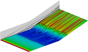Furthermore, the time-averaged flow (averaged from $tu_\infty / L = 60$ to 130) exhibits a spanwise wavelength of $\lambda _z / L \approx 0.33$, as shown in figure 13. Surprisingly, this wavelength agrees well with the most unstable wavelength of mode 4. Note that mode 4 is a stationary mode, and hence it can be better extracted from the time-averaged flow. Note also that the wavelength of the stationary mode 1 is very close to that of the oscillatory modes 2–3. Thus, mode 1 is not distinguished in the time-averaged flow. It is seen in figure 13 that the large-scale spanwise periodicity is confined in the separation bubble. This flow structure is typical of vortical cells moving away from the wall at the centre of a vortex pair (upwash) or towards the wall at the position between two vortex pairs (downwash). In summary, footprints of the global modes revealed by the GSA are well observed in the DNS data.

Figure 13. Time-averaged distribution of the spanwise velocity component at different planes: (a) wall-parallel plane at $y_n/L = 0.009$; (b) $z$–$y$ plane at $x/L = 1.04$; (c) $x$–$y$ plane at $z/L = 0.6$. The density gradient at $z/L = 0$ is shown in panel (a) to highlight the position of the separation bubble.

Figure 14 shows the contours of the real part of the spanwise velocity perturbation $\hat {w}/u_\infty$ for modes 1–4 at their most unstable wavelengths (i.e. $\lambda _z / L = 0.066$, 0.070, 0.079 and 0.349). Note that a sponge layer was implemented from $x/L = 1.9$ to damp the perturbations to zero and allow the use of a simple extrapolation condition at the outflow boundary (Mani Reference Mani2012). For mode 1, most of the perturbations are confined in the downstream half of the separation region, which stretch farther downstream through the reattaching shear layer. It is indicated that these two flow regions are closely coupled with each other. This mode shape is identical to the flow structure captured by the DNS (see figure 6a). A similar eigenfunction was also reported by Sidharth et al. (Reference Sidharth, Dwivedi, Candler and Nichols2017) for a heated ramp flow. By contrast, modes 2–4 are present in the entire separation region. Notably, modes 2 and 3 exhibit streamwise periodicity in the upstream half of the separation bubble, indicating travelling spanwise oblique perturbations associated with temporal oscillations (Sidharth et al. Reference Sidharth, Dwivedi, Candler and Nichols2018).

Figure 14. Real parts of the spanwise velocity perturbation $\hat {w}/u_\infty$ for (a) mode 1 at $\lambda _z / L = 0.066$; (b) mode 2 at $\lambda _z / L = 0.070$; (c) mode 3 at $\lambda _z / L = 0.079$; (d) mode 4 at $\lambda _z / L = 0.349$. The separation and reattachment points are marked with circles.

4.1. Spatio-temporal distribution of the surface heat flux downstream of reattachment

For illustration of the unsteady surface heat flux, an animation showing wall Stanton number snapshots between $tu_\infty /L = 60$ and $tu_\infty /L = 130$ is available in the supplementary movie available at https://doi.org/10.1017/jfm.2020.1093. It is seen that the position, intensity and thickness of the streaks vary irregularly with time, which clearly demonstrates the unsteady behaviour of the surface heat flux. Moreover, some streaks are emerging, while some others disappear. The movement of the streaks seems to have a connection to the movement of the reattachment line. In the following, statistical analyses are performed to characterise the unsteady behaviour of the surface heat flux.

Considering the temporal fluctuation of the surface heat flux downstream of reattachment, its relative standard deviation can be determined as follows:

(4.1)\begin{equation} \widehat{St} = \frac{\sqrt{\displaystyle \frac{1}{N} \sum_{i=1}^{N} (St_i-\overline{St})^{2}}}{\overline{St}}, \end{equation}

where $\overline {St}$ denotes the time-averaged value, and $N$ is the number of sampling points. The relative standard deviation $\widehat {St}$ for all spanwise positions at $x/L = 1.5$ is presented in figure 15. It is clear that $\widehat {St}$ is not constant in the spanwise direction. We note that this spanwise variation is related to the coherent structure shown in figure 13. For example, the strongest fluctuation has a $\widehat {St}$ value of 57 % and is located at $z/L = 0.87$, corresponding to the upwash position in a vortex pair. However, the lowest $\widehat {St}$ is found at $z/L = 0.68$, corresponding to the downwash position between two vortex pairs. This result indicates a direct influence of the separation bubble flow on the downstream heat flux fluctuation, which suggests that the unsteadiness in the reattached flow may be traced back to the separation bubble.

Figure 15. Relative standard deviation of the wall Stanton number for all spanwise positions at $x/L = 1.5$.

To identify a possible transport direction of the flow unsteadiness, a two-point spatio-temporal correlation is employed to evaluate the fluctuation quantities of the wall Stanton number ($St' = St - \overline {St}$),

(4.2)\begin{equation} R_{nm}(\tau)=\frac{\overline{St'_{n}(t)\cdot St'_{m}(t+\tau)}}{\sqrt{\overline{St'^{2}_{n}}} \cdot \sqrt{\overline{St'^{2}_{m}}}}, \end{equation}

where the subscript $n$ denotes the reference point $x/L = 1.5$, $z/L = 0.5$; $m$ corresponds to the position varying in streamwise or spanwise direction; and $\tau$ is the time delay.

Figure 16 shows the calculated correlation maps. It is apparent that a strong correlation exists in the streamwise direction, whereas the correlation in the spanwise direction is quite weak. It means that the primary propagation direction of the unsteadiness is in the streamwise direction. The linear slope of the main structure shown in figure 16(a) by the solid black line indicates the travelling speed of the unsteadiness, which is evaluated approximately by $0.7u_\infty$.

Figure 16. Two-point temporal correlation maps for the wall Stanton number in (a) the streamwise direction and (b) the spanwise direction. Reference point is located at $x/L= 1.5$, $z/L= 0.5$.

In terms of the fluctuation frequency, the PSD of the wall Stanton number signal shown in figure 9 is firstly considered. Note that the calculation is performed for the time period of $tu_\infty /L = 60 \sim 130$ with a sampling frequency of 0.57 MHz. Welch's method (Welch Reference Welch1967) is employed for the spectral estimation with seven segments and 50 % overlap. A Hamming window is used for weighting the data on each segment prior to fast Fourier transform processing. The above setting yields the length of an individual segment being $17.5L/u_\infty$. The resulting PSD is shown in figure 17(a). It is seen that the surface heat flux signal has a broadband low-frequency feature, and the dominant non-dimensional frequencies ($\,f\kern0.5pt L/u_\infty$) are lower than 1 and approximately centred at $\,f\kern0.5pt L/u_\infty = 0.15$.

Figure 17. (a) Power spectral density of the wall Stanton number signal at $x/L = 1.5$ and $z/L = 0.5$. (b) Power spectral density map for all spanwise positions at $x/L = 1.5$.

Figure 17(b) provides the PSD contour for the wall Stanton number by considering all spanwise positions at $x/L = 1.5$. The low-frequency characteristic holds at all spanwise positions, though a spanwise variation of amplitude exists. In general, groups of high amplitude are present at certain spanwise positions. This is consistent with the spanwise variation of the relative standard deviation shown in figure 15. It is noted that the frequencies of modes 2 and 3 found by the previous GSA are 0.224 and 0.579, respectively, which are covered by the broadband spectrum for the wall Stanton number.

4.2. Unsteady flow reattachment

Since the flow reattachment directly influences the downstream reattached flow, it is necessary to study the unsteadiness near reattachment. Figure 18 shows the temporal history of the spanwise-averaged reattachment position and the particular reattachment position on the plane of symmetry ($z/L = 0.5$), in comparison with the downstream wall Stanton number signal. Unlike the pulsation of the reattachment point at $z/L = 0.5$, the spanwise-averaged reattachment point is nearly invariant, indicating a steady state for the spanwise-averaged separation bubble. It should be mentioned that the spanwise-averaged separation position also maintains temporarily invariant. This can be observed in the supplementary animation. Therefore, the well known breathing of the separation bubble in turbulent SWBLI (Priebe & Martín Reference Priebe and Martín2012; Clemens & Narayanaswamy Reference Clemens and Narayanaswamy2014; Pasquariello, Hickel & Adams Reference Pasquariello, Hickel and Adams2017) is absent here. Note however, that the separation bubble size in the present case is much larger than those in the turbulent flow.

Figure 18. Temporal history of reattachment positions in comparison with wall Stanton number. The black solid line corresponds to the reattachment position for the plane of symmetry ($z/L = 0.5$) and the red solid line to the spanwise-averaged reattachment position. The dashed line is the wall Stanton number signal shown in figure 9.

By comparing the temporal distribution of the reattachment position at $z/L = 0.5$ and the downstream wall Stanton number, a generally opposite trend is apparent in figure 18; when the reattachment position moves downstream, the Stanton number decreases, and vice versa. This opposite trend reveals a close link between flow reattachment and the downstream surface heat flux streaks, which can be explained by showing the streamline topology at reattachment. For the flow reattachment with accompanying streamwise streaks, Ginoux (Reference Ginoux1971) and Inger (Reference Inger1977) proposed a three-dimensional topology of the limiting streamline near reattachment, which was further improved by Cao et al. (Reference Cao, Klioutchnikov and Olivier2019a) and Kavun et al. (Reference Kavun, Lipatov and Zapryagaev2019). As shown in figure 19(a), a series of singularities (nodes and saddle points) are distributed along the reattachment line, and nodes are located upstream of saddle points, which is confirmed by the present DNS results (see figures 8 and 19b). In addition, this streamline topology is similar to that induced by global instability (Sidharth et al. Reference Sidharth, Dwivedi, Candler and Nichols2018). This similarity suggests a continuous influence of global instability on the saturated flow. Downstream of a saddle point, the flow is forced to coalesce, resulting in a lift-up effect of the reattached boundary layer. As a result of a three-dimensional reattaching shear layer and this flow topology at reattachment, a hot streak (large $St$) is always located downstream of a node and a cold streak (small $St$) downstream of a saddle point. Therefore, the pulsation of the reattachment position is accompanied by a variation of the downstream surface heat flux. In addition, the spectra of the reattachment position signal are the same as that of the wall Stanton number due to its opposite behaviour.

Figure 19. (a) Streamline topology near reattachment proposed by Cao et al. (Reference Cao, Klioutchnikov and Olivier2019a). (b) Streamlines on a near-wall plane ($y_n/L = 0.0008$) embedded in the wall Stanton number contour at $tu_\infty /L = 100$. Here N and S denote nodes and saddle points, respectively.

The above analyses revealed the unsteady behaviour of the streamwise heat flux streaks and their connection to the flow reattachment. It is shown that the surface heat flux are coupled with the pulsation of reattachment line, oscillating at relatively low frequencies. These results indicate that the unsteadiness originates from the three-dimensional separation bubble. As revealed by the GSA performed earlier, two oscillatory global modes exist in the separation bubble with respect to the two-dimensional base flow. Hence, one may conceive that the unsteadiness in the saturated separation bubble flow is triggered by the global instability. In what follows, the separation bubble flow with respect to its saturated state is examined in an attempt to uncover its instability.