2.1 Vortex-sheet-based flow model

Assume that the rigid-body motion of the airfoil in a quiescent environment can be decomposed into a translational motion of velocity $-U(t)$ and a rotational motion of angular velocity $\unicode[STIX]{x1D6FA}(t)$ . Both the translational and the rotational motions can be incorporated into the boundary condition at the solid–fluid interface. As shown in figure 1, flow separation near the leading edge and at the sharp trailing edge of the airfoil causes the formation of two free vortex sheets in the wake. In a Cartesian coordinate system with the origin fixed at the rotation centre, the complex potential of the flow around an airfoil with angle of attack, $\unicode[STIX]{x1D6FC}(t)$ , can be formulated as

where $z$ is the complex position, $s$ is the curve length between the separation point and a vortex element along a vortex sheet and $\unicode[STIX]{x1D6FE}$ is the vortex-sheet strength (circulation per unit length). The subscripts $_{L}$ and $_{T}$ denote the properties associated with the leading-edge and trailing-edge vortex sheets, respectively. So $S_{L}$ and $S_{T}$ represent the total lengths of the leading-edge and trailing-edge vortex sheets, respectively.

In (2.1), $w_{b}(z,t)$ represents the flow induced by the body motion of the airfoil, and is usually associated with the so-called ‘bound vortex’. Therefore, the ‘bound vortex’ can be viewed as a substitute for the solid body so that the non-penetration boundary condition can still be satisfied at the fluid–solid interface while the solid body is removed from the flow model. Again, we note here that the ‘body term’ or the ‘bound vortex’ implicitly accounts for the effects of translation, rotation or deformation, and more details will be provided in § 2.2. In general, the ‘bound vortex’ can be realized by placing image vortices inside the solid body for a Joukowski airfoil or a flat plate, where the strength and location of the image vortices can be first decided from Milne-Thomson’s circle theorem (Milne-Thomson Reference Milne-Thomson1958) in the circle plane and then mapped back to the physical plane. However, for an arbitrarily shaped airfoil which cannot be easily mapped to a circle, an analytical solution for $w_{b}(z,t)$ is not available. In this case, the ‘bound vortex’ can be realized by placing a bound vortex sheet along the surface of the airfoil as shown in figure 1, and $w_{b}(z,t)$ becomes

where the subscript $_{B}$ denotes the properties associated with the bound vortex sheet. Note here that $s$ for the bound vortex sheet starts from the trailing edge with a counter-clockwise direction, and $S_{B}$ is the total length of the bound vortex sheet.

Combining (2.1) and (2.2) and taking the derivative $\text{d}w/\text{d}z$ , we obtain the complex-conjugate velocity field, $\bar{V}(z,t)=u(z,t)-\text{i}v(z,t)$ , in the form

It should be noted that the velocity field represented by (2.3) is singular on the vortex sheets, where the jump of the tangential component of velocity is equal to the strength of the vortex sheet (Saffman Reference Saffman1992). More details regarding the evaluation of the vortex sheets will be discussed in §§2.2 and 3. At this point, the calculation of the entire flow field is reduced to determining the strength and distribution of only a few finite length vortex sheets.

2.2 Bound vortex sheet

The instantaneous velocity field around an airfoil can now be decided if the two free vortex sheets and one bound vortex sheet are given. This requires knowing the strengths and positions of the vortex sheets ( $\unicode[STIX]{x1D6FE}_{L},\unicode[STIX]{x1D6FE}_{T},\unicode[STIX]{x1D6FE}_{B},z_{L},z_{T},z_{B}$ ). Considering the case where the flow initially remains fully attached, this indicates no flow separation or free vortex sheet existed at $t=0$ . Under this assumption, $\unicode[STIX]{x1D6FE}_{L}$ , $\unicode[STIX]{x1D6FE}_{T}$ , $z_{L}$ , $z_{T}$ for later times might be found through solving the formation and evolution of the free vortex sheets. So we assume that $\unicode[STIX]{x1D6FE}_{L}$ , $\unicode[STIX]{x1D6FE}_{T}$ , $z_{L}$ , $z_{T}$ are known in order to solve the bound vortex sheet at any given time. Furthermore, the position of the bound vortex sheet, $z_{B}$ , is also known as it coincides with the surface of the airfoil at any time. As a result, the main task here is to solve for the vortex-sheet strength $\unicode[STIX]{x1D6FE}_{B}$ . We should note that a bound vortex sheet is treated differently from a free vortex sheet since $z_{B}$ is prescribed. Actually, the free vortex sheet is applied to represent the physical free shear layer, while the bound vortex sheet is introduced to ‘mimic’ the effect of a solid boundary. Therefore, it is expected that the primary role of the bound vortex sheet is to satisfy the non-penetration boundary condition, which can be expressed as

where $\boldsymbol{u}(z^{\prime })=(u(z^{\prime }),v(z^{\prime }))$ is the flow velocity at the surface of the airfoil, $z_{B}$ , and $\hat{\boldsymbol{n}}(z^{\prime })$ is the unit normal vector to the surface. Note that the definitions for $z^{\prime }$ and $s^{\prime }$ only apply to the current section. Also, time $t$ is dropped here and in following derivations for simplicity although they should be satisfied instantaneously. $\boldsymbol{u}_{b}(z^{\prime })$ is the velocity associated with the surface element of the airfoil so it generally describes the deformation of an airfoil. However, $\boldsymbol{u}_{b}(z^{\prime })$ can be also applied to account for the translational motion in the complex-conjugate form, $-|U|\text{e}^{-\text{i}\unicode[STIX]{x1D6FC}}$ , and the rotational motion in the complex-conjugate form, $-\text{i}\unicode[STIX]{x1D6FA}\bar{z}^{\prime }$ , where $\bar{z}^{\prime }$ denotes the complex conjugate of $z^{\prime }$ .

Since the bound vortex sheet is placed at the surface of the airfoil, it creates a velocity jump across $z_{B}$ . Based on (2.3) and the definition of a vortex sheet (Saffman Reference Saffman1992), the two limiting values for $u^{\pm }(z^{\prime })-\text{i}v^{\pm }(z^{\prime })=\bar{V}_{B}^{\pm }(z^{\prime })$ can be derived as

where $\unicode[STIX]{x2A0D}$ denotes the Cauchy principal value which excludes the vorticity at $z^{\prime }$ from the integral. $\text{d}z^{\prime }|\text{d}z^{\prime }|^{-1}$ is the complex form of the unit tangential vector, $\hat{\boldsymbol{s}}(z^{\prime })$ , at the surface of the airfoil. With $\hat{\boldsymbol{s}}(z^{\prime })$ pointing in the counter-clockwise direction of the airfoil body, $\bar{V}_{B}^{+}(z^{\prime })$ becomes the velocity limit when the bound vortex sheet is approached from the outside of the airfoil, whereas $\bar{V}_{B}^{-}(z^{\prime })$ is the velocity limit when the vortex sheet is approached from the inside. Since $\boldsymbol{u}(z^{\prime })$ is the flow velocity outside the surface of the airfoil, it should take the value $\bar{V}_{B}^{+}(z^{\prime })$ . With $\hat{\boldsymbol{n}}(z^{\prime })$ written as $-\text{i}\,\text{d}z^{\prime }|\text{d}z^{\prime }|^{-1}$ , equation (2.4) has the complex form

Ideally, equation (2.6) would give the strength of the bound vortex sheet, $\unicode[STIX]{x1D6FE}_{B}$ , if $\unicode[STIX]{x1D6FE}_{L}$ , $\unicode[STIX]{x1D6FE}_{T}$ , $z_{L}$ , $z_{T}$ and $z_{B}$ are given. However, a general analytical solution to (2.6) does not exist for an arbitrarily shaped airfoil. Fortunately, it is possible to solve this problem numerically by discretizing the bound vortex sheet into piecewise linear vortex panels, the details of which will be discussed in § 6.1.

It should be noted that the strength of the bound vortex sheet $\unicode[STIX]{x1D6FE}_{B}$ can be expressed as $\unicode[STIX]{x1D6FE}_{B}=\boldsymbol{u}_{f}\boldsymbol{\cdot }\hat{\boldsymbol{s}}$ , where $\boldsymbol{u}_{f}$ represents the potential flow velocity at the fluid–solid boundary. With a no-slip boundary condition, $\unicode[STIX]{x1D6FE}_{B}$ can be divided into two terms, $\unicode[STIX]{x1D6FE}_{b}$ and $\unicode[STIX]{x1D6FE}_{\unicode[STIX]{x1D6FE}}$ , according to Eldredge (Reference Eldredge2010). $\unicode[STIX]{x1D6FE}_{b}$ is purely associated with the body-surface motion relative to the reference frame, and it can be estimated from $\unicode[STIX]{x1D6FE}_{b}=\boldsymbol{u}_{b}\boldsymbol{\cdot }\hat{\boldsymbol{s}}$ . $\unicode[STIX]{x1D6FE}_{\unicode[STIX]{x1D6FE}}$ is the physical vortex sheet corresponding to the viscous shear layer, which is given by $\unicode[STIX]{x1D6FE}_{\unicode[STIX]{x1D6FE}}=\unicode[STIX]{x1D6FE}_{B}-\unicode[STIX]{x1D6FE}_{b}$ . Therefore, $\unicode[STIX]{x1D6FE}_{\unicode[STIX]{x1D6FE}}$ is invariant regardless of the reference frame being global or body fixed, while both $\unicode[STIX]{x1D6FE}_{b}$ and $\unicode[STIX]{x1D6FE}_{B}$ could change as the reference frame changes. To avoid ambiguity, $\unicode[STIX]{x1D6FE}_{B}$ in this study only represents the bound vortex sheet in the global reference frame.

2.3 Force and torque

Following previous studies (Wu Reference Wu1981; Eldredge Reference Eldredge2010), the aerodynamic force applied on the airfoil can be estimated based on the rate of change of the total impulse in the form

where $\boldsymbol{x}$ is the position vector of a vortex-sheet element. $\unicode[STIX]{x1D738}=\unicode[STIX]{x1D6FE}\hat{\boldsymbol{k}}$ , where $\hat{\boldsymbol{k}}$ is the unit vector normal to the 2-D plane and $\unicode[STIX]{x1D6FE}$ in this work should be substituted with $\unicode[STIX]{x1D6FE}_{L}$ , $\unicode[STIX]{x1D6FE}_{T}$ and $\unicode[STIX]{x1D6FE}_{B}$ for $S_{L}$ , $S_{T}$ and $S_{B}$ , respectively. $\unicode[STIX]{x1D70C}$ is the density. $\sum S$ represents the entire vortex-sheet system, $\sum S=S_{L}+S_{T}+S_{B}$ . Similarly, the total torque exerted by the fluid on the airfoil can be obtained from

The main advantage of (2.7) and (2.8) is that the calculations of force and torque are completely transformed into the dynamics of the bound and wake vortices, which can be explicitly obtained from this aerodynamic model. Equations (2.7) and (2.8) will be used to estimate aerodynamic force and torque for all simulations in § 6.

3.1 Previous studies and main challenge

We first consider a simple case, where the vortex sheet is formed at the edge of a flat plate or a cusped trailing edge of an airfoil. Without considering the viscous effect, a typical way of deciding the vortex-sheet formation at the trailing edge is the classical steady Kutta condition. This condition requires the flow velocity at the trailing edge to be finite or the loading at the trailing edge to be zero, based on the physical sense that flow cannot turn around a sharp edge. The application of this condition for a flat plate or a Joukowski airfoil (with cusped trailing edge) has already been demonstrated in several previous works (Streitlien & Triantafyllou Reference Streitlien and Triantafyllou1995; Yu et al. Reference Yu, Tong and Ma2003; Ansari et al. Reference Ansari, Zbikowski and Knowles2006a ; Xia & Mohseni Reference Xia and Mohseni2013a ) among others. Basically, this condition is equivalent to enforcing a stagnation point at the trailing edge in the transformed circle plane. However, Xia & Mohseni (Reference Xia and Mohseni2014) recently pointed out that a stagnation point generally does not exist at the trailing edge for the case of body rotation. As a result, they proposed to implement the unsteady Kutta condition by relaxing the trailing-edge point of the circle plane from totally stagnant to only stagnant in the tangential direction of the surface, which still conforms to the classical Kutta condition in the sense of preventing flow around the sharp edge. Here, we emphasize that these steady and unsteady Kutta conditions are problem dependent, meaning they only apply to a flat plate or an airfoil that can be mathematically mapped to a circle.

Alternatively, Jones (Reference Jones2003) modelled the flow around a flat plate using a bound vortex sheet coincident with the plate and two free vortex sheets that are emanating from the plate’s two sharp edges, which is similar to the flow model presented here for an airfoil. By removing the singularities of the flow velocity at the trailing edge, which complies with the classical Kutta condition that flow velocity should be finite at a sharp edge, Jones managed to derive an analytical unsteady Kutta condition. This condition can be summarized as follows:

1. (i) $\unicode[STIX]{x1D6FE}_{g}=\unicode[STIX]{x1D6FE}_{E}$ ;

2. (ii) $u_{g}=u_{E}$ ;

3. (iii) $\unicode[STIX]{x1D703}_{g}=0$ .

Here, $\unicode[STIX]{x1D6FE}_{g}$ , $u_{g}$ and $\unicode[STIX]{x1D703}_{g}$ represent the strength, tangential velocity (relative to the edge), and angle (relative to the tangent of the plate) of the forming vortex sheet, respectively. $\unicode[STIX]{x1D6FE}_{E}$ is the strength of the bound vortex sheet at the sharp edge, and $u_{E}$ is the average tangential slip between the bound vortex sheet and the plate at the edge. Therefore, Jones’ unsteady Kutta condition allows the analytical calculation of the strength, velocity and direction of the forming vortex sheet for the sharp edge of a flat plate or a cusped airfoil, based on the existing bound vortex sheet. However, the current work is concerned with a general-shaped airfoil, for which Jones’ unsteady Kutta condition might not be suitable. Specifically, if there is a finite angle, $\unicode[STIX]{x0394}\unicode[STIX]{x1D703}_{0}\in [0,\unicode[STIX]{x03C0})$ , between the upper and lower surfaces of the trailing edge, $\unicode[STIX]{x1D703}_{g}$ , of the forming vortex sheet would be ambiguous.

This challenge is further explained below. Since the forming vortex sheet moves with the fluid as a material sheet, it resembles a streakline released from the trailing edge in the body-fixed reference frame. Recognizing that at the origin of a streakline the directions of the streakline and the streamline are identical to each other, this indicates that the ambiguity of the vortex-sheet direction is equivalent to the ambiguity of the stagnation streamline direction. In fact, for steady trailing-edge flow where the shedding of vorticity vanishes ( $\unicode[STIX]{x1D6FE}_{g}=0$ ), Poling & Telionis (Reference Poling and Telionis1986) pointed out that the steady Kutta condition requires the stagnation streamline to bisect the wedge angle of a finite-angle trailing edge. Otherwise, an unbalance between the upper and lower shear layers near the trailing edge would cause a non-zero vorticity generation which would be naturally unsteady. According to this argument, an unsteady trailing-edge flow naturally generates vorticity and causes the stagnation streamline to divert from the wedge bisector line, which has been confirmed experimentally (Ho & Chen Reference Ho and Chen1981; Poling & Telionis Reference Poling and Telionis1986). A prominent theory for the unsteady situation has been proposed by Giesing (Reference Giesing1969) and Maskell (Reference Maskell1971) that the stagnation streamline is an extension of one of the two tangents at the trailing edge. Although Basu & Hancock (Reference Basu and Hancock1978) has provided extensive discussion supporting the Giesing–Maskell model, a notable drawback of this model is that it does not reduce to the steady-state solution in the limit of vanishing vorticity. Furthermore, Poling & Telionis (Reference Poling and Telionis1986) reported that the Giesing–Maskell model holds approximately for large rate of vorticity generation, whereas the stagnation streamline direction changes smoothly between the two tangents of the trailing edge when vorticity generation is low.

3.2 The condition for a finite-angle trailing edge

In this study, we seek to derive an unsteady Kutta condition for a finite-angle trailing edge to analytically determine $\unicode[STIX]{x1D6FE}_{g}$ , $u_{g}$ , and $\unicode[STIX]{x1D703}_{g}$ associated with the forming vortex sheet. According to our previous study of an unsteady flat plate (Xia & Mohseni Reference Xia and Mohseni2013a , Reference Xia and Mohseni2014), the unsteady Kutta condition can be implemented numerically by satisfying the condition

where $\boldsymbol{u}_{g}$ is the vector form of the vortex-sheet velocity relative to the trailing edge and $\hat{\boldsymbol{n}}_{g}$ is the unit vector normal to the vortex sheet at the trailing edge as shown in figure 2. Basically, equation (3.1) enforces the streamline to be tangential to the forming vortex sheet.

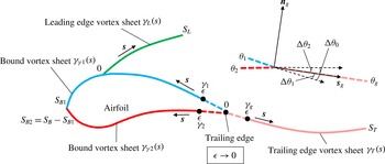
Figure 2. The vortex-sheet configuration for (3.2).

Here, we shall extend (3.1) to the situation of a finite-angle trailing edge to express $\boldsymbol{u}_{g}$ in terms of $\unicode[STIX]{x1D6FE}_{g}$ and $\unicode[STIX]{x1D703}_{g}$ , as well as other parameters associated with the instantaneous background flow and the bound vortex sheet. We assume the flow field changes smoothly so that all vortex sheets are smooth curves near the trailing edge and their strengths also vary smoothly along the sheets. The vortex-sheet system for this calculation is illustrated in figure 2, where $\unicode[STIX]{x1D6FE}_{1}$ and $\unicode[STIX]{x1D6FE}_{2}$ are the bound vortex strengths and $\unicode[STIX]{x1D6FE}_{g}$ is the strength of the forming vortex sheet as it approaches the trailing edge. Noting that the vortex-sheet strength is not well defined at the trailing-edge point, where $\unicode[STIX]{x1D6FE}_{1}$ , $\unicode[STIX]{x1D6FE}_{2}$ and $\unicode[STIX]{x1D6FE}_{g}$ are discontinuous with each other, the trailing-edge point is actually a singularity point in the vortex-sheet system. Fortunately, according to the Birkhoff–Rott equation (Lin Reference Lin1941; Rott Reference Rott1956; Birkhoff Reference Birkhoff1962), $\boldsymbol{u}_{g}$ should be estimated in the desingularized flow field excluding the vorticity at the trailing edge point. This allows us to represent $\boldsymbol{u}_{g}$ , based on the vortex-sheet configuration of figure 2 and (2.3), in the limit form

where $\bar{V}_{CT}$ is the velocity difference associated with the coordinate transformation from the global reference frame to the body-fixed reference frame. $t$ in (2.3) is dropped here for brevity. Recall the discussion of the bound vortex sheet in § 2.2, $\unicode[STIX]{x1D6FE}_{\unicode[STIX]{x1D6FE}}(s)$ rather than $\unicode[STIX]{x1D6FE}_{B}(s)$ should be used here for velocity calculation because $\unicode[STIX]{x1D6FE}_{b}(s)=0$ in the body-fixed reference frame. For convenience, we further divide $\unicode[STIX]{x1D6FE}_{\unicode[STIX]{x1D6FE}}(s)$ into two parts, $\unicode[STIX]{x1D6FE}_{\unicode[STIX]{x1D6FE}1}(s)$ and $\unicode[STIX]{x1D6FE}_{\unicode[STIX]{x1D6FE}2}(s)$ , as shown in figure 2. The relationships between the original and the divided bound vortex sheets are given by $\unicode[STIX]{x1D6FE}_{\unicode[STIX]{x1D6FE}1}(s)=\unicode[STIX]{x1D6FE}_{\unicode[STIX]{x1D6FE}}(s)$ and $z_{B1}(s)=z_{B}(s)$ for $0<s\leqslant S_{B1}$ , and $\unicode[STIX]{x1D6FE}_{\unicode[STIX]{x1D6FE}2}(s)=\unicode[STIX]{x1D6FE}_{\unicode[STIX]{x1D6FE}}(S_{B}-s)$ and $z_{B2}(s)=z_{B}(S_{B}-s)$ for $0<s\leqslant (S_{B}-S_{B1})$ , where $S_{B1}$ and $S_{B2}$ satisfy $S_{B1}+S_{B2}=S_{B}$ . In this way, the two bound vortex sheets both ‘stem’ from the trailing edge, meaning $\lim _{\unicode[STIX]{x1D716}\rightarrow 0}z_{B1}(\unicode[STIX]{x1D716})=\lim _{\unicode[STIX]{x1D716}\rightarrow 0}z_{B2}(\unicode[STIX]{x1D716})$ , and $\lim _{\unicode[STIX]{x1D716}\rightarrow 0}\unicode[STIX]{x1D6FE}_{\unicode[STIX]{x1D6FE}1}(\unicode[STIX]{x1D716})=\unicode[STIX]{x1D6FE}_{1}$ and $\lim _{\unicode[STIX]{x1D716}\rightarrow 0}\unicode[STIX]{x1D6FE}_{\unicode[STIX]{x1D6FE}2}(\unicode[STIX]{x1D716})=\unicode[STIX]{x1D6FE}_{2}$ .

The main challenge of calculating (3.2) is that the integrands of $\int _{\unicode[STIX]{x1D716}}^{S_{T}}$ , $\int _{\unicode[STIX]{x1D716}}^{S_{B1}}$ and $\int _{\unicode[STIX]{x1D716}}^{S_{B2}}$ become singular as $\unicode[STIX]{x1D716}\rightarrow 0$ . As a remedy, we only evaluate its leading-order terms as demonstrated in appendices A and B. Based on the smoothness assumption of the vortex sheets, there exist finite values, $\unicode[STIX]{x1D716}_{1}$ , $\unicode[STIX]{x1D716}_{2}$ and $\unicode[STIX]{x1D716}_{T}$ , so that $\unicode[STIX]{x1D6FE}_{\unicode[STIX]{x1D6FE}1}(s)$ and $z_{B1}(s)$ are smooth on $[0,\unicode[STIX]{x1D716}_{1}]$ , $\unicode[STIX]{x1D6FE}_{\unicode[STIX]{x1D6FE}2}(s)$ and $z_{B2}(s)$ are smooth on $[0,\unicode[STIX]{x1D716}_{2}]$ , and $\unicode[STIX]{x1D6FE}_{T}(s)$ and $z_{T}(s)$ are smooth on $[0,\unicode[STIX]{x1D716}_{2}]$ . Accordingly, equation (3.2) can be divided as

Applying appendix A to the first three integrals and appendix B to the last four integrals yields

where $\bar{V}_{add}$ represents all additional terms of $o(\ln (\unicode[STIX]{x1D716}))$ as $\unicode[STIX]{x1D716}\rightarrow 0$ . $\unicode[STIX]{x1D703}_{1}$ , $\unicode[STIX]{x1D703}_{2}$ and $\unicode[STIX]{x1D703}_{g}$ correspond to the angles of the vortex sheets ( $\unicode[STIX]{x1D6FE}_{\unicode[STIX]{x1D6FE}1}$ , $\unicode[STIX]{x1D6FE}_{\unicode[STIX]{x1D6FE}2}$ and $\unicode[STIX]{x1D6FE}_{T}$ ) in the complex domain as they approach the trailing edge. Now, we combine (3.4) and $\text{Im}\{\bar{V}_{g}\text{e}^{\text{i}\unicode[STIX]{x1D703}_{g}}\}=0$ (the complex form of (3.1)) and then divide both sides by the leading-order term, $\ln (\unicode[STIX]{x1D716})$ , to obtain $\unicode[STIX]{x1D6FE}_{g}+\unicode[STIX]{x1D6FE}_{1}\cos (\unicode[STIX]{x1D703}_{g}-\unicode[STIX]{x1D703}_{1})+\unicode[STIX]{x1D6FE}_{2}\cos (\unicode[STIX]{x1D703}_{g}-\unicode[STIX]{x1D703}_{2})=0$ . Together with the angle relations defined in figure 2, the unsteady Kutta condition takes the form

For the case of a flat plate or a cusped trailing edge, where both $\unicode[STIX]{x0394}\unicode[STIX]{x1D703}_{1}$ and $\unicode[STIX]{x0394}\unicode[STIX]{x1D703}_{2}$ are zero, equation (3.5) is reduced to $\unicode[STIX]{x1D6FE}_{g}=\unicode[STIX]{x1D6FE}_{1}+\unicode[STIX]{x1D6FE}_{2}$ , which is consistent with condition (i) of § 3.1 given by Jones (Reference Jones2003). For a finite-angle trailing edge, equation (3.5) tells us that the strength of the forming vortex sheet $\unicode[STIX]{x1D6FE}_{g}$ depends on its direction $\unicode[STIX]{x1D703}_{g}$ and the strengths of its adjacent bound vortex sheets, $\unicode[STIX]{x1D6FE}_{1}$ and $\unicode[STIX]{x1D6FE}_{2}$ . In § 5, equation (3.5) will be combined with the momentum balance relation and the conservation of circulation to analytically determine $\unicode[STIX]{x1D6FE}_{g}$ , $u_{g}$ and $\unicode[STIX]{x1D703}_{g}$ of the forming vortex sheet.

4.1 A generalized sheet model for viscous shear layer

In order to properly model the dynamics of a viscous shear layer, here we propose a generalized sheet model on top of the original vortex sheet where all relevant quantities or discontinuities associated with the viscous shear layer are superimposed. A schematic of this modelling approach is illustrated in figure 3. As a first step, a sheet of discontinuity in the streamfunction $\unicode[STIX]{x1D713}$ is placed at the location of the original vortex sheet, so that $\unicode[STIX]{x27E6}\unicode[STIX]{x1D713}(s)\unicode[STIX]{x27E7}$ is equal to the volumetric flow rate of the viscous shear layer in the form

where $\unicode[STIX]{x1D6FF}_{s}$ is the thickness of the shear layer and $u^{s}$ is the tangential velocity component. Thus, the mass conservation for the new sheet can be written in the differential form

where ${\dot{m}}_{e}(s)$ is the per-unit-length mass entrainment associated with the shear layer and $\unicode[STIX]{x1D70C}_{s}$ is the per-unit-length density defined as $\unicode[STIX]{x1D70C}_{s}=\unicode[STIX]{x1D70C}\unicode[STIX]{x1D6FF}_{s}$ .

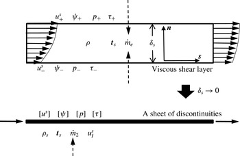
Figure 3. A generalized sheet model to represent a viscous shear layer.

To apply the momentum conservation law to a shear layer, we define a new discontinuity, $\unicode[STIX]{x27E6}\unicode[STIX]{x1D712}\unicode[STIX]{x27E7}$ , in analogy to $\unicode[STIX]{x27E6}\unicode[STIX]{x1D713}\unicode[STIX]{x27E7}$ such that

Therefore, $\unicode[STIX]{x27E6}\unicode[STIX]{x1D712}\unicode[STIX]{x27E7}$ represents the momentum flux associated with the generalized sheet. Furthermore, it is assumed that the new sheet has a characteristic velocity $\boldsymbol{u}_{I}(s)=u_{I}^{s}\hat{\boldsymbol{s}}$ , satisfying $u_{I}^{s}=\unicode[STIX]{x27E6}\unicode[STIX]{x1D712}\unicode[STIX]{x27E7}/\unicode[STIX]{x27E6}\unicode[STIX]{x1D713}\unicode[STIX]{x27E7}$ . In this way, the momentum flux of the shear layer is conserved. To further generalize the vortex sheet, we also superimpose a pressure jump, $\unicode[STIX]{x27E6}p(s)\unicode[STIX]{x27E7}$ , a shear stress jump, $\unicode[STIX]{x27E6}\unicode[STIX]{x1D70F}(s)\unicode[STIX]{x27E7}$ and a surface stress (tension) tensor, $\unicode[STIX]{x1D64F}_{s}$ , which is related to the surface stress $\boldsymbol{t}_{s}$ as $\boldsymbol{t}_{s}=\hat{\boldsymbol{s}}\boldsymbol{\cdot }\unicode[STIX]{x1D64F}_{s}$ in two dimensions. Now, applying the Reynolds transport theorem to a sheet element with a length of $\unicode[STIX]{x0394}s$ , the momentum conservation can be expressed as

where $\boldsymbol{u}_{e}$ is the velocity of the entrained fluid. We note that by assigning proper quantities and discontinuities this new sheet is capable of modelling the dynamics of a viscous shear layer at fluid–fluid or fluid–solid interfaces in single and multiple phase flows.

Next, we apply (4.2) and (4.4) to a special case, the physical vortex sheet $\unicode[STIX]{x1D6FE}_{\unicode[STIX]{x1D6FE}}$ around the surface of an airfoil with free vortex sheets attached. Equation (4.2) can be integrated around the airfoil to give

where the $\sum$ term sums up the mass flux drained into each attached free vortex sheet, and $\unicode[STIX]{x27E6}\unicode[STIX]{x1D713}_{g}\unicode[STIX]{x27E7}$ is the streamfunction jump at the origin of a free vortex sheet. Considering that fluid is physically entrained from the outer flow into the shear layer, the velocity of the entrained fluid should equal the fluid-side velocity of the bound vortex sheet. This gives $\boldsymbol{u}_{e}=\boldsymbol{u}_{f}-\boldsymbol{u}_{b}$ in the body-fixed reference frame, where $\boldsymbol{u}_{b}=u_{b}^{s}\hat{\boldsymbol{s}}+u_{b}^{n}\hat{\boldsymbol{n}}$ . With the non-penetration boundary condition, we have $\boldsymbol{u}_{f}=u_{f}^{s}\hat{\boldsymbol{s}}+u_{b}^{n}\hat{\boldsymbol{n}}$ and $\unicode[STIX]{x1D6FE}_{\unicode[STIX]{x1D6FE}}=u_{f}^{s}-u_{b}^{s}$ . Neglecting surface tension and plugging in (4.2), equation (4.4) can be expanded in the $\hat{\boldsymbol{s}}$ and $\hat{\boldsymbol{n}}$ directions as

Equation (4.7) is still consistent with previous studies (Saffman Reference Saffman1992; Wu, Ma & Zhou Reference Wu, Ma and Zhou2006) in that pressure is continuous across a vortex sheet. This means that the generalized sheet model does not affect the force balance in the normal direction of the sheet. In this sense, equation (2.7) still captures the total force contributed from the pressure term. Now, we further integrate equation (4.6) around the airfoil to obtain

where $\unicode[STIX]{x27E6}\boldsymbol{f}_{\unicode[STIX]{x1D70F}}\unicode[STIX]{x27E7}$ is the jump of the total shear force between the fluid and solid sides of the vortex sheet around the airfoil. Similar to (4.5), the $\sum$ term sums up the momentum flux, $\unicode[STIX]{x27E6}\unicode[STIX]{x1D712}_{g}\unicode[STIX]{x27E7}$ , entering each attached free vortex sheet. $\boldsymbol{u}_{g}^{\ast }$ is the momentum-based characteristic velocity of a free vortex sheet, satisfying $u_{g}^{\ast }=\unicode[STIX]{x27E6}\unicode[STIX]{x1D712}_{g}\unicode[STIX]{x27E7}/\unicode[STIX]{x27E6}\unicode[STIX]{x1D713}_{g}\unicode[STIX]{x27E7}$ . It is noted that the fluid side of $\unicode[STIX]{x1D6FE}_{\unicode[STIX]{x1D6FE}}$ is a free shear surface with zero shear stress, $\unicode[STIX]{x27E6}\boldsymbol{f}_{\unicode[STIX]{x1D70F}}\unicode[STIX]{x27E7}$ is actually the unsteady viscous drag exerted by the solid body, which is not captured by (2.7). Similar to that reported by Liu, Zhu & Wu (Reference Liu, Zhu and Wu2015b ), the term $\unicode[STIX]{x27E6}\unicode[STIX]{x1D713}\unicode[STIX]{x27E7}$ in this study is also the core parameter in drag generation, while here the calculation is performed for the unsteady case. Last, we note that other necessary global quantities and discontinuities can also be superimposed at the location of the original vortex sheet at the solution level for improved force calculation and accurate prediction of vortex-sheet formation, as summarized in table 1.

4.2 Momentum balance for a finite-angle trailing edge

With the generalized sheet model proposed in § 4.1, we are now ready to derive the momentum balance for the merging flow at a finite-angle trailing edge, a schematic of which is provided in figure 4 with the main notations explained in table 2. To formulate the problem, a 2-D material volume $A_{m}$ is defined in the body-fixed reference frame with its boundary $\unicode[STIX]{x2202}A_{m}$ marked by the dashed contour. $\unicode[STIX]{x1D716}_{s}$ is the characteristic length of $A_{m}$ , and is defined as the length of the common interface $S_{\unicode[STIX]{x1D6FE}g}$ between $A_{m1}$ and $A_{m2}$ as shown in figure 4. It is noted that the bulk of the merging area $A_{m}$ is immersed in the inviscid flow outside the sheet system. This is because the inviscid flow also plays an essential part in dictating the flow regime near the trailing edge. In fact, for large Reynolds number situation, where mass and momentum contributions from the viscous shear layer become negligible, the direction of the trailing-edge streamline should be solely governed by the inviscid flow. Here, a few physical assumptions and conditions are listed to simplify this problem.

1. (i) The merging process does not happen until the upper and lower streams meet each other at the trailing edge, so any lead region of $A_{m}$ before the trailing edge should be much smaller than $A_{m}$ itself. To this end, the lengths of $S_{\unicode[STIX]{x1D6FE}1}$ and $S_{\unicode[STIX]{x1D6FE}2}$ are assumed to be $o(\unicode[STIX]{x1D716}_{s})$ , whereas all other surfaces of $A_{m}$ , including $S_{1}$ , $S_{f1}$ , $S_{g-}$ , $S_{g+}$ , $S_{f2}$ and $S_{2}$ , have dimension of $O(\unicode[STIX]{x1D716}_{s})$ .

2. (ii) $S_{f1}$ and $S_{f2}$ coincide with streamlines, so there is no mass flux across the surfaces and $u_{n}=\boldsymbol{u}\boldsymbol{\cdot }\hat{\boldsymbol{n}}_{m}=0$ .

3. (iii) Assuming the flow field changes smoothly, $\unicode[STIX]{x2202}/\unicode[STIX]{x2202}t$ of any quantity is finite.

Figure 4. The formation of a free vortex sheet at a finite-angle trailing edge. The definitions of the main symbols are listed in table 2.

To obtain the momentum balance equations, we start with the mass conservation. Note that the dividing surface $S_{\unicode[STIX]{x1D6FE}g}$ overlaps with the forming vortex sheet, so there is no mass flux across it and the mass conservation for $A_{m}$ can be written separately for $A_{m1}$ and $A_{m2}$ in the form

For the bulk of $A_{m}$ , which contains incompressible isotropic Newtonian fluid, the momentum equation in the body-fixed reference frame is expressed as

where $\unicode[STIX]{x1D749}$ is the shear stress tensor. Here, $\dot{\boldsymbol{u}}_{\unicode[STIX]{x1D6FA}}=-2\unicode[STIX]{x1D734}\times \boldsymbol{u}-\unicode[STIX]{x1D734}\times (\unicode[STIX]{x1D734}\times \boldsymbol{r})-\dot{\boldsymbol{U}}_{b}-\dot{\unicode[STIX]{x1D734}}\times \boldsymbol{r}$ , where $\dot{\boldsymbol{U}}_{b}=-\dot{\boldsymbol{U}}$ represents the linear acceleration of the airfoil and $\boldsymbol{U}$ is the translational background flow velocity at the infinity in the body-fixed reference frame. $\dot{\unicode[STIX]{x1D734}}$ is the angular acceleration of the airfoil and $\boldsymbol{r}$ is the position vector relative to the rotation centre. At this point, the momentum conservation for the whole $A_{m}$ can be derived as

where $S_{\unicode[STIX]{x1D6FE}1}$ , $S_{\unicode[STIX]{x1D6FE}2}$ and $S_{\unicode[STIX]{x1D6FE}g}$ correspond to the vortex sheets in $A_{m}$ and $A_{m-}$ denotes the bulk of $A_{m}$ excluding $S_{\unicode[STIX]{x1D6FE}1}$ , $S_{\unicode[STIX]{x1D6FE}2}$ and $S_{\unicode[STIX]{x1D6FE}g}$ . The first term in the second equation is obtained by integrating equation (4.11), whereas the second term is derived from (4.4) with the pressure jump across a vortex sheet being zero.

Considering the infinitesimal size of the control volume normal to the vortex sheets, any variation of the velocity over $S_{1}$ , $S_{2}$ , $S_{g-}$ and $S_{g+}$ is neglected. Together with condition (ii) of this section, equations (4.9) and (4.10) can be further derived as

where the velocities associated with the vortex sheets ( $u_{1-}$ , $u_{1+}$ , $u_{2-}$ , $u_{2+}$ , $u_{g-}$ and $u_{g+}$ ) are normal to the surfaces of $A_{m}$ and are calculated from $u_{n}=\boldsymbol{u}\boldsymbol{\cdot }\hat{\boldsymbol{n}}_{m}$ . The jump of the streamfunction is applied here to account for the mass flux associated with a vortex sheet, similar to (4.1). And the mass flux associated with the forming vortex sheet is divided into $\unicode[STIX]{x27E6}\unicode[STIX]{x1D713}_{g-}\unicode[STIX]{x27E7}$ and $\unicode[STIX]{x27E6}\unicode[STIX]{x1D713}_{g-}\unicode[STIX]{x27E7}$ by the trailing-edge streamline.

To simplify (4.12), we first apply conditions (i) and (iii) of the current section to argue that the integral associated with $\unicode[STIX]{x2202}(\unicode[STIX]{x1D70C}\boldsymbol{u})/\unicode[STIX]{x2202}t$ has magnitude $O(\unicode[STIX]{x1D716}_{s}^{2})$ . Physically, $p$ is continuous so $\unicode[STIX]{x1D735}p$ should be finite. Moreover, $\unicode[STIX]{x1D735}\boldsymbol{\cdot }\unicode[STIX]{x1D749}=0$ holds for $A_{m-}$ because it corresponds to the inviscid flow outside the vortex sheets. Together with the boundedness of $\dot{\boldsymbol{u}}_{\unicode[STIX]{x1D6FA}}$ , equation (4.12) is reduced to

In the current study, there is no surface tension so $\unicode[STIX]{x1D735}\boldsymbol{\cdot }\unicode[STIX]{x1D64F}_{s}=0$ . $S_{\unicode[STIX]{x1D6FE}g}$ corresponds to the free vortex sheet which physically means $\unicode[STIX]{x27E6}\unicode[STIX]{x1D749}\unicode[STIX]{x27E7}=0$ . Furthermore, $\unicode[STIX]{x27E6}\unicode[STIX]{x1D749}\unicode[STIX]{x27E7}$ is finite on the bound vortex sheets $S_{\unicode[STIX]{x1D6FE}1}$ and $S_{\unicode[STIX]{x1D6FE}2}$ according to (4.6). With condition (i), the right-hand side of (4.15) becomes $o(\unicode[STIX]{x1D716}_{s})$ . Now, applying the velocity boundary conditions of $\unicode[STIX]{x2202}A_{m}$ , the momentum balance can be written in the $\hat{\boldsymbol{s}}_{g}$ and $\hat{\boldsymbol{n}}_{g}$ directions, respectively, in the form

where the superscript $^{\ast }$ denotes the characteristic velocity scale based on the momentum flux of a vortex sheet, similar to (4.8).

In general, the $\unicode[STIX]{x27E6}\unicode[STIX]{x1D713}\unicode[STIX]{x27E7}$ and $u^{\ast }$ terms need to be given or solved for an actual flow. In the current study, for the large Reynolds number situation, the mass and momentum associated with the vortex sheet are neglected as a first approximation. So the $\unicode[STIX]{x27E6}\unicode[STIX]{x1D713}\unicode[STIX]{x27E7}$ and $u^{\ast }$ terms become zero in (4.13), (4.14), (4.16) and (4.17). Furthermore, the terms $O(\unicode[STIX]{x1D716}_{s}^{2})$ and $o(\unicode[STIX]{x1D716}_{s})$ can be neglected in the limit $\unicode[STIX]{x1D716}_{s}\rightarrow 0$ . So (4.17) gives $\unicode[STIX]{x0394}\unicode[STIX]{x1D703}_{1}\boldsymbol{\cdot }\unicode[STIX]{x0394}\unicode[STIX]{x1D703}_{2}\geqslant 0$ . Since

it yields $\unicode[STIX]{x0394}\unicode[STIX]{x1D703}_{1},\unicode[STIX]{x0394}\unicode[STIX]{x1D703}_{2}\geqslant 0$ which means that the direction of the forming vortex sheet should vary between the two tangents of the trailing-edge surfaces. Now, we can combine (4.13), (4.14), (4.16) and (4.17) and cancel $S_{1}$ , $S_{2}$ , $S_{g-}$ and $S_{g+}$ to obtain

This gives the momentum balance at a finite-angle trailing edge for large Reynolds number flow. Equation (4.19) offers another relation between the forming vortex sheet ( $u_{g+}$ , $u_{g-}$ , $\unicode[STIX]{x0394}\unicode[STIX]{x1D703}_{1}$ and $\unicode[STIX]{x0394}\unicode[STIX]{x1D703}_{2}$ ) and the existing bound vortex sheets ( $u_{1+}$ and $u_{2-}$ ). It will be applied in the next section to solve $\unicode[STIX]{x1D6FE}_{g}$ , $u_{g}$ and $\unicode[STIX]{x1D703}_{g}$ of the forming vortex sheet.

6.1 Numerical approach

This section introduces the numerical approaches for implementing the vortex-sheet-based flow model. Mathematically, a vortex sheet can be viewed as a continuous sheet of point singularities of vorticity. Thus, numerical implementation of the model requires discretization of the bound and wake vortex sheets. In this work, the bound vortex sheet and the wake vortex sheet are treated differently based on the following considerations. As the shape of the airfoil is given, each element of the bound vortex sheet is considered to be fixed locally to the surface of the solid body with varying strength to instantaneously satisfy the wall boundary condition. This inspires us to segment the continuous bound vortex sheet into piecewise linear panels, the essence of which is consistent with the traditional panel method (Morino & Kuo Reference Morino and Kuo1974; Katz Reference Katz1981; Katz & Plotkin Reference Katz and Plotkin1991). On the other hand, since the wake vortex sheet is free, the motion of its element follows the Birkhoff–Rott equation while the strength being invariant under inviscid assumption. Thus, the wake vortex sheet would be constantly deforming subject to its background flow. If the same discretization technique as the bound vortex sheet were to be implemented, refinement and reconstruction of the panel system would be necessary to resolve the shrinking or stretching of each sheet element as well as the curvature change. As a result, the numerical cost would grow rapidly as time proceeds, especially when vortex sheet roll up occurs. In the current study, we discretize the wake vortex sheet with an alternative approach, the point-vortex approximation, which is more computationally efficient. The detailed approaches are provided below.

As discussed previously, the key to determining an instantaneous bound vortex sheet is to solve its strength distribution through (2.6). Accordingly, the bound vortex sheet can be discretized into piecewise linear vortex panels as shown in figure 7. For the $n$ th panel, assuming its strength varies linearly from $\unicode[STIX]{x1D6FE}_{B}^{n}$ to $\unicode[STIX]{x1D6FE}_{B}^{n+1}$ , the complex-conjugate velocity at $z$ induced by the vortex-sheet segment corresponding to this panel can be approximated as

where $z_{B}^{n-1}=z_{B}(S_{B}^{n-1})$ and $z_{B}^{n}=z_{B}(S_{B}^{n})$ . For an instantaneous flow, the only unknown parameters are the strengths $\unicode[STIX]{x1D6FE}_{B}^{n}$ and $\unicode[STIX]{x1D6FE}_{B}^{n+1}$ associated with each vortex panel.

Point-vortex approximation is adopted to discretize the wake vortex sheet, similar to numerous previous studies (Moore Reference Moore1974; Krasny Reference Krasny1986a ,Reference Krasny b , Reference Krasny1991; Nitsche & Krasny Reference Nitsche and Krasny1994; Jones Reference Jones2003; Shukla & Eldredge Reference Shukla and Eldredge2007). According to Krasny (Reference Krasny1986a ,Reference Krasny b ), this approximation is ill posed, meaning the discretization errors would grow in time and lead to irregular configuration of the sheet. Krasny proposed to resolve this problem by applying a filtering technique, which replaces the singular term $z^{-1}$ in the complex-conjugate velocity with the so-called vortex-blob kernel, $|z|^{2}[(|z|^{2}+\unicode[STIX]{x1D6FF}_{v}^{2})z]^{-1}$ , where $\unicode[STIX]{x1D6FF}_{v}$ is a small value compared to $|z|$ . As explained by Jones (Reference Jones2003), the essence of this technique is that the desingularization of the velocity kernel would likely to suppress the Kelvin–Helmholtz instability inherent with the discretization at wavelengths below the order of $\unicode[STIX]{x1D6FF}_{v}$ . Figure 7 illustrates how point vortices are distributed to represent the wake vortex sheet. As a result, the complex-conjugate velocity induced by the vortex-sheet segment corresponding to the $n$ th trailing-edge vortex takes the form

where $z_{T}^{n}$ and $\unicode[STIX]{x1D6E4}_{T}^{n}$ are the location and circulation of the $n$ th wake vortex, respectively. We note that $\unicode[STIX]{x1D6E4}_{T}^{n}$ is an invariant and $z_{T}^{n}$ is obtained by evolving the Birkhoff–Rott equation, so they are known quantities for an instantaneous flow.

In accordance with the unsteady Kutta condition developed in § 3.2 and to properly reconcile the different discretization schemes between the bound and wake vortex sheets, a vortex panel of constant strength $\unicode[STIX]{x1D6FE}_{g}$ , namely the $g$ panel, is employed to represent the segment of the wake vortex sheet being formed at the trailing edge. As shown in figure 7, the $g$ panel will be transformed into individual wake vortex as flow evolves, based on the conservation of circulation. The trailing-edge panels are $\unicode[STIX]{x1D716}$ (a small number compared to each panel) distance away from the trailing-edge point, which is consistent with the set-up in (3.2) and figure 2, to account for the discontinuous strength of the vortex-sheet system. The complex-conjugate velocity induced by the vortex-sheet segment corresponding to $g$ panel can be expressed as

where $z_{g}^{0}=z_{T}(\unicode[STIX]{x1D716})$ and $z_{g}^{1}=z_{T}(S_{T}^{1})$ . Now, we have completed the task of discretizing the total vortex-sheet system.

The following summarizes the procedure for advancing the simulation from $t$ to $t^{\prime }=t+\unicode[STIX]{x0394}t$ .

Step 1: Wake evolution. By the end of the previous step, the flow field is solved, so $z_{B}^{n}(t)$ , $\unicode[STIX]{x1D6FE}_{B}^{n}(t)$ , $z_{T}^{n}(t)$ , $\unicode[STIX]{x1D6E4}_{T}^{n}(t)$ , $z_{g}^{1}(t)$ and $\unicode[STIX]{x1D6FE}_{g}(t)$ are known variables. To obtain the wake distribution for the new step, the $g$ panel is first replaced by a new point vortex using

where the latter is essentially the conservation of circulation. Then, $z_{T}^{n}(t^{\prime })$ of each wake vortex is evolved by integrating the Birkhoff–Rott equation with a fourth-order Runge-Kutta scheme.

Step 2: Motion update. Since the motion of the airfoil is prescribed in this study, the translational and rotational motions of the airfoil, $U(t^{\prime })$ and $\unicode[STIX]{x1D6FA}(t^{\prime })$ , need to be updated. If the airfoil is deformable, updating $z_{B}^{n}(t^{\prime })$ is also necessary.

Step 3: $g$ panel addition. The new $g$ panel at $t^{\prime }$ should be added based on the proposed unsteady Kutta condition. This requires a full knowledge of its connecting bound vortex panels at $t^{\prime }$ , which are yet to be computed. Here, the bound vortex panels together with the $g$ panel are solved in a coupled sense. To avoid nonlinearity in solving this coupled system, the direction $\unicode[STIX]{x1D703}_{g}(t^{\prime })$ and shedding velocity $u_{g}(t^{\prime })$ of the $g$ panel are computed from (5.4), (5.1) and (C 10), based on the bound vortex panels of the previous time step. Consequently, $z_{g}^{1}(t^{\prime })$ can be decided from

where $z_{TE}$ is the complex coordinate of the trailing edge point.

Step 4: Equation solving. At this stage, the unknown variables are the strengths of the bound vortex panels and the $g$ panel. In figure 7, $z_{C}^{n}$ marks the control point where the wall boundary condition is satisfied for each panel. Applying the velocity approximations of (6.1), (6.2) and (6.3), the boundary condition specified by (2.5) and (2.6) can be written in the form,

where $D_{nm}$ , $E_{n}$ and $H_{n}$ are coefficients or constants expressed by $z_{C}^{n}$ and other known parameters. For brevity, their detailed expressions are not presented. Furthermore, the Kelvin’s circulation theorem predicts that all vortices in the flow field should satisfy

Therefore, equations (6.7), (6.8) and (3.5) together constitute a $(N_{B}+2)$ th-order linear system, which is solved analytically to give $[\unicode[STIX]{x1D6FE}_{B}^{1}\unicode[STIX]{x1D6FE}_{B}^{2}\ldots \unicode[STIX]{x1D6FE}_{B}^{N_{B}+1}\unicode[STIX]{x1D6FE}_{g}]^{\text{T}}$ . This completes the computation of the entire vortex-sheet system at time $t^{\prime }$ . Last, for flow initialization at $t=0$ , step 4 should be performed with $\unicode[STIX]{x1D6FE}_{g}=0$ and $N^{T}=0$ , so the $(N_{B}+1)$ th-order linear system of the combined equations (6.7) and (6.8) is solved to give the initial strength distribution of the bound vortex sheet.

Figure 8. Non-dimensional bound circulation vs. non-dimensional distance travelled. The Wagner functions for circulation are provided by Ford & Babinsky (Reference Ford and Babinsky2013) and Li & Wu (Reference Li and Wu2015).

6.2 Airfoils in steady background flow

An impulsively started NACA 0012 airfoil is simulated at various angles of attack. In the body-fixed reference frame, the problem is equivalent to that with a background flow abruptly accelerating from zero to a constant. Although the background flow can be treated as a steady flow for $t>0$ , the problem itself is naturally unsteady because of the formation of a starting trailing-edge vortex. Eventually, a steady flow field around the airfoil can be achieved and the lift will saturate as the starting TEV moves downstream. Therefore, the estimation of the circulation shed from the trailing edge is essential to the accurate prediction of lift generation on the airfoil. For an impulsively started thin airfoil or flat plate, Wagner (Reference Wagner1925) has provided the numerical data of the time-variant bound circulation, which can be approximated by $\unicode[STIX]{x1D6E4}_{b}(s^{\ast })/\unicode[STIX]{x1D6E4}_{b}(\infty )\approx 0.9140-0.3151\text{e}^{-s^{\ast }/0.1824}-0.5986\text{e}^{-s^{\ast }/2.0282}$ , given by Ford & Babinsky (Reference Ford and Babinsky2013). $\unicode[STIX]{x1D6E4}_{b}$ is the total bound circulation; $s^{\ast }=s_{t}/c$ where $s_{t}$ is the total distance travelled by the airfoil and $c$ is the chord length. Later, Li & Wu (Reference Li and Wu2015) modified this function as $\unicode[STIX]{x1D6E4}_{b}(s^{\ast })/\unicode[STIX]{x1D6E4}_{b}(\infty )\approx 1-0.8123\text{e}^{-\sqrt{s^{\ast }}/1.276}-0.188\text{e}^{-s^{\ast }/1.211}+3.2683\times 10^{-4}\text{e}^{-s^{\ast 2}/0.892}$ to improve its asymptotic behaviour. In this study, the formation of the TEV is solved by implementing the proposed unsteady Kutta condition at each time step. Then, the total bound circulation can be obtained using Kelvin’s circulation theorem as $\unicode[STIX]{x1D6E4}_{b}=-\unicode[STIX]{x1D6E4}_{TEV}$ , where $\unicode[STIX]{x1D6E4}_{TEV}$ is the total circulation of the trailing-edge vortices. $\unicode[STIX]{x1D6E4}_{TEV}$ can be calculated from $\unicode[STIX]{x1D6E4}_{TEV}=\int \dot{\unicode[STIX]{x1D6E4}}_{g}\,\text{d}t$ , with $\dot{\unicode[STIX]{x1D6E4}}_{g}$ determined by (C 10). Now, we compare the variation of the bound circulation predicted by this model with the approximated Wagner functions in figure 8. A general good agreement can be observed between this result and the modified Wagner function by Li & Wu (Reference Li and Wu2015), except at early stages ( $s^{\ast }<5$ ) where this simulation is slightly different from both Wagner functions. Since Wagner’s simulation was based on a flat plate, this difference is likely to reflect the difference of initial vortex shedding between a finite-camber airfoil and a flat plate. In addition, we note that similar to the Wagner function $\unicode[STIX]{x1D6E4}_{b}(s^{\ast })/\unicode[STIX]{x1D6E4}_{b}(\infty )$ in this simulation is also independent of the angle of attack, although full data are not presented here for brevity.

Figure 9. (a) Lift coefficient ( $C_{l}$ ) vs. non-dimensional distance travelled ( $s^{\ast }$ ) for a NACA 0012 airfoil at various angles of attack. (b) The variation of the angle of the trailing-edge vortex sheet. $\unicode[STIX]{x1D703}_{g}=0$ corresponds to the bisector of the finite-angle trailing edge. $\unicode[STIX]{x1D703}_{g}$ varies between $-\unicode[STIX]{x0394}\unicode[STIX]{x1D703}_{0}/2$ and $\unicode[STIX]{x0394}\unicode[STIX]{x1D703}_{0}/2$ that correspond to the two tangents of the trailing edge.

Figure 9(a) shows the variation of the lift coefficient, $C_{l}$ , for the NACA 0012 airfoil with AoA ranging from $0^{\circ }$ to $10^{\circ }$ . We can verify the saturation trend of the lift coefficient as $s^{\ast }$ increases, which corresponds to the transition of the flow field near the airfoil from unsteady to steady. This transition is also evident in figure 9(b), which shows the variation of the angle ( $\unicode[STIX]{x1D703}_{g}$ ) of the trailing-edge vortex sheet. The trend of $\unicode[STIX]{x1D703}_{g}$ approaching zero also indicates the recovery of condition (iv) of the steady-state Kutta condition summarized by Poling & Telionis (Reference Poling and Telionis1986) (§ 5). Furthermore, it is important to note here that $C_{l}$ at $s^{\ast }=0$ does not start from zero although the bound circulation increases from zero, capturing the added-mass effect. Following recent studies (Xia & Mohseni Reference Xia and Mohseni2013a ; Li & Wu Reference Li and Wu2016) that attributed major lift generation to the effect of vortex motion, this initial lift should be caused by a strong redistribution effect of the vorticity inside the bound vortex sheet.

Figure 10. Lift coefficient ( $C_{l}$ ) vs. angle of attack ( $\unicode[STIX]{x1D6FC}$ ) for (a) a NACA 0012 airfoil and (b) a NACA 2415 airfoil. The experimental data for (a) and (b) are from Sheldahl & Klimas (Reference Sheldahl and Klimas1981) and Abbott, von Doenhoff & Stivers (Reference Abbott, von Doenhoff and Stivers1945), respectively.

The steady-state lift coefficients of this study are compared with experimental data for NACA 0012 and NACA 2415 airfoils, as shown in figure 10. The lift calculations of this model generally match well with experiment at small angles of attack. Furthermore, better agreement can be confirmed for the experimental cases with larger $Re$ . This is because larger $Re$ corresponds to smaller mass and momentum deficits associated with the boundary layer, and is therefore better approximated by the vortex-sheet-based inviscid flow model. Lastly, the lift stall at larger AoA is not captured because this model does not account for flow separation occurring upstream of the trailing edge.

Figure 11. Comparison between flow visualization and simulation for a pitching and heaving NACA 0012 airfoil with $St=0.45$ , $\unicode[STIX]{x1D6FC}_{max}=30^{\circ }$ and $h_{0}=0.75c$ . The flow visualization image is from Schouveiler, Hover & Triantafyllou (Reference Schouveiler, Hover and Triantafyllou2005). The dash line in (b) marks the trajectory of the airfoil.

6.3 Airfoils with unsteady motions

Next, the performance of this vortex-sheet-based aerodynamic model is further justified by simulating a series of unsteady motions of the NACA airfoils. We first investigate a NACA 0012 airfoil with a combined pitching and heaving motion adapted from the experiment of Read, Hover & Triantafyllou (Reference Read, Hover and Triantafyllou2003). For all tests, the chord length and the towing speed are fixed at $c=0.1~\text{m}$ and $U_{tow}=0.4~\text{m}~\text{s}^{-1}$ , respectively. The corresponding Reynolds number is $4\times 10^{4}$ . The pivot for the pitching motion is fixed at $1/3$ chord. The phase difference angle between the pitching and heaving motions is set to $90^{\circ }$ . The characteristic parameters for this motion are the Strouhal number, $St$ , the amplitude of the angle of attack, $\unicode[STIX]{x1D6FC}_{max}$ , and the heave amplitude, $h_{0}$ , which could be adjusted by controlling the pitching and heaving motions. Figure 11 compares the wake structures between this simulation and the flow visualization for a sample case ( $St=0.45$ , $\unicode[STIX]{x1D6FC}_{max}=30^{\circ }$ and $h_{0}=0.75c$ ). The matching of the wake patterns between experiment and simulation is promising. Figure 12 further plots the instantaneous force vectors along the trajectories of two different pitching and heaving motions. The results demonstrate reasonable agreement of the force magnitude and direction between experiment and simulation. This quantitatively validates the performance of the aerodynamic model and the TEV formation conditions for airfoils undergoing unsteady motions. However, since the LEV shedding has not been considered here, the simulations with larger $\unicode[STIX]{x1D6FC}_{max}$ or $St$ values tend to overestimate the force due to possible flow separation after the leading edge.

Figure 12. Comparison of instantaneous thrust vectors between experiment and simulation for a NACA 0012 airfoil. The experimental results are adapted from Read et al. (Reference Read, Hover and Triantafyllou2003). For both cases, $St=0.4$ and $h_{0}=c$ .

Figure 13. The panels on the left show the trajectories and force vectors of different unsteady motions of a NACA 0013 airfoil adapted from the experiment of Izraelevitz & Triantafyllou (Reference Izraelevitz and Triantafyllou2014). The panels on the right show the corresponding simulated wake patterns. Note that this figure only illustrates the unsteady motions of the airfoil, and is not intended for validation.

Figure 14. Result of the symmetric flapping motion corresponding to figure 13(a). (a) Comparison between the measured force coefficients of Izraelevitz & Triantafyllou (Reference Izraelevitz and Triantafyllou2014) and the estimated force coefficients from this simulation. (b) Variations of $\unicode[STIX]{x1D6FC}$ , $U$ and $\unicode[STIX]{x1D703}_{g}$ during one cycle.

Figure 15. Result of the bird-like forward biased downstroke corresponding to figure 13(b). (a) Comparison between measured and estimated force coefficients. (b) Variations of $\unicode[STIX]{x1D6FC}$ , $U$ and $\unicode[STIX]{x1D703}_{g}$ during one cycle.

The unsteadiness of the airfoil motion can be further increased by adding an oscillatory in-line motion on top of the pitching and heaving motion introduced above. Two typical such motions were experimentally studied by Izraelevitz & Triantafyllou (Reference Izraelevitz and Triantafyllou2014), namely, the bird-like forward biased downstroke and the turtle-like backwards moving downstroke. The trajectories of these two motions are shown in figure 13(b) and (c), with the simulated flow field showing the vortical structures in the wake. For comparison, a symmetric flapping case without any additional in-line motion is shown in figure 13(a). The airfoil investigated here is a NACA 0013 type with $c=0.055~\text{m}$ and the pivot at the quarter chord. The Reynolds number is fixed at 11 000 which corresponds to a constant towing speed of $U_{tow}=0.2~\text{m}~\text{s}^{-1}$ . For the pitching and heaving motions of all cases, the characteristic parameters are $St=0.3$ , $\unicode[STIX]{x1D6FC}_{max}=25^{\circ }$ and $h_{0}=c$ . The controlling parameter here is the stroke angle, $\unicode[STIX]{x1D6FD}$ , associated with the added in-line motion. $\unicode[STIX]{x1D6FD}$ is defined based on the $x$ and $y$ positions of the airfoil in the carriage reference frame. The interested readers are referred to Izraelevitz & Triantafyllou (Reference Izraelevitz and Triantafyllou2014) for more details of the original experiment.

For quantitative comparison, the force and torque coefficients are estimated for the unsteady motions presented in figure 13. Similar to Izraelevitz & Triantafyllou (Reference Izraelevitz and Triantafyllou2014), the force coefficients in the $x$ and $y$ directions together with the torque coefficient are defined as $C_{x}=2F_{x}(\unicode[STIX]{x1D70C}U_{tow}^{2}c)^{-1}$ , $C_{y}=2F_{y}(\unicode[STIX]{x1D70C}U_{tow}^{2}c)^{-1}$ and $C_{M}=2T_{\unicode[STIX]{x1D70F}}(\unicode[STIX]{x1D70C}U_{tow}^{2}c^{2})^{-1}$ , respectively, where $F_{x}$ , $F_{y}$ and $T_{\unicode[STIX]{x1D70F}}$ are computed from (2.7) and (2.8). The evolution of $C_{x}$ , $C_{y}$ and $C_{M}$ during each cycle of the prescribed unsteady motions are compared with the experimental data in figures 14(a), 15(a) and 16(a). We again observe a generally good agreement between experiment and simulation, verifying the performance of the proposed flow model. Especially, the results of $C_{y}$ have promising accuracy for all three different cases. Since $C_{y}$ physically represents the lift coefficient, this indicates a prospective application of the current model for lift estimation without modelling the leading-edge separation. However, the void of flow separation in the current simulation seems to have a notable impact on $C_{x}$ , which corresponds to the thrust coefficient. This is reflected by the over-prediction of $C_{x}$ in some cases displayed in figures 14(a) and 15(a). Other than the flow separation, the viscous effect at the solid–fluid interface could also affect the accuracy of predicting thrust or drag using an inviscid flow model.

Figure 16. Result of the turtle-like backwards moving downstroke corresponding to figure 13(c). (a) Comparison between measured and estimated force coefficients. (b) Variations of $\unicode[STIX]{x1D6FC}$ , $U$ and $\unicode[STIX]{x1D703}_{g}$ during one cycle.

To explain the effect of the additional in-line motion on force generation of the airfoil, the variations of the airfoil velocity $U$ and the angle of attack $\unicode[STIX]{x1D6FC}$ are plotted in figures 14(b), 15(b) and 16(b). We can observe that the variations of $\unicode[STIX]{x1D6FC}$ in figures 15 and 16 are identical, and $\unicode[STIX]{x1D6FC}$ only changes in the first half-cycle while it remains zero in the second half-cycle. Since the shedding of strong vorticity mainly occurs at non-zero angles of attack, the force generation associated with vortex shedding should mostly happen during the first half-cycle. In this sense, the first half-cycle is the actual ‘stroke’ while the second half can be considered as the ‘recovery’. However, the different in-line motions during the first half-cycle cause $U$ to increase significantly for the bird-like downstroke in figure 15 and decrease significantly for the turtle-like downstroke in figure 16. This creates stronger and faster trailing-edge vortices of the bird-like downstroke compared to the turtle-like downstroke. As a result, the bird-like downstroke provides much higher lift than the turtle-like downstroke. Finally, we note that the angle of the trailing-edge vortex sheet, $\unicode[STIX]{x1D703}_{g}$ , varies smoothly within the limits of the two tangential directions of the trailing edge, $-\unicode[STIX]{x0394}\unicode[STIX]{x1D703}_{0}/2$ and $\unicode[STIX]{x0394}\unicode[STIX]{x1D703}_{0}/2$ . This also implies the correct implementation of the proposed models, and is in accordance with the experimental observation of Poling & Telionis (Reference Poling and Telionis1986) that the direction of the trailing-edge streamline changes smoothly.