1 Introduction
The aerodynamics of ground vehicles has become a major issue in view of lowering fuel consumption and pollutant emissions. In particular, as one third of the total drag is admitted to be generated at the car’s rear after-body (Hucho Reference Hucho1998), a deeper understanding of the turbulent wake dynamics is thus of prime interest. In view of the large commercial success of minivans and sport utility vehicles, vehicle shapes with vertical after-bodies are nowadays very common.
From the academic point of view, fundamental research investigates simplified geometries such as the Ahmed body (Ahmed, Ramm & Faitin Reference Ahmed, Ramm and Faitin1984). The square-back Ahmed body is a three-dimensional bluff body with a rectangular blunt after-body producing a wide flow separation. It is known to experience a steady supercritical bifurcation in the laminar regime for a Reynolds number of
 $Re\simeq 340$
resulting in a permanent asymmetric state of the wake. This bifurcation was first identified experimentally by Grandemange, Gohlke & Cadot (Reference Grandemange, Gohlke and Cadot2012) and recently confirmed by computation (Evstafyeva, Morgans & Dalla-Longa Reference Evstafyeva, Morgans and Dalla-Longa2017). As the Reynolds number increases, the wake undergoes random switching between two mirror asymmetric states that statistically restores symmetries. These states have been observed up to Reynolds number of
$Re\simeq 340$
resulting in a permanent asymmetric state of the wake. This bifurcation was first identified experimentally by Grandemange, Gohlke & Cadot (Reference Grandemange, Gohlke and Cadot2012) and recently confirmed by computation (Evstafyeva, Morgans & Dalla-Longa Reference Evstafyeva, Morgans and Dalla-Longa2017). As the Reynolds number increases, the wake undergoes random switching between two mirror asymmetric states that statistically restores symmetries. These states have been observed up to Reynolds number of
 $2.5\times 10^{6}$
in the seminal work of Grandemange, Gohlke & Cadot (Reference Grandemange, Gohlke and Cadot2013b
), even with rotating wheels and road effects.
$2.5\times 10^{6}$
in the seminal work of Grandemange, Gohlke & Cadot (Reference Grandemange, Gohlke and Cadot2013b
), even with rotating wheels and road effects.
Since then, many works have reported these asymmetric states (so-called static symmetry-breaking modes) in a variety of geometries with vertical rectangular bases: flat plates (Cadot Reference Cadot2016), square-back Windsor model (Perry et al.
Reference Perry, Almond, Passmore and Littlewood2016a
; Perry, Pavia & Passmore Reference Perry, Pavia and Passmore2016b
; Pavia & Passmore Reference Pavia, Passmore and Wiedemann2018; Pavia, Passmore & Sardu Reference Pavia, Passmore and Sardu2018), square-back Ahmed body both experimentally (Volpe, Devinant & Kourta Reference Volpe, Devinant and Kourta2015; Brackston et al.
Reference Brackston, García De La Cruz, Wynn, Rigas and Morrison2016; Evrard et al.
Reference Evrard, Cadot, Herbert, Ricot, Vigneron and Délery2016; Li et al.
Reference Li, Barros, Borée, Cadot, Noack and Cordier2016; Barros et al.
Reference Barros, Borée, Cadot, Spohn and Noack2017) and numerically (Pasquetti & Peres Reference Pasquetti and Peres2015; Evstafyeva et al.
Reference Evstafyeva, Morgans and Dalla-Longa2017; Lucas et al.
Reference Lucas, Cadot, Herbert, Parpais and Délery2017). Grandemange, Gohlke & Cadot (Reference Grandemange, Gohlke and Cadot2013a
) showed the importance of the rectangular base aspect ratio that can select either left/right or top/bottom asymmetric states of the wake, respectively called
 $y$
- and
$y$
- and
 $z$
-instabilities, where
$z$
-instabilities, where
 $y$
and
$y$
and
 $z$
refer to the wake asymmetry directions as depicted in figure 1. Although the
$z$
refer to the wake asymmetry directions as depicted in figure 1. Although the
 $y$
-instability corresponds to a pure reflectional symmetry breaking, the
$y$
-instability corresponds to a pure reflectional symmetry breaking, the
 $z$
-instability does not, strictly speaking, because of the ground and the body supports (Grandemange et al.
Reference Grandemange, Gohlke and Cadot2013a
).
$z$
-instability does not, strictly speaking, because of the ground and the body supports (Grandemange et al.
Reference Grandemange, Gohlke and Cadot2013a
).
The presence of a permanent asymmetric wake state is also a general property of turbulent wakes of axisymmetric bodies (Grandemange et al.
Reference Grandemange, Gohlke and Cadot2013a
; Rigas et al.
Reference Rigas, Oxlade, Morgans and Morrison2014, Reference Rigas, Morgans, Brackston and Morrison2015; Grandemange, Gohlke & Cadot Reference Grandemange, Gohlke and Cadot2014a
; Gentile et al.
Reference Gentile, Schrijer, Van Oudheusden and Scarano2016, Reference Gentile, Van Oudheusden, Schrijer and Scarano2017), reminiscent of a steady symmetry-breaking bifurcation in the laminar regime leading to an asymmetric state with planar symmetry (Pier Reference Pier2008). In the turbulent regime, the azimuthal phase of the symmetry plane evolves like a random walk (Rigas et al.
Reference Rigas, Morgans, Brackston and Morrison2015) thus exploring all azimuthal angles uniformly. This infinity of directions may be interpreted as a multistable wake in opposition to rectangular bodies that just have two directions, either
 $y$
or
$y$
or
 $z$
. Therefore, three-dimensional bodies with reflectional symmetries or with symmetry of revolution present similar stability properties.
$z$
. Therefore, three-dimensional bodies with reflectional symmetries or with symmetry of revolution present similar stability properties.
Sensitivity analyses of the asymmetric mode to small symmetrical imperfections have been experimentally addressed, either by introducing a steady disturbance in the vicinity of the body (Vilaplana et al. Reference Vilaplana, Grandemange, Gohlke and Cadot2013; Grandemange et al. Reference Grandemange, Gohlke and Cadot2013a , Reference Grandemange, Gohlke and Cadot2014a ; Grandemange, Gohlke & Cadot Reference Grandemange, Gohlke and Cadot2014b ; Brackston et al. Reference Brackston, García De La Cruz, Wynn, Rigas and Morrison2016; Barros et al. Reference Barros, Borée, Cadot, Spohn and Noack2017) or by the main body inclination (Volpe et al. Reference Volpe, Devinant and Kourta2015; Perry et al. Reference Perry, Pavia and Passmore2016b ; Gentile et al. Reference Gentile, Van Oudheusden, Schrijer and Scarano2017). A large majority of these studies show that the imperfection selects the wake on a preferential asymmetric state, thus reducing considerably the multistable dynamics obtained without the imperfections. In the works of Barros et al. (Reference Barros, Borée, Cadot, Spohn and Noack2017), Gentile et al. (Reference Gentile, Van Oudheusden, Schrijer and Scarano2017), this selection is modelled as a pitchfork bifurcation, with either the disturbance size or the misalignment angle as the bifurcation parameter.
Figure 1. Sketches of the recirculating bubbles for the
 $y$
-instability (a) and
$y$
-instability (a) and
 $z$
-instability (b) interpreted from mean wake measurements of Grandemange et al. (Reference Grandemange, Gohlke and Cadot2013a
). Thick arrows display the corresponding base pressure gradients.
$z$
-instability (b) interpreted from mean wake measurements of Grandemange et al. (Reference Grandemange, Gohlke and Cadot2013a
). Thick arrows display the corresponding base pressure gradients.
These asymmetry-related instabilities have a substantial impact on the aerodynamic loading of the body as demonstrated by the fluid–structure interaction experiment of Cadot (Reference Cadot2016). For the Ahmed body, the strategy of symmetrization of the wake either by means of passive (Grandemange et al.
Reference Grandemange, Gohlke and Cadot2014b
; Cadot, Evrard & Pastur Reference Cadot, Evrard and Pastur2015; Evrard et al.
Reference Evrard, Cadot, Herbert, Ricot, Vigneron and Délery2016; Lucas et al.
Reference Lucas, Cadot, Herbert, Parpais and Délery2017) or active (Brackston et al.
Reference Brackston, García De La Cruz, Wynn, Rigas and Morrison2016; Li et al.
Reference Li, Barros, Borée, Cadot, Noack and Cordier2016; Evstafyeva et al.
Reference Evstafyeva, Morgans and Dalla-Longa2017) flow control techniques leads to drag reductions up to
 $9\,\%$
, although it is not clear yet what the real part due the instability suppression alone is.
$9\,\%$
, although it is not clear yet what the real part due the instability suppression alone is.
For sake of simplicity, the wake subjected to the
 $y$
- or
$y$
- or
 $z$
-instability will be called the unstable wake for the remainder of the paper. Variable orientations are often encountered in ground vehicle aerodynamics due to cross-winds introducing yaw, and payload mass modifying ground clearance and pitch. Most of the work done so far considered a body subjected to the
$z$
-instability will be called the unstable wake for the remainder of the paper. Variable orientations are often encountered in ground vehicle aerodynamics due to cross-winds introducing yaw, and payload mass modifying ground clearance and pitch. Most of the work done so far considered a body subjected to the
 $y$
-instability aligned with the incoming flow; only few reported measurements with yaw variations (Cadot et al.
Reference Cadot, Evrard and Pastur2015; Volpe et al.
Reference Volpe, Devinant and Kourta2015; Brackston et al.
Reference Brackston, García De La Cruz, Wynn, Rigas and Morrison2016; Perry et al.
Reference Perry, Pavia and Passmore2016b
) or ground clearance variations (Grandemange et al.
Reference Grandemange, Gohlke and Cadot2013a
; Cadot et al.
Reference Cadot, Evrard and Pastur2015) but none with pitch variations. To the authors’ knowledge, there are no results reported in the literature about the effects of yaw or pitch for a body subjected to the
$y$
-instability aligned with the incoming flow; only few reported measurements with yaw variations (Cadot et al.
Reference Cadot, Evrard and Pastur2015; Volpe et al.
Reference Volpe, Devinant and Kourta2015; Brackston et al.
Reference Brackston, García De La Cruz, Wynn, Rigas and Morrison2016; Perry et al.
Reference Perry, Pavia and Passmore2016b
) or ground clearance variations (Grandemange et al.
Reference Grandemange, Gohlke and Cadot2013a
; Cadot et al.
Reference Cadot, Evrard and Pastur2015) but none with pitch variations. To the authors’ knowledge, there are no results reported in the literature about the effects of yaw or pitch for a body subjected to the
 $z$
-instability. There is then a fundamental issue about the unstable wake response to the body orientation. One may ask the following questions: how does the unstable wake dynamics react to small misalignment? And, what are the consequences on the aerodynamics loading of the body?
$z$
-instability. There is then a fundamental issue about the unstable wake response to the body orientation. One may ask the following questions: how does the unstable wake dynamics react to small misalignment? And, what are the consequences on the aerodynamics loading of the body?
Our experimental strategy is to perform sensitivity analyses changing independently three parameters: the ground clearance
 $c$
, the yaw
$c$
, the yaw
 $\unicode[STIX]{x1D6FD}$
and the pitch
$\unicode[STIX]{x1D6FD}$
and the pitch
 $\unicode[STIX]{x1D6FC}$
with and without the instability by repeating the analyses with a deep rear cavity known as an efficient way to suppress the asymmetric states of the wake (Evrard et al.
Reference Evrard, Cadot, Herbert, Ricot, Vigneron and Délery2016; Lucas et al.
Reference Lucas, Cadot, Herbert, Parpais and Délery2017). The study is extended for a second after-body designed to develop the
$\unicode[STIX]{x1D6FC}$
with and without the instability by repeating the analyses with a deep rear cavity known as an efficient way to suppress the asymmetric states of the wake (Evrard et al.
Reference Evrard, Cadot, Herbert, Ricot, Vigneron and Délery2016; Lucas et al.
Reference Lucas, Cadot, Herbert, Parpais and Délery2017). The study is extended for a second after-body designed to develop the
 $z$
-instability. As introduced by Grandemange et al. (Reference Grandemange, Gohlke and Cadot2013b
), we use the spatial distribution of the pressure at the body base as a topological indicator of the turbulent wake state. Rigas et al. (Reference Rigas, Oxlade, Morgans and Morrison2014, Reference Rigas, Morgans, Brackston and Morrison2015) successfully applied the same technique to an axisymmetric body with a blunt trailing edge and proposed an insightful low-dimensional physical model of the axisymmetric turbulent wake dynamics.
$z$
-instability. As introduced by Grandemange et al. (Reference Grandemange, Gohlke and Cadot2013b
), we use the spatial distribution of the pressure at the body base as a topological indicator of the turbulent wake state. Rigas et al. (Reference Rigas, Oxlade, Morgans and Morrison2014, Reference Rigas, Morgans, Brackston and Morrison2015) successfully applied the same technique to an axisymmetric body with a blunt trailing edge and proposed an insightful low-dimensional physical model of the axisymmetric turbulent wake dynamics.
The paper is organized as follows. The experimental set-up is described in § 2. Results in § 3 are split into two parts, §§ 3.1 and 3.2 respectively investigating the
 $y$
-instability and
$y$
-instability and
 $z$
-instability. For the
$z$
-instability. For the
 $y$
-instability, sensitivity analyses of the base pressure gradient varying ground clearance, yaw and pitch are presented in § 3.1.1 and then repeated in § 3.1.2 with an additional rear deep cavity to suppress the instability. In the third part § 3.1.3, the lateral aerodynamic force is examined in the light of the base pressure gradient contribution with and without the instability. A relationship summarizing the measurements linking lateral force coefficients and the base pressure gradient is given. For the
$y$
-instability, sensitivity analyses of the base pressure gradient varying ground clearance, yaw and pitch are presented in § 3.1.1 and then repeated in § 3.1.2 with an additional rear deep cavity to suppress the instability. In the third part § 3.1.3, the lateral aerodynamic force is examined in the light of the base pressure gradient contribution with and without the instability. A relationship summarizing the measurements linking lateral force coefficients and the base pressure gradient is given. For the
 $z$
-instability, sensitivity analyses of the base pressure gradient varying clearance, yaw and pitch are presented in § 3.2.1 and then yaw sensitivities are repeated in § 3.2.2 for different ground clearances to evidence the two branches of most probable states of the wake. In the third part § 3.2.3, the vertical aerodynamic force is examined in the light of the base pressure gradient contribution. Results lead to two discussions, the role of the phase dynamics for a three-dimensional turbulent wake in § 4.1 and the wake instability adaptation mechanism with the body orientation in § 4.2. Finally, § 5 concludes and offers perspectives on the paper.
$z$
-instability, sensitivity analyses of the base pressure gradient varying clearance, yaw and pitch are presented in § 3.2.1 and then yaw sensitivities are repeated in § 3.2.2 for different ground clearances to evidence the two branches of most probable states of the wake. In the third part § 3.2.3, the vertical aerodynamic force is examined in the light of the base pressure gradient contribution. Results lead to two discussions, the role of the phase dynamics for a three-dimensional turbulent wake in § 4.1 and the wake instability adaptation mechanism with the body orientation in § 4.2. Finally, § 5 concludes and offers perspectives on the paper.
2 Experimental set-up
2.1 Apparatus
The three-dimensional bluff bodies considered in this work are two flat-backed Ahmed bodies (Ahmed et al.
Reference Ahmed, Ramm and Faitin1984) drawn in figure 2. They are composed of the same main body supported by four vertical cylinders and with two interchangeable after-bodies. The characteristic dimensions are given in table 1. The aspect ratio of the rectangular base is
 $W/H=1.174$
for the square-back after-body (model used in Evrard et al. (Reference Evrard, Cadot, Herbert, Ricot, Vigneron and Délery2016)) and
$W/H=1.174$
for the square-back after-body (model used in Evrard et al. (Reference Evrard, Cadot, Herbert, Ricot, Vigneron and Délery2016)) and
 $w_{b}/H=0.940$
for the boat-tailed after-body. The first geometry is known to be subjected to the
$w_{b}/H=0.940$
for the boat-tailed after-body. The first geometry is known to be subjected to the
 $y$
-instability (Evrard et al.
Reference Evrard, Cadot, Herbert, Ricot, Vigneron and Délery2016) while the second geometry has been designed to develop the
$y$
-instability (Evrard et al.
Reference Evrard, Cadot, Herbert, Ricot, Vigneron and Délery2016) while the second geometry has been designed to develop the
 $z$
-instability by reducing the base aspect ratio, accordingly to Grandemange et al. (Reference Grandemange, Gohlke and Cadot2013a
). The boat-tail shape is a circle arc tangential to the main body, characterized by two parameters, the boat-tail length
$z$
-instability by reducing the base aspect ratio, accordingly to Grandemange et al. (Reference Grandemange, Gohlke and Cadot2013a
). The boat-tail shape is a circle arc tangential to the main body, characterized by two parameters, the boat-tail length
 $\ell _{B}$
and the angle
$\ell _{B}$
and the angle
 $\unicode[STIX]{x1D703}_{B}$
(see figure 2
d and table 1). The rear of the square-back after-body is equipped with a sliding board of dimensions
$\unicode[STIX]{x1D703}_{B}$
(see figure 2
d and table 1). The rear of the square-back after-body is equipped with a sliding board of dimensions
 $(H-20~\text{mm})\times (W-20~\text{mm})$
displayed as the dashed rectangle in figure 2(d). A cavity of depth
$(H-20~\text{mm})\times (W-20~\text{mm})$
displayed as the dashed rectangle in figure 2(d). A cavity of depth
 $d$
is then produced by pushing the board towards the interior of the body as in Evrard et al. (Reference Evrard, Cadot, Herbert, Ricot, Vigneron and Délery2016). For the present study, the cavity depth remains fixed to
$d$
is then produced by pushing the board towards the interior of the body as in Evrard et al. (Reference Evrard, Cadot, Herbert, Ricot, Vigneron and Délery2016). For the present study, the cavity depth remains fixed to
 $d/H=0.285$
which has been shown by the experiments of Evrard et al. (Reference Evrard, Cadot, Herbert, Ricot, Vigneron and Délery2016) and the computation of Lucas et al. (Reference Lucas, Cadot, Herbert, Parpais and Délery2017) to suppress the
$d/H=0.285$
which has been shown by the experiments of Evrard et al. (Reference Evrard, Cadot, Herbert, Ricot, Vigneron and Délery2016) and the computation of Lucas et al. (Reference Lucas, Cadot, Herbert, Parpais and Délery2017) to suppress the
 $y$
-instability.
$y$
-instability.
Table 1. Dimensions of the Ahmed body for the two after-body geometries.

The height of the body
 $H$
and the main incoming velocity
$H$
and the main incoming velocity
 $U_{\infty }$
are chosen respectively as length and velocity scaling units. For the remainder of the paper any quantity
$U_{\infty }$
are chosen respectively as length and velocity scaling units. For the remainder of the paper any quantity
 $a$
with superscript
$a$
with superscript
 $a^{\ast }$
is expressed in these non-dimensional units. For instance, the non-dimensional time is defined as
$a^{\ast }$
is expressed in these non-dimensional units. For instance, the non-dimensional time is defined as
 $t^{\ast }=(tU_{\infty })/H$
, the aspect ratio of the rectangular base
$t^{\ast }=(tU_{\infty })/H$
, the aspect ratio of the rectangular base
 $W^{\ast }=W/H$
. The coordinate system used throughout is defined in figure 2 with its origin set at the centre of the base of the models.
$W^{\ast }=W/H$
. The coordinate system used throughout is defined in figure 2 with its origin set at the centre of the base of the models.
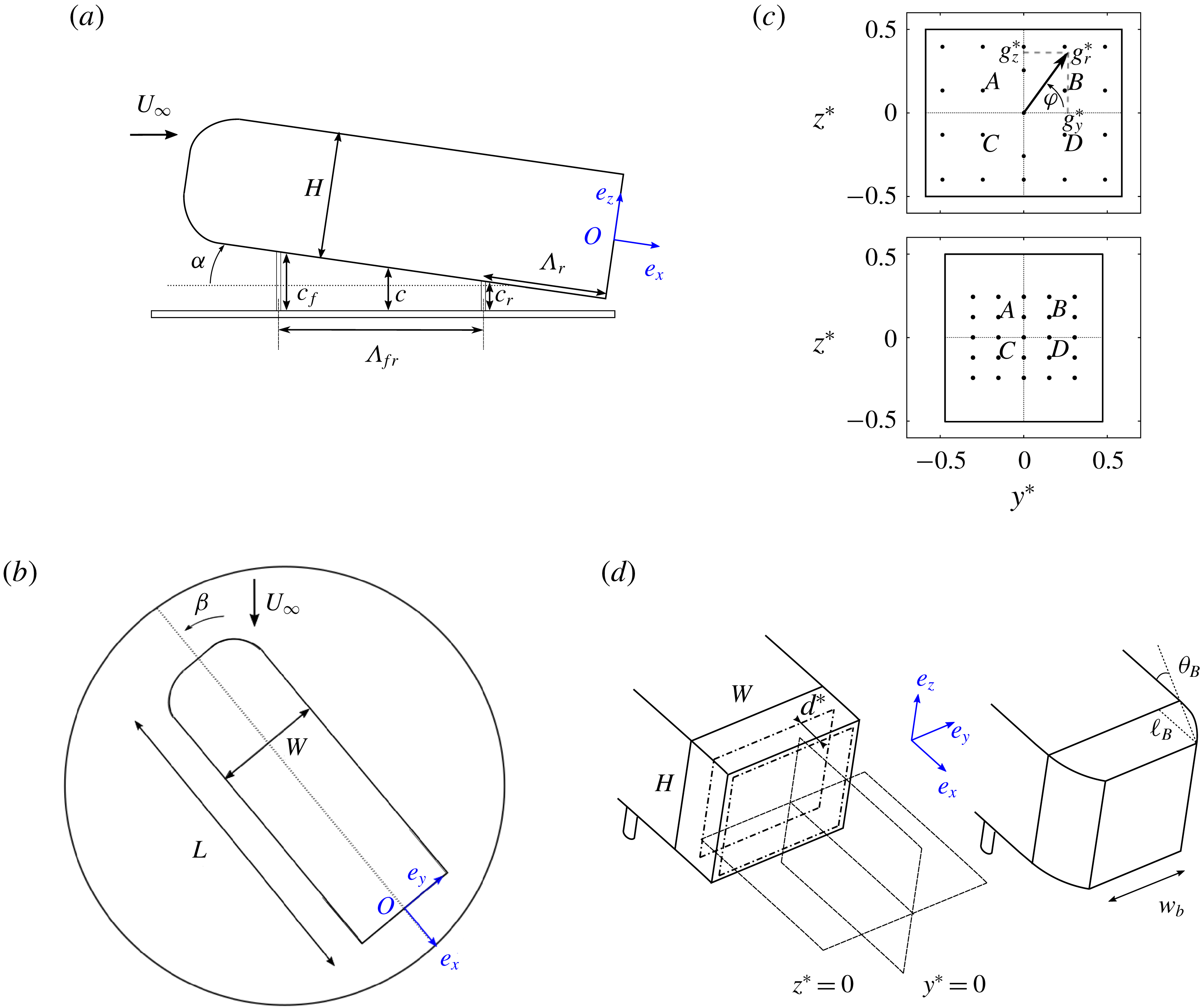
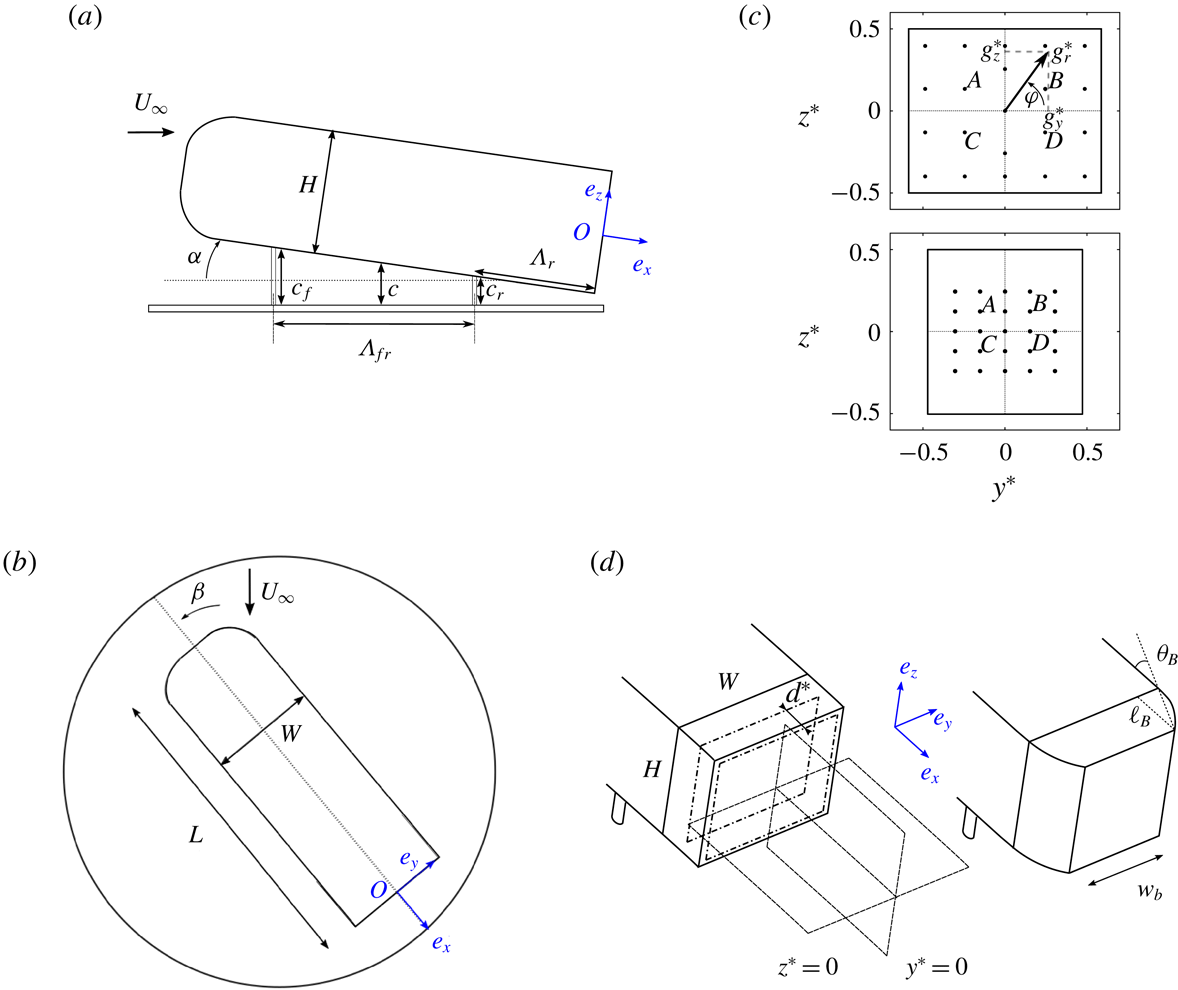
Figure 2. Experimental apparatus: schematic side view (a), top view (b) of the main body and rear views (c) of the square-back (top) and boat-tailed (bottom) body bases. In (c), the bases of the models are equipped with pressure sensors (black dots); the four points
 $A,B,C,D$
are used for calculation of the base pressure gradient
$A,B,C,D$
are used for calculation of the base pressure gradient
 $\hat{\boldsymbol{g}}^{\ast }$
(see text). Schematic view (d) of the square-back (left) and boat-tailed (right) after-bodies and representation of the fixed horizontal and vertical laser planes used for particle image velocimetry. They correspond to
$\hat{\boldsymbol{g}}^{\ast }$
(see text). Schematic view (d) of the square-back (left) and boat-tailed (right) after-bodies and representation of the fixed horizontal and vertical laser planes used for particle image velocimetry. They correspond to
 $y^{\ast }=0$
and
$y^{\ast }=0$
and
 $z^{\ast }=0$
for the aligned body case. The rectangular board that creates the cavity of the square-back after-body (when pushed inwards the body) is shown by the dashed rectangles in (d) for
$z^{\ast }=0$
for the aligned body case. The rectangular board that creates the cavity of the square-back after-body (when pushed inwards the body) is shown by the dashed rectangles in (d) for
 $d^{\ast }=0$
and
$d^{\ast }=0$
and
 $d^{\ast }=0.285$
.
$d^{\ast }=0.285$
.
The ground clearance
 $c^{\ast }$
(normal distance from the body to the ground) can be adjusted at the front within the range
$c^{\ast }$
(normal distance from the body to the ground) can be adjusted at the front within the range
 $c_{f}^{\ast }\in [0.050,0.170]$
and independently at the rear,
$c_{f}^{\ast }\in [0.050,0.170]$
and independently at the rear,
 $c_{r}^{\ast }$
within an identical range. These displacements are controlled by two Standa 8MVT188-20 translation stages placed inside the body and driven by a 8SMC4-USB controller. The repeatability and the precision of the ground clearance is, in non-dimensional value,
$c_{r}^{\ast }$
within an identical range. These displacements are controlled by two Standa 8MVT188-20 translation stages placed inside the body and driven by a 8SMC4-USB controller. The repeatability and the precision of the ground clearance is, in non-dimensional value,
 $\unicode[STIX]{x1D6FF}c^{\ast }\simeq 3.4\times 10^{-3}$
. The independence of each axis allows for a pitch angle given by
$\unicode[STIX]{x1D6FF}c^{\ast }\simeq 3.4\times 10^{-3}$
. The independence of each axis allows for a pitch angle given by
 $\tan \unicode[STIX]{x1D6FC}=(c_{f}-c_{r})/\unicode[STIX]{x1D6EC}_{fr}$
, where
$\tan \unicode[STIX]{x1D6FC}=(c_{f}-c_{r})/\unicode[STIX]{x1D6EC}_{fr}$
, where
 $\unicode[STIX]{x1D6EC}_{fr}$
is the wheelbase, kept constant owing to a sliding system mounted inside the body. The angle is counted positively in the clockwise orientation as shown in figure 2(a) and is varied in the range
$\unicode[STIX]{x1D6EC}_{fr}$
is the wheelbase, kept constant owing to a sliding system mounted inside the body. The angle is counted positively in the clockwise orientation as shown in figure 2(a) and is varied in the range
 $\unicode[STIX]{x1D6FC}\in [-1.5^{\circ },1.5^{\circ }]$
. The yaw angle
$\unicode[STIX]{x1D6FC}\in [-1.5^{\circ },1.5^{\circ }]$
. The yaw angle
 $\unicode[STIX]{x1D6FD}$
, defined in figure 2(b), can be adjusted by means of a rotating table mounted in the test section floor. This angle is counted following the direct orientation, the value
$\unicode[STIX]{x1D6FD}$
, defined in figure 2(b), can be adjusted by means of a rotating table mounted in the test section floor. This angle is counted following the direct orientation, the value
 $\unicode[STIX]{x1D6FD}=0^{\circ }$
corresponding to the body aligned with the incoming flow. It is considered aligned when, for a baseline ground clearance of
$\unicode[STIX]{x1D6FD}=0^{\circ }$
corresponding to the body aligned with the incoming flow. It is considered aligned when, for a baseline ground clearance of
 $c^{\ast }=0.168$
, the left and right orientations of the wake subjected to the
$c^{\ast }=0.168$
, the left and right orientations of the wake subjected to the
 $y$
-instability are equally explored for the duration of observation. The actual angle of the square-back body with respect to the wind tunnel is
$y$
-instability are equally explored for the duration of observation. The actual angle of the square-back body with respect to the wind tunnel is
 $\unicode[STIX]{x1D6FD}_{w}=-0.4^{\circ }$
, where
$\unicode[STIX]{x1D6FD}_{w}=-0.4^{\circ }$
, where
 $\unicode[STIX]{x1D6FD}_{w}$
is the angle between the wind tunnel longitudinal axis and the body. The yaw angle is varied in the range
$\unicode[STIX]{x1D6FD}_{w}$
is the angle between the wind tunnel longitudinal axis and the body. The yaw angle is varied in the range
 $\unicode[STIX]{x1D6FD}\in [-6.0^{\circ },6.0^{\circ }]$
.
$\unicode[STIX]{x1D6FD}\in [-6.0^{\circ },6.0^{\circ }]$
.
The experiments are carried out at the GIE-S2A in Montigny-le-Bretonneux (France) in a closed-loop model-scale wind tunnel dedicated to automotive aerodynamics. The incoming flow is a
 $3/4$
open jet with a cross-section of
$3/4$
open jet with a cross-section of
 $2.60~\text{m}\times 1.47~\text{m}$
. The plenum dimensions are
$2.60~\text{m}\times 1.47~\text{m}$
. The plenum dimensions are
 $9.30~\text{m}\times 6.60~\text{m}\times 4.15~\text{m}$
and the contraction ratio is
$9.30~\text{m}\times 6.60~\text{m}\times 4.15~\text{m}$
and the contraction ratio is
 $1:6$
. The thickness of the boundary layer is controlled by suction so that its displacement thickness equals
$1:6$
. The thickness of the boundary layer is controlled by suction so that its displacement thickness equals
 $\unicode[STIX]{x1D6FF}_{1}^{\ast }=1.0\times 10^{-2}$
at a distance
$\unicode[STIX]{x1D6FF}_{1}^{\ast }=1.0\times 10^{-2}$
at a distance
 $l_{0}^{\ast }=4.70$
upstream of the nose of the model. The flow inhomogeneity is lower than
$l_{0}^{\ast }=4.70$
upstream of the nose of the model. The flow inhomogeneity is lower than
 $0.5\,\%$
with an angular deviation smaller than
$0.5\,\%$
with an angular deviation smaller than
 $0.25^{\circ }$
at the considered regime. The free-stream velocity is set to
$0.25^{\circ }$
at the considered regime. The free-stream velocity is set to
 $U_{\infty }=20.0~\text{m}~\text{s}^{-1}$
and the temperature inside the vein is regulated at
$U_{\infty }=20.0~\text{m}~\text{s}^{-1}$
and the temperature inside the vein is regulated at
 $T_{\infty }=293.15~\text{K}$
with an uncertainty of less than
$T_{\infty }=293.15~\text{K}$
with an uncertainty of less than
 $0.1~\text{m}~\text{s}^{-1}$
and
$0.1~\text{m}~\text{s}^{-1}$
and
 $0.5~\text{K}$
respectively. Under those conditions, the corresponding Reynolds number is
$0.5~\text{K}$
respectively. Under those conditions, the corresponding Reynolds number is
 $Re=U_{\infty }H/\unicode[STIX]{x1D708}\simeq 4.0\times 10^{5}$
,
$Re=U_{\infty }H/\unicode[STIX]{x1D708}\simeq 4.0\times 10^{5}$
,
 $\unicode[STIX]{x1D708}$
being the air kinematic viscosity.
$\unicode[STIX]{x1D708}$
being the air kinematic viscosity.
2.2 Pressure measurements
Unsteady pressure is measured at the
 $N=21$
locations
$N=21$
locations
 $(y_{i}^{\ast },z_{i}^{\ast })$
indicated by the black dots at the base of the body in figure 2(c). The sampling frequency is set at
$(y_{i}^{\ast },z_{i}^{\ast })$
indicated by the black dots at the base of the body in figure 2(c). The sampling frequency is set at
 $200~\text{Hz}$
per channel with an accuracy of
$200~\text{Hz}$
per channel with an accuracy of
 $\pm 3.75~\text{Pa}$
and measurements are performed thanks to a Scanivalve ZOC22b pressure scanner connected to a Green Lake Engineering SmartZOC100 electronics. The low-pass cutoff frequency due to the tubing lengths between the pressure holes on the body and the pressure scanner is approximately
$\pm 3.75~\text{Pa}$
and measurements are performed thanks to a Scanivalve ZOC22b pressure scanner connected to a Green Lake Engineering SmartZOC100 electronics. The low-pass cutoff frequency due to the tubing lengths between the pressure holes on the body and the pressure scanner is approximately
 $50~\text{Hz}$
which is enough for the time resolution requested for the present study. The free-stream static pressure
$50~\text{Hz}$
which is enough for the time resolution requested for the present study. The free-stream static pressure
 $p_{\infty }$
, obtained directly from the facility, is used to compute the instantaneous pressure coefficient:
$p_{\infty }$
, obtained directly from the facility, is used to compute the instantaneous pressure coefficient:
 $$\begin{eqnarray}c_{p}(y^{\ast },z^{\ast },t^{\ast })=\frac{p(y^{\ast },z^{\ast },t^{\ast })-p_{\infty }}{\frac{1}{2}\unicode[STIX]{x1D70C}U_{\infty }^{2}},\end{eqnarray}$$
where
 $\unicode[STIX]{x1D70C}$
denotes the air density. The uncertainty on the pressure coefficient is approximately
$\unicode[STIX]{x1D70C}$
denotes the air density. The uncertainty on the pressure coefficient is approximately
 $2\times 10^{-3}$
.
$2\times 10^{-3}$
.
The instantaneous base suction coefficient
 $c_{b}(t^{\ast })$
is computed from the average on the
$c_{b}(t^{\ast })$
is computed from the average on the
 $N=21$
pressure taps at the base:
$N=21$
pressure taps at the base:
 $$\begin{eqnarray}c_{b}(t^{\ast })=-\frac{1}{N}\mathop{\sum }_{i=1}^{N}c_{p}(y_{i}^{\ast },z_{i}^{\ast },t^{\ast }).\end{eqnarray}$$
This coefficient is always positive in separated flow areas and follows similar trends as the total drag of the model (Roshko Reference Roshko1993).
Following the same experimental procedure as Grandemange et al. (Reference Grandemange, Gohlke and Cadot2013a
), four pressure sensors are used to compute the base pressure gradient which is representative of the instantaneous configuration of the wake. First, a horizontal component
 $g_{y}^{\ast }$
is computed as follows using the sensors marked
$g_{y}^{\ast }$
is computed as follows using the sensors marked
 $A$
,
$A$
,
 $B$
,
$B$
,
 $C$
and
$C$
and
 $D$
in figure 2(c):
$D$
in figure 2(c):
 $$\begin{eqnarray}g_{y}^{\ast }(t^{\ast })=\frac{1}{2}\times \left[\frac{c_{p}(y_{A}^{\ast },z_{A}^{\ast },t^{\ast })-c_{p}(y_{B}^{\ast },z_{B}^{\ast },t^{\ast })}{y_{A}^{\ast }-y_{B}^{\ast }}+\frac{c_{p}(y_{C}^{\ast },z_{C}^{\ast },t^{\ast })-c_{p}(y_{D}^{\ast },z_{D}^{\ast },t^{\ast })}{y_{C}^{\ast }-y_{D}^{\ast }}\right],\end{eqnarray}$$
where
 $y_{i}^{\ast }$
and
$y_{i}^{\ast }$
and
 $z_{i}^{\ast }$
stand for the coordinates of sensor
$z_{i}^{\ast }$
stand for the coordinates of sensor
 $i$
. The same process is repeated to compute the vertical component
$i$
. The same process is repeated to compute the vertical component
 $g_{z}^{\ast }$
using the pairs
$g_{z}^{\ast }$
using the pairs
 $(A,C)$
and
$(A,C)$
and
 $(B,D)$
. Finally, the complex base pressure gradient is obtained as
$(B,D)$
. Finally, the complex base pressure gradient is obtained as
 ${\hat{g}}^{\ast }=g_{y}^{\ast }+\text{i}g_{z}^{\ast }$
where
${\hat{g}}^{\ast }=g_{y}^{\ast }+\text{i}g_{z}^{\ast }$
where
 $\text{i}^{2}=-1$
. The modulus
$\text{i}^{2}=-1$
. The modulus
 $g_{r}^{\ast }=|{\hat{g}}^{\ast }|$
and the argument
$g_{r}^{\ast }=|{\hat{g}}^{\ast }|$
and the argument
 $\unicode[STIX]{x1D711}=\arg ({\hat{g}}^{\ast })$
of the polar form will be referred to as strength and phase of the base pressure gradient.
$\unicode[STIX]{x1D711}=\arg ({\hat{g}}^{\ast })$
of the polar form will be referred to as strength and phase of the base pressure gradient.
2.3 Aerodynamic load measurements
A six-component aerodynamics balance provided by Schencker GmbH and located beneath the wind tunnel floor is used to obtain time series of the aerodynamic forces at a sampling frequency set at
 $10~\text{Hz}$
. The model is connected to the balance by the four cylindrical supports. The forces
$10~\text{Hz}$
. The model is connected to the balance by the four cylindrical supports. The forces
 $(F_{x},F_{y},F_{z})$
are the components of the total aerodynamic load
$(F_{x},F_{y},F_{z})$
are the components of the total aerodynamic load
 $\boldsymbol{F}$
in the coordinate system described above. The uncertainty is
$\boldsymbol{F}$
in the coordinate system described above. The uncertainty is
 $0.3~\text{N}$
for the drag
$0.3~\text{N}$
for the drag
 $F_{x}$
and the side force
$F_{x}$
and the side force
 $F_{y}$
, whilst it is approximately
$F_{y}$
, whilst it is approximately
 $0.5~\text{N}$
for the lift
$0.5~\text{N}$
for the lift
 $F_{z}$
. The model frontal surface
$F_{z}$
. The model frontal surface
 $S$
is used to compute the force coefficients:
$S$
is used to compute the force coefficients:
 $$\begin{eqnarray}c_{i}=\frac{F_{i}}{\frac{1}{2}\unicode[STIX]{x1D70C}U_{\infty }^{2}S},\quad i=x,y,z,\end{eqnarray}$$
with a corresponding maximum uncertainty of
 $10^{-3}$
.
$10^{-3}$
.
2.4 Velocity measurements
Velocity fields are measured using two-dimensional particle image velocimetry (PIV) equipment. It is based on a dual pulse Nd:YAG laser (
 $200~\text{mJ}$
,
$200~\text{mJ}$
,
 $4~\text{ns}$
) creating a laser sheet whose thickness is
$4~\text{ns}$
) creating a laser sheet whose thickness is
 $5~\text{mm}$
and combined with a Dantec FlowSense EO
$5~\text{mm}$
and combined with a Dantec FlowSense EO
 $4~\text{MPx}$
CCD camera. Image pairs are shot at a rate of
$4~\text{MPx}$
CCD camera. Image pairs are shot at a rate of
 $4~\text{Hz}$
and
$4~\text{Hz}$
and
 $400$
snapshots are recorded. The interrogation window size is set to
$400$
snapshots are recorded. The interrogation window size is set to
 $32\times 32$
pixels, which corresponds to a physical size
$32\times 32$
pixels, which corresponds to a physical size
 $\unicode[STIX]{x1D6E5}_{y}^{\ast }\times \unicode[STIX]{x1D6E5}_{z}^{\ast }=0.017\times 0.017$
(or
$\unicode[STIX]{x1D6E5}_{y}^{\ast }\times \unicode[STIX]{x1D6E5}_{z}^{\ast }=0.017\times 0.017$
(or
 $\unicode[STIX]{x1D6E5}_{x}^{\ast }\times \unicode[STIX]{x1D6E5}_{z}^{\ast }=0.017\times 0.017$
for vertical planes) and with an overlap of
$\unicode[STIX]{x1D6E5}_{x}^{\ast }\times \unicode[STIX]{x1D6E5}_{z}^{\ast }=0.017\times 0.017$
for vertical planes) and with an overlap of
 $50\,\%$
. We investigate the two orthogonal planes fixed in the laboratory frame and located at the base of the body: a vertical one at mid-width that will be referred to as the
$50\,\%$
. We investigate the two orthogonal planes fixed in the laboratory frame and located at the base of the body: a vertical one at mid-width that will be referred to as the
 $y^{\ast }=0$
plane and a horizontal one that will be referred to as the
$y^{\ast }=0$
plane and a horizontal one that will be referred to as the
 $z^{\ast }=0$
plane. Both planes are shown in figure 2(d). Actually, when either a pitch or a yaw angle is introduced, the local coordinate system (
$z^{\ast }=0$
plane. Both planes are shown in figure 2(d). Actually, when either a pitch or a yaw angle is introduced, the local coordinate system (
 $\boldsymbol{e}_{x},\boldsymbol{e}_{y},\boldsymbol{e}_{z}$
) associated with the base in figure 2(d) will not coincide with the PIV measurements fields anymore. Since the considered angles are small (less than
$\boldsymbol{e}_{x},\boldsymbol{e}_{y},\boldsymbol{e}_{z}$
) associated with the base in figure 2(d) will not coincide with the PIV measurements fields anymore. Since the considered angles are small (less than
 $2^{\circ }$
), it was decided for the sake of simplicity to keep the same name for the space coordinates of the velocity fields. Using conventional notations, the PIV gives access to the field
$2^{\circ }$
), it was decided for the sake of simplicity to keep the same name for the space coordinates of the velocity fields. Using conventional notations, the PIV gives access to the field
 $\boldsymbol{u}_{xz}^{\ast }=u^{\ast }\boldsymbol{e}_{x}+w^{\ast }\boldsymbol{e}_{z}$
in the
$\boldsymbol{u}_{xz}^{\ast }=u^{\ast }\boldsymbol{e}_{x}+w^{\ast }\boldsymbol{e}_{z}$
in the
 $y^{\ast }=0$
plane and to
$y^{\ast }=0$
plane and to
 $\boldsymbol{u}_{xy}^{\ast }=u^{\ast }\boldsymbol{e}_{x}+v^{\ast }\boldsymbol{e}_{y}$
in the
$\boldsymbol{u}_{xy}^{\ast }=u^{\ast }\boldsymbol{e}_{x}+v^{\ast }\boldsymbol{e}_{y}$
in the
 $z^{\ast }=0$
plane.
$z^{\ast }=0$
plane.
2.5 Experimental protocol
Before each set of experiments, acquisitions of both the pressure and the forces are performed in no-wind conditions for a duration of
 $10$
s. The no-wind data are then averaged and subtracted from the force balance and pressure measurements. Regular tares are performed and zero values are checked to ensure accuracy, repeatability and reliability of the results.
$10$
s. The no-wind data are then averaged and subtracted from the force balance and pressure measurements. Regular tares are performed and zero values are checked to ensure accuracy, repeatability and reliability of the results.
Simultaneous base pressure and aerodynamic load measurements are recorded during
 $t=180~\text{s}$
(i.e.
$t=180~\text{s}$
(i.e.
 $t^{\ast }=12\,080$
in dimensionless units). Although this is not long enough to achieve complete statistical convergence (which in fact is a challenge to fulfil because of the long-time dynamics), this duration was chosen as a compromise that is sufficient to identify the most probable values.
$t^{\ast }=12\,080$
in dimensionless units). Although this is not long enough to achieve complete statistical convergence (which in fact is a challenge to fulfil because of the long-time dynamics), this duration was chosen as a compromise that is sufficient to identify the most probable values.
Since the paper focuses on the long-time dynamics of the unstable wake, base pressure and force balance data are low-pass filtered at
 $f_{c}=2~\text{Hz}$
(i.e.
$f_{c}=2~\text{Hz}$
(i.e.
 $f_{c}^{\ast }=0.03$
) by means of a moving average using a 0.5 s time window. As the natural cutoff frequency of the two measurements systems is larger, both sets of filtered data are comparable with an accurate frequency resolution.
$f_{c}^{\ast }=0.03$
) by means of a moving average using a 0.5 s time window. As the natural cutoff frequency of the two measurements systems is larger, both sets of filtered data are comparable with an accurate frequency resolution.
In addition to those measurements, PIV is performed in the two planes described in § 2.4. Base pressure measurements are made during the acquisition in order to perform conditional averaging based on synchronous measurements. For PIV measurements, snapshots are acquired during
 $t=100~\text{s}$
(i.e.
$t=100~\text{s}$
(i.e.
 $t^{\ast }=6711$
in dimensionless units).
$t^{\ast }=6711$
in dimensionless units).
3 Results
We recall that the superscript
 $^{\ast }$
indicates a quantity made non-dimensional using the uniform incoming flow velocity
$^{\ast }$
indicates a quantity made non-dimensional using the uniform incoming flow velocity
 $U_{\infty }$
and the body height
$U_{\infty }$
and the body height
 $H$
. Lower case letters
$H$
. Lower case letters
 $x$
are used for an instantaneous variable while upper case letters
$x$
are used for an instantaneous variable while upper case letters
 $X=\overline{x}$
denote the temporal averaging of the variable. The Reynolds notation is also used for fluctuations,
$X=\overline{x}$
denote the temporal averaging of the variable. The Reynolds notation is also used for fluctuations,
 $x(t)=X+x^{\prime }(t)$
for which the standard fluctuation is
$x(t)=X+x^{\prime }(t)$
for which the standard fluctuation is
 $X^{\prime }=\sqrt{\overline{{x^{\prime }}^{2}}}$
.
$X^{\prime }=\sqrt{\overline{{x^{\prime }}^{2}}}$
.
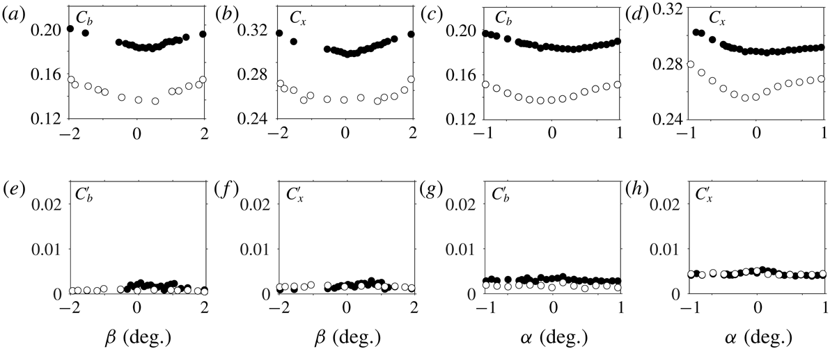
For the remainder of the paper, we will call the baseline the case where
 $\unicode[STIX]{x1D6FD}=\unicode[STIX]{x1D6FC}=0^{\circ }$
with a ground clearance
$\unicode[STIX]{x1D6FD}=\unicode[STIX]{x1D6FC}=0^{\circ }$
with a ground clearance
 $c^{\ast }=0.168$
. It is a similar configuration to that of Ahmed et al. (Reference Ahmed, Ramm and Faitin1984). We show in table 2 characteristic properties of the baseline without (
$c^{\ast }=0.168$
. It is a similar configuration to that of Ahmed et al. (Reference Ahmed, Ramm and Faitin1984). We show in table 2 characteristic properties of the baseline without (
 $d^{\ast }=0$
) and with the rear cavity (
$d^{\ast }=0$
) and with the rear cavity (
 $d^{\ast }=0.285$
). The drag coefficient of the baseline without the cavity lies within the range
$d^{\ast }=0.285$
). The drag coefficient of the baseline without the cavity lies within the range
 $0.25\leqslant C_{x}\leqslant 0.35$
reported in the literature (Ahmed et al.
Reference Ahmed, Ramm and Faitin1984; Barros et al.
Reference Barros, Ruiz, Borée and Noack2014; Volpe et al.
Reference Volpe, Devinant and Kourta2015; Evrard et al.
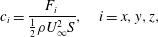
Reference Evrard, Cadot, Herbert, Ricot, Vigneron and Délery2016). For the square-back geometry, the large magnitude of the side force fluctuation
$0.25\leqslant C_{x}\leqslant 0.35$
reported in the literature (Ahmed et al.
Reference Ahmed, Ramm and Faitin1984; Barros et al.
Reference Barros, Ruiz, Borée and Noack2014; Volpe et al.
Reference Volpe, Devinant and Kourta2015; Evrard et al.
Reference Evrard, Cadot, Herbert, Ricot, Vigneron and Délery2016). For the square-back geometry, the large magnitude of the side force fluctuation
 $C_{y}^{\prime }=0.020$
(compared to those of the other components in table 2) reveals the
$C_{y}^{\prime }=0.020$
(compared to those of the other components in table 2) reveals the
 $y$
-instability through the bistable dynamics (Grandemange et al.
Reference Grandemange, Gohlke and Cadot2013b
; Evrard et al.
Reference Evrard, Cadot, Herbert, Ricot, Vigneron and Délery2016). The rear cavity produces a drag reduction of
$y$
-instability through the bistable dynamics (Grandemange et al.
Reference Grandemange, Gohlke and Cadot2013b
; Evrard et al.
Reference Evrard, Cadot, Herbert, Ricot, Vigneron and Délery2016). The rear cavity produces a drag reduction of
 $9.7\,\%$
together with strong attenuation of the side force fluctuation in conformity with Evrard et al. (Reference Evrard, Cadot, Herbert, Ricot, Vigneron and Délery2016), Lucas et al. (Reference Lucas, Cadot, Herbert, Parpais and Délery2017).
$9.7\,\%$
together with strong attenuation of the side force fluctuation in conformity with Evrard et al. (Reference Evrard, Cadot, Herbert, Ricot, Vigneron and Délery2016), Lucas et al. (Reference Lucas, Cadot, Herbert, Parpais and Délery2017).
The first part of the results in § 3.1 will consider the square-back geometry with the aim of performing sensitivity analyses of the
 $y$
-instability. While the presence of a
$y$
-instability. While the presence of a
 $y$
-instability is easily detectable because of the reflectional symmetry breaking in the
$y$
-instability is easily detectable because of the reflectional symmetry breaking in the
 $y$
-direction, it is much more difficult to diagnose the
$y$
-direction, it is much more difficult to diagnose the
 $z$
-instability. Actually there is no reflectional symmetry to break in the
$z$
-instability. Actually there is no reflectional symmetry to break in the
 $z$
-direction because of the ground proximity and body supports. There is also no obvious reason to observe bistability that would unambiguously reveal the presence of the
$z$
-direction because of the ground proximity and body supports. There is also no obvious reason to observe bistability that would unambiguously reveal the presence of the
 $z$
-instability. The second part of the results in § 3.2 will consider the boat-tailed geometry in order to investigate sensitivity analyses of the
$z$
-instability. The second part of the results in § 3.2 will consider the boat-tailed geometry in order to investigate sensitivity analyses of the
 $z$
-instability.
$z$
-instability.
Table 2. Characteristic mean and fluctuating coefficients for baseline configurations defined as
 $c^{\ast }=0.168,\unicode[STIX]{x1D6FC}=0^{\circ },\unicode[STIX]{x1D6FD}=0^{\circ }$
without (
$c^{\ast }=0.168,\unicode[STIX]{x1D6FC}=0^{\circ },\unicode[STIX]{x1D6FD}=0^{\circ }$
without (
 $d^{\ast }=0$
) and with (
$d^{\ast }=0$
) and with (
 $d^{\ast }=0.285$
) the rear cavity for the square-back geometry (
$d^{\ast }=0.285$
) the rear cavity for the square-back geometry (
 $w_{b}^{\ast }=1.174$
) and for the boat-tailed geometry (
$w_{b}^{\ast }=1.174$
) and for the boat-tailed geometry (
 $w_{b}^{\ast }=0.940$
).
$w_{b}^{\ast }=0.940$
).

3.1 The
 $y$
-instability
$y$
-instability

This section presents results about the square-back geometry only. In § 3.1.1, we show sensitivity maps of the base pressure gradient responses to variations of the ground clearance
 $c^{\ast }$
, the yaw angle
$c^{\ast }$
, the yaw angle
 $\unicode[STIX]{x1D6FD}$
and the pitch angle
$\unicode[STIX]{x1D6FD}$
and the pitch angle
 $\unicode[STIX]{x1D6FC}$
around the baseline. The responses are assessed through the statistics of the base pressure gradient
$\unicode[STIX]{x1D6FC}$
around the baseline. The responses are assessed through the statistics of the base pressure gradient
 ${\hat{g}}^{\ast }$
considering each component of both coordinate systems
${\hat{g}}^{\ast }$
considering each component of both coordinate systems
 $(g_{y}^{\ast },g_{z}^{\ast })$
and
$(g_{y}^{\ast },g_{z}^{\ast })$
and
 $(g_{r}^{\ast },\unicode[STIX]{x1D711})$
by representing its probability density function
$(g_{r}^{\ast },\unicode[STIX]{x1D711})$
by representing its probability density function
 $f$
normalized by its most probable value. The resulting plots are four two-dimensional sensitivity maps for each of the three geometrical configurations varying the geometrical parameter
$f$
normalized by its most probable value. The resulting plots are four two-dimensional sensitivity maps for each of the three geometrical configurations varying the geometrical parameter
 $q=c^{\ast },\unicode[STIX]{x1D6FC}$
or
$q=c^{\ast },\unicode[STIX]{x1D6FC}$
or
 $\unicode[STIX]{x1D6FD}:f(q,g_{y}^{\ast })$
,
$\unicode[STIX]{x1D6FD}:f(q,g_{y}^{\ast })$
,
 $f(q,g_{z}^{\ast })$
,
$f(q,g_{z}^{\ast })$
,
 $f(q,g_{r}^{\ast })$
and
$f(q,g_{r}^{\ast })$
and
 $f(q,\unicode[STIX]{x1D711})$
. The wake dynamics and topology are then investigated for chosen specific configurations reflecting all situations. In § 3.1.2, the procedure is repeated with the rear cavity. In § 3.1.3, the aerodynamic force sensitivity is examined and compared to the base pressure gradient contribution with and without the rear cavity.
$f(q,\unicode[STIX]{x1D711})$
. The wake dynamics and topology are then investigated for chosen specific configurations reflecting all situations. In § 3.1.2, the procedure is repeated with the rear cavity. In § 3.1.3, the aerodynamic force sensitivity is examined and compared to the base pressure gradient contribution with and without the rear cavity.
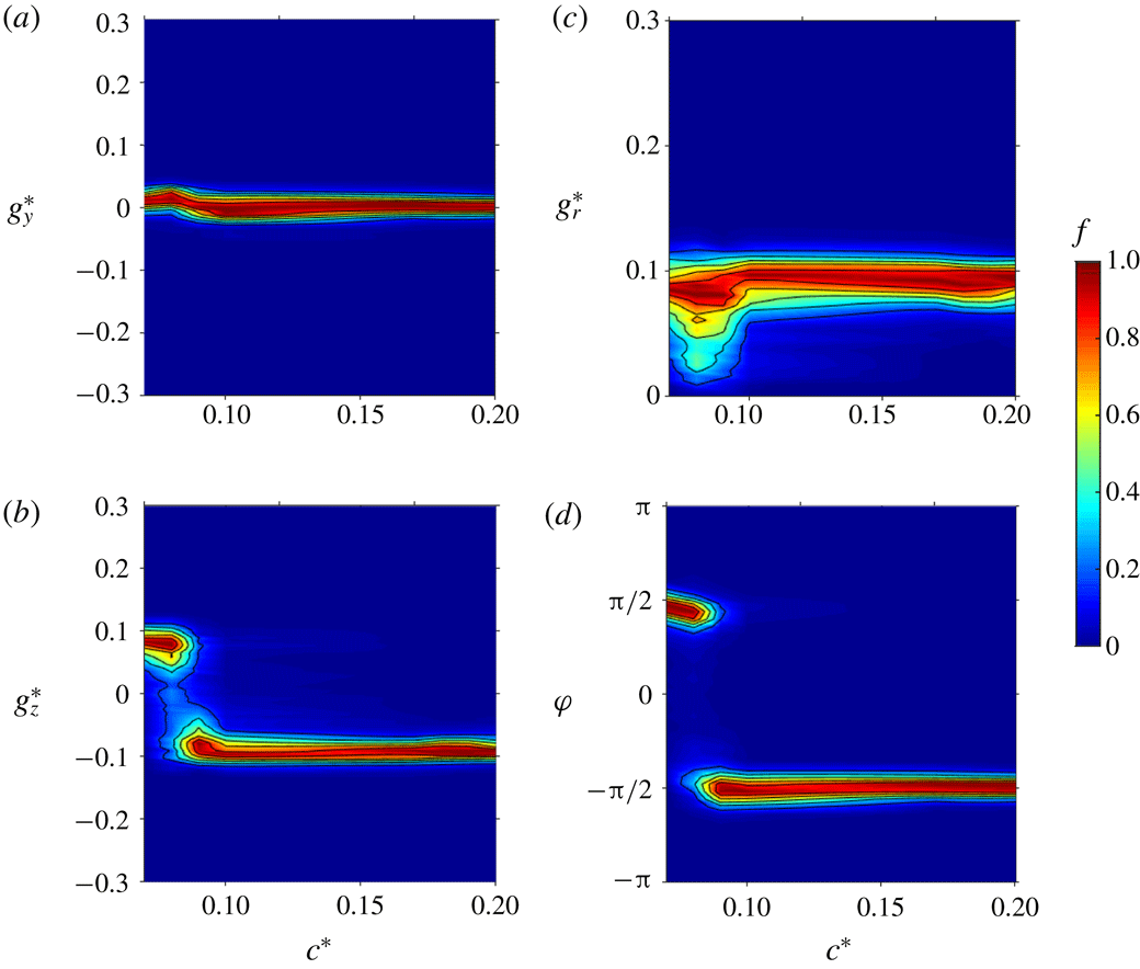
3.1.1 Wake sensitivity to the body clearance and inclinations
The four sensitivity maps of the base pressure gradient due to the variation of the ground clearance
 $c^{\ast }$
are shown in figure 3(a,b) for the Cartesian components and figure 3(c,d) for the polar form. When the body is gradually raised in figure 3(a), the most probable branch for
$c^{\ast }$
are shown in figure 3(a,b) for the Cartesian components and figure 3(c,d) for the polar form. When the body is gradually raised in figure 3(a), the most probable branch for
 $g_{y}^{\ast }$
observed for
$g_{y}^{\ast }$
observed for
 $c^{\ast }<0.080$
bifurcates in two symmetrical branches resulting from an instability. This was already fully described by Grandemange et al. (Reference Grandemange, Gohlke and Cadot2013a
), Cadot et al. (Reference Cadot, Evrard and Pastur2015) showing that the ground proximity suppresses the instability towards a symmetric wake through a pitchfork bifurcation. The region we consider is for large values of
$c^{\ast }<0.080$
bifurcates in two symmetrical branches resulting from an instability. This was already fully described by Grandemange et al. (Reference Grandemange, Gohlke and Cadot2013a
), Cadot et al. (Reference Cadot, Evrard and Pastur2015) showing that the ground proximity suppresses the instability towards a symmetric wake through a pitchfork bifurcation. The region we consider is for large values of
 $c^{\ast }$
for which the wake dynamics is dominated by the stochastic exploration of the two symmetric branches. Independently of the sign of
$c^{\ast }$
for which the wake dynamics is dominated by the stochastic exploration of the two symmetric branches. Independently of the sign of
 $g_{y}^{\ast }$
(i.e. the random switching dynamics) the permanent asymmetry introduced by the symmetry-breaking (SB) modes can be seen in the modulus
$g_{y}^{\ast }$
(i.e. the random switching dynamics) the permanent asymmetry introduced by the symmetry-breaking (SB) modes can be seen in the modulus
 $g_{r}^{\ast }$
displayed in figure 3(c). The modulus saturates to a constant value when
$g_{r}^{\ast }$
displayed in figure 3(c). The modulus saturates to a constant value when
 $c^{\ast }>c_{S}^{\ast }\simeq 0.105$
as shown in the figures. The regime
$c^{\ast }>c_{S}^{\ast }\simeq 0.105$
as shown in the figures. The regime
 $c^{\ast }>c_{S}^{\ast }$
corresponds to the unstable wake due to the
$c^{\ast }>c_{S}^{\ast }$
corresponds to the unstable wake due to the
 $y$
- or
$y$
- or
 $z$
-instability (Grandemange et al.
Reference Grandemange, Gohlke and Cadot2013a
), and will be referred to as the saturated regime throughout. The interesting result is that, whilst the vertical base pressure gradient
$z$
-instability (Grandemange et al.
Reference Grandemange, Gohlke and Cadot2013a
), and will be referred to as the saturated regime throughout. The interesting result is that, whilst the vertical base pressure gradient
 $g_{z}^{\ast }$
decreases significantly, the gradient modulus
$g_{z}^{\ast }$
decreases significantly, the gradient modulus
 $g_{r}^{\ast }$
remains constant and corresponds to a change in the gradient orientation
$g_{r}^{\ast }$
remains constant and corresponds to a change in the gradient orientation
 $\unicode[STIX]{x1D711}$
.
$\unicode[STIX]{x1D711}$
.

Figure 3. Base pressure gradient response to a variation of the ground clearance
 $c^{\ast }$
for the square-back body. Sensitivity maps (a)
$c^{\ast }$
for the square-back body. Sensitivity maps (a)
 $f(c^{\ast },g_{y}^{\ast })$
, (b)
$f(c^{\ast },g_{y}^{\ast })$
, (b)
 $f(c^{\ast },g_{z}^{\ast })$
, (c)
$f(c^{\ast },g_{z}^{\ast })$
, (c)
 $f(c^{\ast },g_{r}^{\ast })$
and (d)
$f(c^{\ast },g_{r}^{\ast })$
and (d)
 $f(c^{\ast },\unicode[STIX]{x1D711})$
. The clearance
$f(c^{\ast },\unicode[STIX]{x1D711})$
. The clearance
 $c_{S}^{\ast }\simeq 0.105$
is defined as the threshold from which the instability is saturated. See discussion § 4.1 for white symbols.
$c_{S}^{\ast }\simeq 0.105$
is defined as the threshold from which the instability is saturated. See discussion § 4.1 for white symbols.

Figure 4. Base pressure gradient response to variations of the yaw angle
 $\unicode[STIX]{x1D6FD}$
for the square-back body. Sensitivity maps (a)
$\unicode[STIX]{x1D6FD}$
for the square-back body. Sensitivity maps (a)
 $f(\unicode[STIX]{x1D6FD},g_{y}^{\ast })$
, (b)
$f(\unicode[STIX]{x1D6FD},g_{y}^{\ast })$
, (b)
 $f(\unicode[STIX]{x1D6FD},g_{z}^{\ast })$
, (c)
$f(\unicode[STIX]{x1D6FD},g_{z}^{\ast })$
, (c)
 $f(\unicode[STIX]{x1D6FD},g_{r}^{\ast })$
and (d)
$f(\unicode[STIX]{x1D6FD},g_{r}^{\ast })$
and (d)
 $f(\unicode[STIX]{x1D6FD},\unicode[STIX]{x1D711})$
. See discussion § 4.1 for white symbols.
$f(\unicode[STIX]{x1D6FD},\unicode[STIX]{x1D711})$
. See discussion § 4.1 for white symbols.

Figure 5. Base pressure gradient response to variations of the pitch angle
 $\unicode[STIX]{x1D6FC}$
for the square-back body. Sensitivity maps (a)
$\unicode[STIX]{x1D6FC}$
for the square-back body. Sensitivity maps (a)
 $f(\unicode[STIX]{x1D6FC},g_{y}^{\ast })$
, (b)
$f(\unicode[STIX]{x1D6FC},g_{y}^{\ast })$
, (b)
 $f(\unicode[STIX]{x1D6FC},g_{z}^{\ast })$
, (c)
$f(\unicode[STIX]{x1D6FC},g_{z}^{\ast })$
, (c)
 $f(\unicode[STIX]{x1D6FC},g_{r}^{\ast })$
and (d)
$f(\unicode[STIX]{x1D6FC},g_{r}^{\ast })$
and (d)
 $f(\unicode[STIX]{x1D6FC},\unicode[STIX]{x1D711})$
. See discussion § 4.1 for white symbols.
$f(\unicode[STIX]{x1D6FC},\unicode[STIX]{x1D711})$
. See discussion § 4.1 for white symbols.

Figure 6. Modulus
 $g_{r\unicode[STIX]{x1D6FC}}^{\ast }(t^{\ast })$
and phase
$g_{r\unicode[STIX]{x1D6FC}}^{\ast }(t^{\ast })$
and phase
 $\unicode[STIX]{x1D711}_{\unicode[STIX]{x1D6FC}}(t^{\ast })$
time series (left) of the base pressure gradient for the square-back body. Corresponding probability density functions (PDFs) (right) for (a) nose-down
$\unicode[STIX]{x1D711}_{\unicode[STIX]{x1D6FC}}(t^{\ast })$
time series (left) of the base pressure gradient for the square-back body. Corresponding probability density functions (PDFs) (right) for (a) nose-down
 $\unicode[STIX]{x1D6FC}=-1^{\circ }$
, (b) baseline
$\unicode[STIX]{x1D6FC}=-1^{\circ }$
, (b) baseline
 $\unicode[STIX]{x1D6FC}=0^{\circ }$
and (c) nose-up
$\unicode[STIX]{x1D6FC}=0^{\circ }$
and (c) nose-up
 $\unicode[STIX]{x1D6FC}=+1^{\circ }$
. The smooth red lines superimposed on the PDFs (
$\unicode[STIX]{x1D6FC}=+1^{\circ }$
. The smooth red lines superimposed on the PDFs (
 $g_{r}^{\ast }$
) in (a), (b) and (c) are best fits of Rigas et al.’s (Reference Rigas, Morgans, Brackston and Morrison2015) PDF model; the three parameters of the fit are not given.
$g_{r}^{\ast }$
) in (a), (b) and (c) are best fits of Rigas et al.’s (Reference Rigas, Morgans, Brackston and Morrison2015) PDF model; the three parameters of the fit are not given.
For the next two series of experiments concerning yaw and pitch sensitivities, we will consider small variations of the inclination around the baseline (see table 2). The baseline has most probable gradients that take phase values very close to
 $\unicode[STIX]{x1D711}\simeq 0$
or
$\unicode[STIX]{x1D711}\simeq 0$
or
 $\unicode[STIX]{x03C0}$
and a modulus
$\unicode[STIX]{x03C0}$
and a modulus
 $g_{r}^{\ast }\simeq 0.187$
obtained in figure 3(c).
$g_{r}^{\ast }\simeq 0.187$
obtained in figure 3(c).
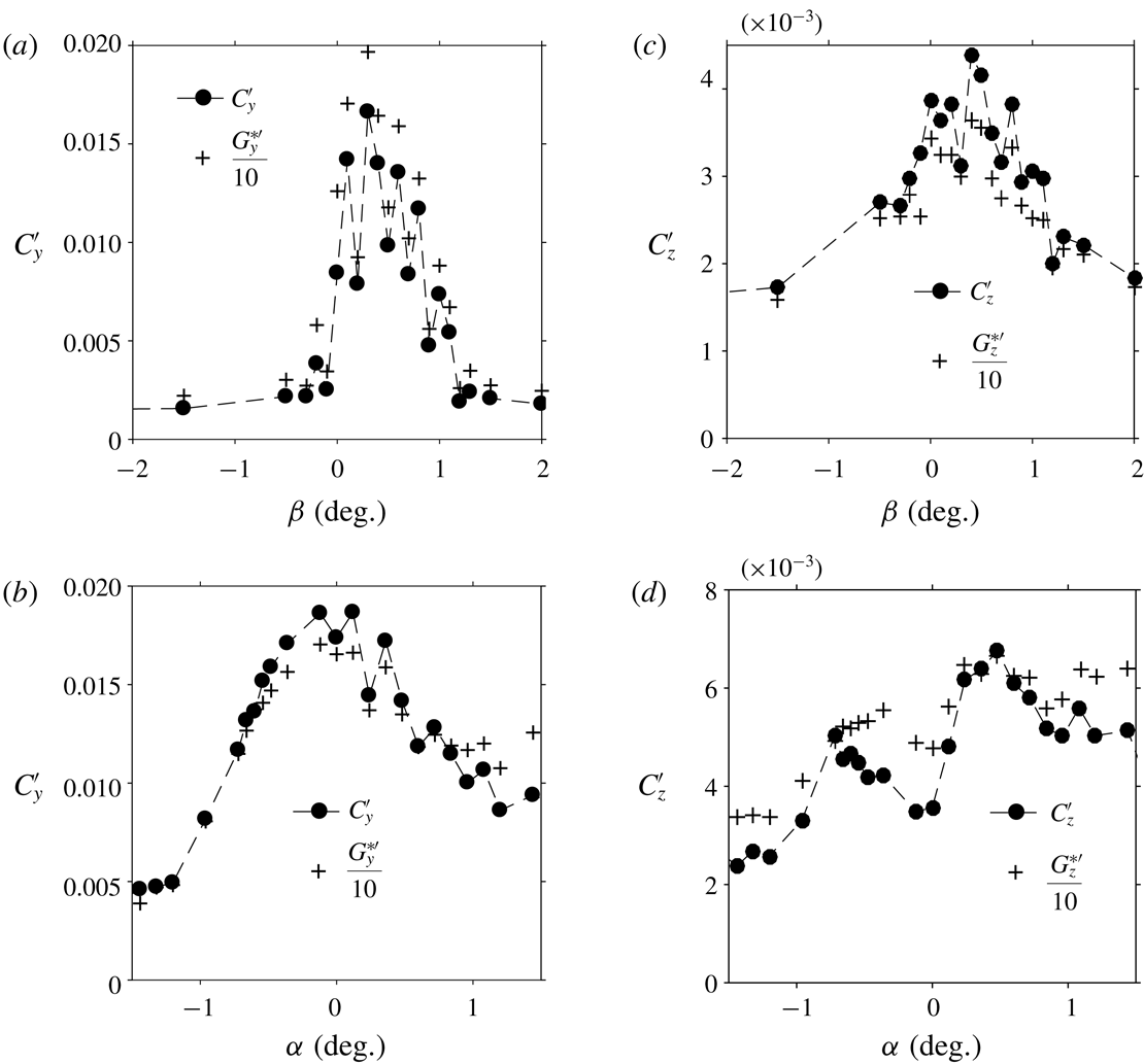
The sensitivity analysis to small variations of the yaw angle
 $\unicode[STIX]{x1D6FD}$
with a fixed ground clearance
$\unicode[STIX]{x1D6FD}$
with a fixed ground clearance
 $c^{\ast }=0.168$
and pitch
$c^{\ast }=0.168$
and pitch
 $\unicode[STIX]{x1D6FC}=0^{\circ }$
is shown in figure 4. The main result observed in figure 4(a) and previously reported in Cadot et al. (Reference Cadot, Evrard and Pastur2015), Volpe et al. (Reference Volpe, Devinant and Kourta2015), Evrard et al. (Reference Evrard, Cadot, Herbert, Ricot, Vigneron and Délery2016) is a discontinuous transition between two opposite branches of
$\unicode[STIX]{x1D6FC}=0^{\circ }$
is shown in figure 4. The main result observed in figure 4(a) and previously reported in Cadot et al. (Reference Cadot, Evrard and Pastur2015), Volpe et al. (Reference Volpe, Devinant and Kourta2015), Evrard et al. (Reference Evrard, Cadot, Herbert, Ricot, Vigneron and Délery2016) is a discontinuous transition between two opposite branches of
 $g_{y}^{\ast }$
which implies a phase jump (figure 4
d) between values close to
$g_{y}^{\ast }$
which implies a phase jump (figure 4
d) between values close to
 $0$
and
$0$
and
 $\unicode[STIX]{x03C0}$
. Nevertheless, this transition occurs with a fairly constant modulus
$\unicode[STIX]{x03C0}$
. Nevertheless, this transition occurs with a fairly constant modulus
 $g_{r}^{\ast }$
as shown in figure 4(c). The vertical component
$g_{r}^{\ast }$
as shown in figure 4(c). The vertical component
 $g_{z}^{\ast }$
in figure 4(b) has a slight, unexpected affine variation with the yaw which is likely to be due to an imperfection of the set-up, coming from multiple sources such as wind inhomogeneity, non-zero roll angle and cable passage behind the rear right-hand side cylindrical support. Because of the constant modulus, the set-up imperfections affect slightly the phase
$g_{z}^{\ast }$
in figure 4(b) has a slight, unexpected affine variation with the yaw which is likely to be due to an imperfection of the set-up, coming from multiple sources such as wind inhomogeneity, non-zero roll angle and cable passage behind the rear right-hand side cylindrical support. Because of the constant modulus, the set-up imperfections affect slightly the phase
 $\unicode[STIX]{x1D711}$
(figure 3
d) which slightly deviates from
$\unicode[STIX]{x1D711}$
(figure 3
d) which slightly deviates from
 $\unicode[STIX]{x1D711}_{0}=0$
or
$\unicode[STIX]{x1D711}_{0}=0$
or
 $\unicode[STIX]{x1D711}_{0}=\unicode[STIX]{x03C0}$
.
$\unicode[STIX]{x1D711}_{0}=\unicode[STIX]{x03C0}$
.
We now turn to the sensitivity to the pitch angle
 $\unicode[STIX]{x1D6FC}$
. The yaw angle is set to
$\unicode[STIX]{x1D6FC}$
. The yaw angle is set to
 $\unicode[STIX]{x1D6FD}=0^{\circ }$
and the front and rear ground clearances are adjusted for a given pitch but keeping
$\unicode[STIX]{x1D6FD}=0^{\circ }$
and the front and rear ground clearances are adjusted for a given pitch but keeping
 $c^{\ast }=(c_{f}^{\ast }+c_{r}^{\ast })/2=0.168$
in order to recover the baseline when
$c^{\ast }=(c_{f}^{\ast }+c_{r}^{\ast })/2=0.168$
in order to recover the baseline when
 $c_{f}^{\ast }=c_{r}^{\ast }$
. The sensitivity results of the base pressure gradient are shown in figure 5. Looking at figure 5(a), which shows the sensitivity of the horizontal gradient component
$c_{f}^{\ast }=c_{r}^{\ast }$
. The sensitivity results of the base pressure gradient are shown in figure 5. Looking at figure 5(a), which shows the sensitivity of the horizontal gradient component
 $g_{y}^{\ast }$
, we can distinguish three regimes. At large nose-down, for
$g_{y}^{\ast }$
, we can distinguish three regimes. At large nose-down, for
 $\unicode[STIX]{x1D6FC}\lesssim -0.75^{\circ }$
, there is a single branch located around
$\unicode[STIX]{x1D6FC}\lesssim -0.75^{\circ }$
, there is a single branch located around
 $g_{y}^{\ast }=0$
, which bifurcates in two opposite branches in the range
$g_{y}^{\ast }=0$
, which bifurcates in two opposite branches in the range
 $-0.75^{\circ }\lesssim \unicode[STIX]{x1D6FC}\lesssim 0.5^{\circ }$
. In the last regime with nose-up, for which
$-0.75^{\circ }\lesssim \unicode[STIX]{x1D6FC}\lesssim 0.5^{\circ }$
. In the last regime with nose-up, for which
 $\unicode[STIX]{x1D6FC}\gtrsim 0.5^{\circ }$
, the horizontal component varies almost uniformly in a wide range
$\unicode[STIX]{x1D6FC}\gtrsim 0.5^{\circ }$
, the horizontal component varies almost uniformly in a wide range
 $|g_{y}^{\ast }|\lesssim 0.2$
.
$|g_{y}^{\ast }|\lesssim 0.2$
.
The effect of the pitch on the vertical gradient component
 $g_{z}^{\ast }$
is shown in figure 5(b). It displays a monotonic variation with the pitch angle in the range
$g_{z}^{\ast }$
is shown in figure 5(b). It displays a monotonic variation with the pitch angle in the range
 $-0.75^{\circ }\lesssim \unicode[STIX]{x1D6FC}\lesssim 0.5^{\circ }$
coincidently with the two branches observed for
$-0.75^{\circ }\lesssim \unicode[STIX]{x1D6FC}\lesssim 0.5^{\circ }$
coincidently with the two branches observed for
 $g_{y}^{\ast }$
. Apart from this range, the vertical component is saturated to extreme values. Although these three regimes are very different, the modulus shown in figure 5(c) displays an almost symmetric evolution, with decreases on both sides of the maximum. In the third regime, the phase is unlocked in the
$g_{y}^{\ast }$
. Apart from this range, the vertical component is saturated to extreme values. Although these three regimes are very different, the modulus shown in figure 5(c) displays an almost symmetric evolution, with decreases on both sides of the maximum. In the third regime, the phase is unlocked in the
 $[-\unicode[STIX]{x03C0},0]$
interval with a rather uniform exploration (figure 5
d), unlike nose-down regimes. This different behaviour is attributed to the wall proximity at the trailing edge which has a major effect on the base flow in nose-up configurations.
$[-\unicode[STIX]{x03C0},0]$
interval with a rather uniform exploration (figure 5
d), unlike nose-down regimes. This different behaviour is attributed to the wall proximity at the trailing edge which has a major effect on the base flow in nose-up configurations.
Most importantly, a similar conclusion as for the ground clearance and the yaw experiments can be drawn. The small pitch angle variation produces a component
 $g_{z}^{\ast }$
of the vertical pressure gradient. The modulus
$g_{z}^{\ast }$
of the vertical pressure gradient. The modulus
 $g_{r}^{\ast }$
is slightly modulated, maximum for horizontal orientation and minimum for vertical one.
$g_{r}^{\ast }$
is slightly modulated, maximum for horizontal orientation and minimum for vertical one.

Figure 7. Cross-sections of the mean velocity field of the square-back body visualized using streamlines superimposed on the modulus of the components in the vertical plane
 $(x^{\ast },z^{\ast })$
(a,c,e) and horizontal plane
$(x^{\ast },z^{\ast })$
(a,c,e) and horizontal plane
 $(x^{\ast },y^{\ast })$
(b,d,f) for (a,b) nose-down
$(x^{\ast },y^{\ast })$
(b,d,f) for (a,b) nose-down
 $\unicode[STIX]{x1D6FC}=-1^{\circ }$
, (c,d) baseline
$\unicode[STIX]{x1D6FC}=-1^{\circ }$
, (c,d) baseline
 $\unicode[STIX]{x1D6FC}=0^{\circ }$
(
$\unicode[STIX]{x1D6FC}=0^{\circ }$
(
 $P$
state, see text) and (e,f) nose-up
$P$
state, see text) and (e,f) nose-up
 $\unicode[STIX]{x1D6FC}=+1^{\circ }$
.
$\unicode[STIX]{x1D6FC}=+1^{\circ }$
.
The wake dynamics of the four configurations of the base pressure gradient orientations: vertical positive, horizontal (positive and negative) and vertical negative is now respectively investigated through the pitch angles
 $\unicode[STIX]{x1D6FC}=-1^{\circ }$
,
$\unicode[STIX]{x1D6FC}=-1^{\circ }$
,
 $\unicode[STIX]{x1D6FC}=0^{\circ }$
and
$\unicode[STIX]{x1D6FC}=0^{\circ }$
and
 $\unicode[STIX]{x1D6FC}=1^{\circ }$
. We show the corresponding time series of the gradient modulus
$\unicode[STIX]{x1D6FC}=1^{\circ }$
. We show the corresponding time series of the gradient modulus
 $g_{r\unicode[STIX]{x1D6FC}}^{\ast }(t^{\ast })$
and phase
$g_{r\unicode[STIX]{x1D6FC}}^{\ast }(t^{\ast })$
and phase
 $\unicode[STIX]{x1D711}_{\unicode[STIX]{x1D6FC}}(t^{\ast })$
in figure 6. The nose-down at
$\unicode[STIX]{x1D711}_{\unicode[STIX]{x1D6FC}}(t^{\ast })$
in figure 6. The nose-down at
 $\unicode[STIX]{x1D6FC}=-1^{\circ }$
in figure 6(a) clearly depicts a phase lock-in for
$\unicode[STIX]{x1D6FC}=-1^{\circ }$
in figure 6(a) clearly depicts a phase lock-in for
 $\unicode[STIX]{x1D711}_{-1^{\circ }}(t^{\ast })$
at
$\unicode[STIX]{x1D711}_{-1^{\circ }}(t^{\ast })$
at
 $\unicode[STIX]{x03C0}/2$
with turbulent fluctuations. When the pitch is set to zero (baseline configuration), the phase dynamics in figure 6(b) consists of random jumps of
$\unicode[STIX]{x03C0}/2$
with turbulent fluctuations. When the pitch is set to zero (baseline configuration), the phase dynamics in figure 6(b) consists of random jumps of
 $\unicode[STIX]{x03C0}$
and elsewhere to very long-time duration of typically
$\unicode[STIX]{x03C0}$
and elsewhere to very long-time duration of typically
 $\unicode[STIX]{x1D6FF}t^{\ast }=1000$
of phase lock-in at
$\unicode[STIX]{x1D6FF}t^{\ast }=1000$
of phase lock-in at
 $0$
and
$0$
and
 $-\unicode[STIX]{x03C0}$
. This long-time bistable dynamics was fully described in Grandemange et al. (Reference Grandemange, Gohlke and Cadot2013b
) using Cartesian coordinates for the gradient. It is worth mentioning that the dynamics is not only mainly made of phase jumps, since some events of the phase
$-\unicode[STIX]{x03C0}$
. This long-time bistable dynamics was fully described in Grandemange et al. (Reference Grandemange, Gohlke and Cadot2013b
) using Cartesian coordinates for the gradient. It is worth mentioning that the dynamics is not only mainly made of phase jumps, since some events of the phase
 $\unicode[STIX]{x1D711}_{0^{\circ }}$
occur around
$\unicode[STIX]{x1D711}_{0^{\circ }}$
occur around
 $-\unicode[STIX]{x03C0}/2$
with long-time evolution related to phase drift or wake rotation (see for instance within the time interval
$-\unicode[STIX]{x03C0}/2$
with long-time evolution related to phase drift or wake rotation (see for instance within the time interval
 $[1;2]\times 10^{3}$
in figure 6
b). For the nose-up case, there is no phase lock-in but large phase fluctuations associated with random wake rotations exploring the range
$[1;2]\times 10^{3}$
in figure 6
b). For the nose-up case, there is no phase lock-in but large phase fluctuations associated with random wake rotations exploring the range
 $[-\unicode[STIX]{x03C0},0]$
with some phase jumps like the one observed at
$[-\unicode[STIX]{x03C0},0]$
with some phase jumps like the one observed at
 $t^{\ast }=4.5\times 10^{3}$
in figure 6(c). There are obviously some similarities with the diffusive dynamics of the turbulent axisymmetric wake of Rigas et al. (Reference Rigas, Oxlade, Morgans and Morrison2014, Reference Rigas, Morgans, Brackston and Morrison2015), the main difference being the random walk of the phase that is bounded. Since the modulus is decoupled from the phase in Rigas et al.’s (Reference Rigas, Morgans, Brackston and Morrison2015) model, it is possible to present a best fit of the statistics of the gradient modulus
$t^{\ast }=4.5\times 10^{3}$
in figure 6(c). There are obviously some similarities with the diffusive dynamics of the turbulent axisymmetric wake of Rigas et al. (Reference Rigas, Oxlade, Morgans and Morrison2014, Reference Rigas, Morgans, Brackston and Morrison2015), the main difference being the random walk of the phase that is bounded. Since the modulus is decoupled from the phase in Rigas et al.’s (Reference Rigas, Morgans, Brackston and Morrison2015) model, it is possible to present a best fit of the statistics of the gradient modulus
 $g_{r}^{\ast }$
shown as the red lines in figure 6.
$g_{r}^{\ast }$
shown as the red lines in figure 6.
In the following,
 $N$
and
$N$
and
 $P$
states terminology refers to negative and positive horizontal base pressure gradient as introduced by Grandemange et al. (Reference Grandemange, Gohlke and Cadot2013b
). Making use of this definition, the state depicted in figure 1(a) is state
$P$
states terminology refers to negative and positive horizontal base pressure gradient as introduced by Grandemange et al. (Reference Grandemange, Gohlke and Cadot2013b
). Making use of this definition, the state depicted in figure 1(a) is state
 $N$
. The mean flows of the wake measured in the two perpendicular planes confirm the four different wake orientations according to the base pressure gradient alignments. For the baseline case, the mean flow has been conditioned by
$N$
. The mean flows of the wake measured in the two perpendicular planes confirm the four different wake orientations according to the base pressure gradient alignments. For the baseline case, the mean flow has been conditioned by
 $-\unicode[STIX]{x03C0}/2<\unicode[STIX]{x1D711}_{0^{\circ }}<\unicode[STIX]{x03C0}/2$
in order to capture the
$-\unicode[STIX]{x03C0}/2<\unicode[STIX]{x1D711}_{0^{\circ }}<\unicode[STIX]{x03C0}/2$
in order to capture the
 $P$
state only (i.e. phase lock-in
$P$
state only (i.e. phase lock-in
 $\unicode[STIX]{x1D711}_{0^{\circ }}(t\ast )\simeq 0$
) in figure 7(c,d). The
$\unicode[STIX]{x1D711}_{0^{\circ }}(t\ast )\simeq 0$
) in figure 7(c,d). The
 $N$
state (i.e. phase lock-in
$N$
state (i.e. phase lock-in
 $\unicode[STIX]{x1D711}_{0^{\circ }}(t\ast )\simeq \unicode[STIX]{x03C0}$
) is not shown. It is the mirror of the
$\unicode[STIX]{x1D711}_{0^{\circ }}(t\ast )\simeq \unicode[STIX]{x03C0}$
) is not shown. It is the mirror of the
 $P$
state using the transformation
$P$
state using the transformation
 $(y^{\ast },z^{\ast })\rightarrow (-y^{\ast },z^{\ast })$
. We can see in figure 7 that the strong wake asymmetry is successively detected in the
$(y^{\ast },z^{\ast })\rightarrow (-y^{\ast },z^{\ast })$
. We can see in figure 7 that the strong wake asymmetry is successively detected in the
 $y^{\ast }=0$
plane in figure 7(a), in the
$y^{\ast }=0$
plane in figure 7(a), in the
 $z^{\ast }=0$
plane in figure 7(d) and in the
$z^{\ast }=0$
plane in figure 7(d) and in the
 $y^{\ast }=0$
plane in figure 7(e) while the wake in the other perpendicular plane is always more symmetric. They respectively correspond to the phase lock-in
$y^{\ast }=0$
plane in figure 7(e) while the wake in the other perpendicular plane is always more symmetric. They respectively correspond to the phase lock-in
 $\unicode[STIX]{x1D711}_{-1^{\circ }}\simeq \unicode[STIX]{x03C0}/2$
(figure 7
a,b),
$\unicode[STIX]{x1D711}_{-1^{\circ }}\simeq \unicode[STIX]{x03C0}/2$
(figure 7
a,b),
 $\unicode[STIX]{x1D711}_{0^{\circ }}\simeq 0$
(state
$\unicode[STIX]{x1D711}_{0^{\circ }}\simeq 0$
(state
 $P$
in figure 7
c,d) or equivalently
$P$
in figure 7
c,d) or equivalently
 $\unicode[STIX]{x1D711}_{0^{\circ }}\simeq \unicode[STIX]{x03C0}$
(state
$\unicode[STIX]{x1D711}_{0^{\circ }}\simeq \unicode[STIX]{x03C0}$
(state
 $N$
, not shown) and finally to the mean orientation (with
$N$
, not shown) and finally to the mean orientation (with
 $-\unicode[STIX]{x03C0}<\unicode[STIX]{x1D711}_{1^{\circ }}(t^{\ast })<0$
) towards a negative vertical pressure gradient (figure 7
e,f). A supplementary movie available at https://doi.org/10.1017/jfm.2018.630 provides the dynamics of wake pressure imprints at the base of the body for the pitch angles from which pressure gradients shown in figure 6 are extracted.
$-\unicode[STIX]{x03C0}<\unicode[STIX]{x1D711}_{1^{\circ }}(t^{\ast })<0$
) towards a negative vertical pressure gradient (figure 7
e,f). A supplementary movie available at https://doi.org/10.1017/jfm.2018.630 provides the dynamics of wake pressure imprints at the base of the body for the pitch angles from which pressure gradients shown in figure 6 are extracted.
As a summary of the wake sensitivity to the body orientation in the saturated regime of the instability, it is found that independently of the phase dynamics, the modulus of the base pressure gradient depends upon the vector orientation, maximum for a horizontal alignment with
 $g_{r}^{\ast }(0\text{ or }\unicode[STIX]{x03C0})\simeq 0.187$
and minimum for a vertical alignment with
$g_{r}^{\ast }(0\text{ or }\unicode[STIX]{x03C0})\simeq 0.187$
and minimum for a vertical alignment with
 $g_{r}^{\ast }(\unicode[STIX]{x03C0}/2)\simeq 0.159$
. Ground clearance, yaw and pitch variations produce a vertical component
$g_{r}^{\ast }(\unicode[STIX]{x03C0}/2)\simeq 0.159$
. Ground clearance, yaw and pitch variations produce a vertical component
 $g_{z}^{\ast }$
of the pressure gradient that constrains the phase dynamics because of the modulus properties. Different phase dynamics scenarios have been identified: phase locks-in, phase jumps and bounded drifts. As depicted in the mean PIV fields, the phase of the base pressure gradient is confirmed to be an accurate indicator of the global wake orientation.
$g_{z}^{\ast }$
of the pressure gradient that constrains the phase dynamics because of the modulus properties. Different phase dynamics scenarios have been identified: phase locks-in, phase jumps and bounded drifts. As depicted in the mean PIV fields, the phase of the base pressure gradient is confirmed to be an accurate indicator of the global wake orientation.
3.1.2 Wake sensitivity with a rear cavity
The sensitivity analyses have been repeated in exactly the same conditions but with the rear cavity. For the sake of brevity, the three sensitivity experiments are grouped in figure 8 for Cartesian coordinates and in figure 9 for the polar form. The ground clearance bifurcation observed in figure 3(a) has been completely suppressed by the rear cavity in figure 8(a) as expected because of the stabilization observed by Evrard et al. (Reference Evrard, Cadot, Herbert, Ricot, Vigneron and Délery2016). For the baseline configuration with the rear cavity, both Cartesian components of the base gradient are approximately zero. From figure 8(c,d,e,f), we see that a slight change of yaw (respectively the pitch) shifts almost linearly the horizontal component
 $g_{y}^{\ast }$
(respectively vertical component
$g_{y}^{\ast }$
(respectively vertical component
 $g_{z}^{\ast }$
) while the other component
$g_{z}^{\ast }$
) while the other component
 $g_{z}^{\ast }$
(respectively
$g_{z}^{\ast }$
(respectively
 $g_{y}^{\ast }$
) remains constant. However, even with the cavity, a saturation of the varying component is observed for angles, either yaw or pitch, larger than
$g_{y}^{\ast }$
) remains constant. However, even with the cavity, a saturation of the varying component is observed for angles, either yaw or pitch, larger than
 $\pm 1^{\circ }$
in figure 8(c,f).
$\pm 1^{\circ }$
in figure 8(c,f).

Figure 8. Base pressure gradient response to ground clearance
 $c^{\ast }$
(a,b), yaw
$c^{\ast }$
(a,b), yaw
 $\unicode[STIX]{x1D6FD}$
(c,d) and pitch angle
$\unicode[STIX]{x1D6FD}$
(c,d) and pitch angle
 $\unicode[STIX]{x1D6FC}$
(e,f) variations for the square-back body with a rear cavity. Sensitivity maps
$\unicode[STIX]{x1D6FC}$
(e,f) variations for the square-back body with a rear cavity. Sensitivity maps
 $f$
(same colour bar for
$f$
(same colour bar for
 $f$
as in figures 3–5) of the horizontal component
$f$
as in figures 3–5) of the horizontal component
 $g_{y}^{\ast }$
(a,c,e) and vertical component
$g_{y}^{\ast }$
(a,c,e) and vertical component
 $g_{z}^{\ast }$
(b,d,f).
$g_{z}^{\ast }$
(b,d,f).

Figure 9. Base pressure gradient response to ground clearance
 $c^{\ast }$
(a,b), yaw
$c^{\ast }$
(a,b), yaw
 $\unicode[STIX]{x1D6FD}$
(c,d) and pitch angle
$\unicode[STIX]{x1D6FD}$
(c,d) and pitch angle
 $\unicode[STIX]{x1D6FC}$
(e,f) variations for the square-back body with a rear cavity. Sensitivity maps
$\unicode[STIX]{x1D6FC}$
(e,f) variations for the square-back body with a rear cavity. Sensitivity maps
 $f$
(same colour bar for
$f$
(same colour bar for
 $f$
as in figures 3–5) of the gradient modulus
$f$
as in figures 3–5) of the gradient modulus
 $g_{r}^{\ast }$
(a,c,e) and phase
$g_{r}^{\ast }$
(a,c,e) and phase
 $\unicode[STIX]{x1D711}$
(b,d,f).
$\unicode[STIX]{x1D711}$
(b,d,f).
The modulus and phase sensitivity maps are shown in figure 9. Despite the fact that the modulus is considerably reduced (by more than a factor 2), it is now a function of the yaw and pitch angles that reaches a minimal value around the baseline where the gradient changes sign. The complex phase dynamics observed without the cavity (phase drifts and jumps) is now replaced by trivial permanent lock-in except when the phase is poorly defined for small modulus. This loss of phase dynamics is the consequence of the suppression of the wake instability.
The mean wake of the body with the rear cavity is presented in figure 10 which can be directly compared to the same plane views without the cavity in figure 7. The wake observed for the nose-down configuration at
 $\unicode[STIX]{x1D6FC}=-1^{\circ }$
in figure 10(a,b) is similar to that of the figure 7(a,b) albeit that with the cavity the separation from the ground is prevented in figure 10(a) and the wake reflectional symmetry is better checked in figure 10(b). For the baseline configuration in figure 10(c,d) the wake is fully symmetrized as in Evrard et al. (Reference Evrard, Cadot, Herbert, Ricot, Vigneron and Délery2016), Lucas et al. (Reference Lucas, Cadot, Herbert, Parpais and Délery2017). The wake for the nose-up configuration at
$\unicode[STIX]{x1D6FC}=-1^{\circ }$
in figure 10(a,b) is similar to that of the figure 7(a,b) albeit that with the cavity the separation from the ground is prevented in figure 10(a) and the wake reflectional symmetry is better checked in figure 10(b). For the baseline configuration in figure 10(c,d) the wake is fully symmetrized as in Evrard et al. (Reference Evrard, Cadot, Herbert, Ricot, Vigneron and Délery2016), Lucas et al. (Reference Lucas, Cadot, Herbert, Parpais and Délery2017). The wake for the nose-up configuration at
 $\unicode[STIX]{x1D6FC}=+1^{\circ }$
in figure 10(e,f) is also quite similar to that of figure 7(e,f) without the cavity. Hence, for the two extreme cases
$\unicode[STIX]{x1D6FC}=+1^{\circ }$
in figure 10(e,f) is also quite similar to that of figure 7(e,f) without the cavity. Hence, for the two extreme cases
 $\unicode[STIX]{x1D6FC}=\pm 1^{\circ }$
, the pitch angle of the body orientates the wake in the vertical direction with a similar strength as without the cavity.
$\unicode[STIX]{x1D6FC}=\pm 1^{\circ }$
, the pitch angle of the body orientates the wake in the vertical direction with a similar strength as without the cavity.

Figure 10. Cross-sections of the mean velocity field of the square-back body with the rear cavity visualized using streamlines superimposed on the modulus of the components in the vertical plane
 $(x^{\ast },z^{\ast })$
(a,c,e) and horizontal plane
$(x^{\ast },z^{\ast })$
(a,c,e) and horizontal plane
 $(x^{\ast },y^{\ast })$
(b,d,f) for (a,b) nose-down
$(x^{\ast },y^{\ast })$
(b,d,f) for (a,b) nose-down
 $\unicode[STIX]{x1D6FC}=-1^{\circ }$
, (c,d) baseline
$\unicode[STIX]{x1D6FC}=-1^{\circ }$
, (c,d) baseline
 $\unicode[STIX]{x1D6FC}=0^{\circ }$
and (e,f) nose-up
$\unicode[STIX]{x1D6FC}=0^{\circ }$
and (e,f) nose-up
 $\unicode[STIX]{x1D6FC}=+1^{\circ }$
.
$\unicode[STIX]{x1D6FC}=+1^{\circ }$
.
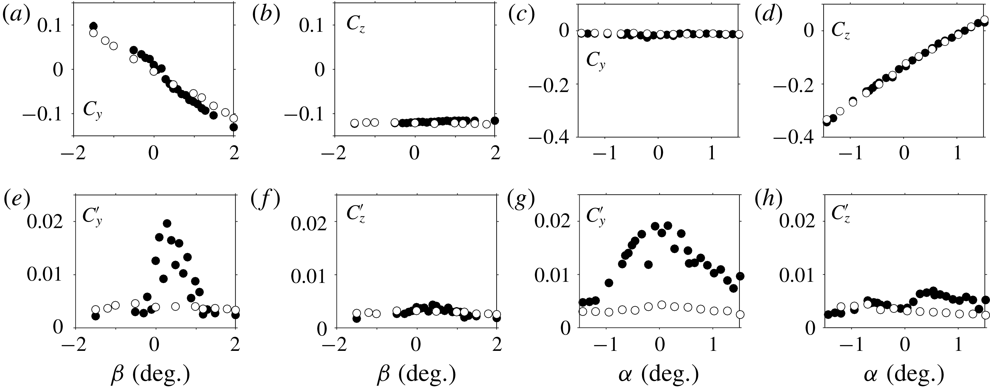
Figure 11. Mean (a–d) and fluctuating (e–h) cross-flow force coefficients versus yaw (a,b,e,f) and pitch angle (c,d,g,h) of the square-back body (black filled circles) and with the rear cavity (empty circles).

Figure 12. Mean side force coefficient versus yaw
 $\unicode[STIX]{x1D6FD}$
of the square-back body. In (a), measured force coefficient (symbols), basic flow coefficient (red line) and coefficient computed from (3.1) (blue dashed line, see text). In (b), mean contribution of the instability
$\unicode[STIX]{x1D6FD}$
of the square-back body. In (a), measured force coefficient (symbols), basic flow coefficient (red line) and coefficient computed from (3.1) (blue dashed line, see text). In (b), mean contribution of the instability
 $C_{y}-C_{y}^{B}$
(filled circles) and mean horizontal base pressure gradient
$C_{y}-C_{y}^{B}$
(filled circles) and mean horizontal base pressure gradient
 $G_{y}^{\ast }$
(crosses).
$G_{y}^{\ast }$
(crosses).

Figure 13. Components of the fluctuation force coefficients of the square-back body
 $C_{y}^{\prime }$
and
$C_{y}^{\prime }$
and
 $C_{z}^{\prime }$
(filled circles) compared to the fluctuation base pressure gradient
$C_{z}^{\prime }$
(filled circles) compared to the fluctuation base pressure gradient
 ${G_{y}^{\ast }}^{\prime }$
and
${G_{y}^{\ast }}^{\prime }$
and
 ${G_{z}^{\ast }}^{\prime }$
(crosses) versus yaw
${G_{z}^{\ast }}^{\prime }$
(crosses) versus yaw
 $\unicode[STIX]{x1D6FD}$
(a,c) and pitch angle
$\unicode[STIX]{x1D6FD}$
(a,c) and pitch angle
 $\unicode[STIX]{x1D6FC}$
(b,d).
$\unicode[STIX]{x1D6FC}$
(b,d).
3.1.3 Global force sensitivity versus wake aerodynamic loading
The
 $y$
- and
$y$
- and
 $z$
-components of the mean force coefficients obtained for the yaw and pitch sensitivity experiments are shown in figure 11(a–d) with and without the rear cavity. A clear stabilization of the unstable wake can be seen in the mean horizontal
$z$
-components of the mean force coefficients obtained for the yaw and pitch sensitivity experiments are shown in figure 11(a–d) with and without the rear cavity. A clear stabilization of the unstable wake can be seen in the mean horizontal
 $y$
-component in figure 11(a) obtained with the yaw variations. The nonlinear behaviour due to the instability (also reported in Perry et al. (Reference Perry, Pavia and Passmore2016b
)) is replaced by a linear law with the cavity. For the other mean coefficients, we can hardly distinguish any effect induced by the rear cavity. For the force coefficient fluctuations shown in figure 11(e–h), one can observe fluctuation crisis each time phase unlocking occurs.
$y$
-component in figure 11(a) obtained with the yaw variations. The nonlinear behaviour due to the instability (also reported in Perry et al. (Reference Perry, Pavia and Passmore2016b
)) is replaced by a linear law with the cavity. For the other mean coefficients, we can hardly distinguish any effect induced by the rear cavity. For the force coefficient fluctuations shown in figure 11(e–h), one can observe fluctuation crisis each time phase unlocking occurs.
Figure 11(a) suggests that the mean side force coefficient
 $C_{y}^{B}$
obtained without the instability (the superscript
$C_{y}^{B}$
obtained without the instability (the superscript
 $^{B}$
will refer to this basic flow) should evolve linearly with
$^{B}$
will refer to this basic flow) should evolve linearly with
 $\unicode[STIX]{x1D6FD}$
as for the cavity experiment. The force coefficient
$\unicode[STIX]{x1D6FD}$
as for the cavity experiment. The force coefficient
 $C_{y}^{B}(\unicode[STIX]{x1D6FD})=-0.055\times \unicode[STIX]{x1D6FD}$
(where
$C_{y}^{B}(\unicode[STIX]{x1D6FD})=-0.055\times \unicode[STIX]{x1D6FD}$
(where
 $\unicode[STIX]{x1D6FD}$
is expressed in degrees), simply obtained from a linear fit of the cavity experiment, is shown in figure 12(a) as the red straight line. We compare the strength of the instability
$\unicode[STIX]{x1D6FD}$
is expressed in degrees), simply obtained from a linear fit of the cavity experiment, is shown in figure 12(a) as the red straight line. We compare the strength of the instability
 $C_{y}-C_{y}^{B}$
to the mean horizontal base pressure gradient
$C_{y}-C_{y}^{B}$
to the mean horizontal base pressure gradient
 $G_{y}^{\ast }$
in figure 12(b). The two curves are satisfactorily proportional such that the mean side force coefficient can be directly related to the mean base gradient as:
$G_{y}^{\ast }$
in figure 12(b). The two curves are satisfactorily proportional such that the mean side force coefficient can be directly related to the mean base gradient as:
 $$\begin{eqnarray}\displaystyle C_{y}=C_{y}^{B}-\frac{G_{y}^{\ast }}{10}. & & \displaystyle\end{eqnarray}$$
We can see in figure 12(a) the good agreement of (3.1) (blue dashed line) with the experimental data (symbols). An instantaneous relationship can be speculated from (3.1) to take into account the unsteady loading due to the wake instability through the dynamics of the base gradient:
 $$\begin{eqnarray}\displaystyle c_{y}(t^{\ast })=C_{y}^{B}-\frac{g_{y}^{\ast }(t^{\ast })}{10} & & \displaystyle\end{eqnarray}$$
implying that
 $C_{y}^{\prime }={G_{y}^{\ast }}^{\prime }/10$
. The fluctuation force coefficient
$C_{y}^{\prime }={G_{y}^{\ast }}^{\prime }/10$
. The fluctuation force coefficient
 $C_{y}^{\prime }$
is plotted in figure 13(a) for yaw variation and figure 13(b) for pitch variation and matches satisfactorily with
$C_{y}^{\prime }$
is plotted in figure 13(a) for yaw variation and figure 13(b) for pitch variation and matches satisfactorily with
 ${G^{\ast }}_{y}^{\prime }/10$
.
${G^{\ast }}_{y}^{\prime }/10$
.
Since the mean lift coefficient
 $C_{z}$
is not affected by the instability (no differences in figure 11(b,d) with or without the rear cavity), we can state that for the vertical force coefficient:
$C_{z}$
is not affected by the instability (no differences in figure 11(b,d) with or without the rear cavity), we can state that for the vertical force coefficient:
 $$\begin{eqnarray}\displaystyle C_{z}=C_{z}^{B} & & \displaystyle\end{eqnarray}$$
regardless of the base pressure gradient orientation. Again, an instantaneous relationship but with only the fluctuations of the vertical gradient component can be speculated:
 $$\begin{eqnarray}\displaystyle c_{z}(t^{\ast })=C_{z}^{B}-\frac{{g^{\ast }}_{z}^{\prime }(t^{\ast })}{10} & & \displaystyle\end{eqnarray}$$
implying that
 ${C_{z}}^{\prime }={G_{z}^{\ast }}^{\prime }/10$
. Although the fluctuations are much smaller vertically than horizontally, we still see good agreements of (3.4) in figure 13(c,d).
${C_{z}}^{\prime }={G_{z}^{\ast }}^{\prime }/10$
. Although the fluctuations are much smaller vertically than horizontally, we still see good agreements of (3.4) in figure 13(c,d).
One may wonder if a similar relationship could be obtained from the drag
 $c_{x}$
and the base suction
$c_{x}$
and the base suction
 $c_{b}$
coefficients. Actually, independently of the ground clearance, the yaw or the pitch, the rear cavity has a beneficial effect on the mean base suction or mean drag coefficient that are respectively reduced within the ranges
$c_{b}$
coefficients. Actually, independently of the ground clearance, the yaw or the pitch, the rear cavity has a beneficial effect on the mean base suction or mean drag coefficient that are respectively reduced within the ranges
 $[23\,\%,25\,\%]$
and
$[23\,\%,25\,\%]$
and
 $[9.5\,\%,10.5\,\%]$
as can be seen in figure 14(a–d). Comparable drag reduction is also observed below the instability threshold (
$[9.5\,\%,10.5\,\%]$
as can be seen in figure 14(a–d). Comparable drag reduction is also observed below the instability threshold (
 $c^{\ast }<0.105$
). As shown in Lucas et al. (Reference Lucas, Cadot, Herbert, Parpais and Délery2017), a deep rear cavity has a primary effect of considerably lengthening the recirculating region towards the inside of the body. Consequently, low pressure sources therein are reduced independently from the symmetry properties of the wake. It then remains impossible to distinguish the contribution from the wake symmetrization due to the instability suppression to this strong mean flow modification. Hence, from our point of view, the drag of the basic flow
$c^{\ast }<0.105$
). As shown in Lucas et al. (Reference Lucas, Cadot, Herbert, Parpais and Délery2017), a deep rear cavity has a primary effect of considerably lengthening the recirculating region towards the inside of the body. Consequently, low pressure sources therein are reduced independently from the symmetry properties of the wake. It then remains impossible to distinguish the contribution from the wake symmetrization due to the instability suppression to this strong mean flow modification. Hence, from our point of view, the drag of the basic flow
 $C_{x}^{B}$
is not extractable from the data. Considering all yaw and pitch variations, the fluctuations of both the base suction and drag remain almost identical to those of the baseline given in table 2 as can be seen in figure 14(e–h). There are then no consequences of the unstable wake phase dynamics on these coefficients. The reason is that base suction is more related to the magnitude of the gradient’s modulus that was shown to be almost constant rather than to its orientation. The correlation between base suction and the gradient’s modulus was previously reported in the sensitivity analysis to a disturbance placed in the wake by Grandemange et al. (Reference Grandemange, Gohlke and Cadot2014b
) or instantaneously by Evrard et al. (Reference Evrard, Cadot, Herbert, Ricot, Vigneron and Délery2016).
$C_{x}^{B}$
is not extractable from the data. Considering all yaw and pitch variations, the fluctuations of both the base suction and drag remain almost identical to those of the baseline given in table 2 as can be seen in figure 14(e–h). There are then no consequences of the unstable wake phase dynamics on these coefficients. The reason is that base suction is more related to the magnitude of the gradient’s modulus that was shown to be almost constant rather than to its orientation. The correlation between base suction and the gradient’s modulus was previously reported in the sensitivity analysis to a disturbance placed in the wake by Grandemange et al. (Reference Grandemange, Gohlke and Cadot2014b
) or instantaneously by Evrard et al. (Reference Evrard, Cadot, Herbert, Ricot, Vigneron and Délery2016).

Figure 14. Mean (a–d) and fluctuating (e–h) drag force and base suction coefficients versus yaw (a,b,e,f) and pitch angle (c,d,g,h) of the square-back body (black filled circles) and with the rear cavity (empty circles).
3.2 The
$z$
-instability

This section presents the results about the boat-tailed geometry depicted in figure 2(d) and with a base aspect ratio of
 $w_{b}^{\ast }=0.940$
. In § 3.2.1, we show sensitivity maps of the base pressure gradient responses to variations of the ground clearance
$w_{b}^{\ast }=0.940$
. In § 3.2.1, we show sensitivity maps of the base pressure gradient responses to variations of the ground clearance
 $c^{\ast }$
, the yaw angle
$c^{\ast }$
, the yaw angle
 $\unicode[STIX]{x1D6FD}$
and the pitch angle
$\unicode[STIX]{x1D6FD}$
and the pitch angle
 $\unicode[STIX]{x1D6FC}$
around the baseline exactly as in § 3.1.1. The wake topologies and dynamics are then investigated for chosen specific configurations reflecting all situations. The yaw sensitivities are repeated in § 3.2.2 for different ground clearances to evidence the two branches of most probable states of the wake. The aerodynamic force is examined in a third part § 3.2.3.
$\unicode[STIX]{x1D6FC}$
around the baseline exactly as in § 3.1.1. The wake topologies and dynamics are then investigated for chosen specific configurations reflecting all situations. The yaw sensitivities are repeated in § 3.2.2 for different ground clearances to evidence the two branches of most probable states of the wake. The aerodynamic force is examined in a third part § 3.2.3.
3.2.1 Wake sensitivity to the body clearance and orientations
The four sensitivity maps of the base pressure gradient due to the variation of the ground clearance
 $c^{\ast }$
are shown in figure 15(a,b) for the Cartesian components and figure 15(c,d) for the polar form. When the ground clearance is gradually increased in figure 15(a), the horizontal component
$c^{\ast }$
are shown in figure 15(a,b) for the Cartesian components and figure 15(c,d) for the polar form. When the ground clearance is gradually increased in figure 15(a), the horizontal component
 $g_{y}^{\ast }$
remains almost around zero. The vertical component
$g_{y}^{\ast }$
remains almost around zero. The vertical component
 $g_{z}^{\ast }$
(figure 15
b) experiences a jump for
$g_{z}^{\ast }$
(figure 15
b) experiences a jump for
 $c^{\ast }\simeq 0.080$
from a positive branch (
$c^{\ast }\simeq 0.080$
from a positive branch (
 $g_{z}^{\ast }\simeq 0.1$
) to a negative one (
$g_{z}^{\ast }\simeq 0.1$
) to a negative one (
 $g_{z}^{\ast }\simeq -0.1$
). A bistable dynamics is then obtained around
$g_{z}^{\ast }\simeq -0.1$
). A bistable dynamics is then obtained around
 $c^{\ast }\simeq 0.080$
. In the experiment of Grandemange et al. (Reference Grandemange, Gohlke and Cadot2013a
), the ground clearance is non-dimensionalized using the body width,
$c^{\ast }\simeq 0.080$
. In the experiment of Grandemange et al. (Reference Grandemange, Gohlke and Cadot2013a
), the ground clearance is non-dimensionalized using the body width,
 $c_{W}^{\ast }=c^{\ast }/W^{\ast }$
, and the
$c_{W}^{\ast }=c^{\ast }/W^{\ast }$
, and the
 $z$
-instability is found to saturate on the positive branch only for a ground clearance
$z$
-instability is found to saturate on the positive branch only for a ground clearance
 $c_{SW}^{\ast }\simeq 0.060$
and then switches to the negative branch at
$c_{SW}^{\ast }\simeq 0.060$
and then switches to the negative branch at
 $c_{W}^{\ast }\simeq 0.1$
. Our experiment satisfactorily reproduces the switch from the positive to the negative branch but with smaller ground clearance. Using non-dimensionalization of Grandemange et al. (Reference Grandemange, Gohlke and Cadot2013a
), the switch we observe at
$c_{W}^{\ast }\simeq 0.1$
. Our experiment satisfactorily reproduces the switch from the positive to the negative branch but with smaller ground clearance. Using non-dimensionalization of Grandemange et al. (Reference Grandemange, Gohlke and Cadot2013a
), the switch we observe at
 $c^{\ast }\simeq 0.080$
in figure 15 is within the range
$c^{\ast }\simeq 0.080$
in figure 15 is within the range
 $0.068\lesssim c_{W}^{\ast }\lesssim 0.085$
when translated using either
$0.068\lesssim c_{W}^{\ast }\lesssim 0.085$
when translated using either
 $W^{\ast }$
or
$W^{\ast }$
or
 $w_{b}^{\ast }$
of the boat-tailed body. The range remains below the value
$w_{b}^{\ast }$
of the boat-tailed body. The range remains below the value
 $c_{W}^{\ast }\simeq 0.1$
of Grandemange et al. (Reference Grandemange, Gohlke and Cadot2013a
). This can be ascribed to a Reynolds number effect, which is approximately ten times larger in the present study (
$c_{W}^{\ast }\simeq 0.1$
of Grandemange et al. (Reference Grandemange, Gohlke and Cadot2013a
). This can be ascribed to a Reynolds number effect, which is approximately ten times larger in the present study (
 $Re\simeq 4.0\times 10^{5}$
) than in Grandemange et al. (Reference Grandemange, Gohlke and Cadot2013a
) (
$Re\simeq 4.0\times 10^{5}$
) than in Grandemange et al. (Reference Grandemange, Gohlke and Cadot2013a
) (
 $Re\simeq 4.5\times 10^{4}$
). It is in accordance with Reynolds number effect studied in Cadot et al. (Reference Cadot, Evrard and Pastur2015) who report a
$Re\simeq 4.5\times 10^{4}$
). It is in accordance with Reynolds number effect studied in Cadot et al. (Reference Cadot, Evrard and Pastur2015) who report a
 $30\,\%$
decrease of the critical ground clearance for the
$30\,\%$
decrease of the critical ground clearance for the
 $y$
-instability when the Reynolds number is increased from
$y$
-instability when the Reynolds number is increased from
 $1.7\times 10^{4}$
to
$1.7\times 10^{4}$
to
 $1.6\times 10^{5}$
. The critical ground clearance
$1.6\times 10^{5}$
. The critical ground clearance
 $c_{S}^{\ast }$
of the
$c_{S}^{\ast }$
of the
 $z$
-instability is not observed in our study because it is below the minimal value
$z$
-instability is not observed in our study because it is below the minimal value
 $c^{\ast }=0.05$
allowed by the set-up. It is also found that the critical ground clearance is larger for the
$c^{\ast }=0.05$
allowed by the set-up. It is also found that the critical ground clearance is larger for the
 $y$
-instability than for the
$y$
-instability than for the
 $z$
-instability as in Grandemange et al. (Reference Grandemange, Gohlke and Cadot2013a
). The modulus
$z$
-instability as in Grandemange et al. (Reference Grandemange, Gohlke and Cadot2013a
). The modulus
 $g_{r}^{\ast }$
displayed in figure 15(c) has a value close to
$g_{r}^{\ast }$
displayed in figure 15(c) has a value close to
 $0.1$
that is smaller than the modulus found within the range
$0.1$
that is smaller than the modulus found within the range
 $0.15{-}0.2$
(see figures 3
c, 4
c, 5
c) in § 3.1 for the square-back body. This must be ascribed to the different after-body geometry. The larger fluctuations observed for
$0.15{-}0.2$
(see figures 3
c, 4
c, 5
c) in § 3.1 for the square-back body. This must be ascribed to the different after-body geometry. The larger fluctuations observed for
 $c^{\ast }\simeq 0.080$
are a consequence of the bistable dynamics at the branches switch in figure 15(d).
$c^{\ast }\simeq 0.080$
are a consequence of the bistable dynamics at the branches switch in figure 15(d).

Figure 15. Base pressure gradient response to a variation of the ground clearance
 $c^{\ast }$
for the boat-tailed body. Sensitivity maps (a)
$c^{\ast }$
for the boat-tailed body. Sensitivity maps (a)
 $f(c^{\ast },g_{y}^{\ast })$
, (b)
$f(c^{\ast },g_{y}^{\ast })$
, (b)
 $f(c^{\ast },g_{z}^{\ast })$
, (c)
$f(c^{\ast },g_{z}^{\ast })$
, (c)
 $f(c^{\ast },g_{r}^{\ast })$
and (d)
$f(c^{\ast },g_{r}^{\ast })$
and (d)
 $f(c^{\ast },\unicode[STIX]{x1D711})$
.
$f(c^{\ast },\unicode[STIX]{x1D711})$
.
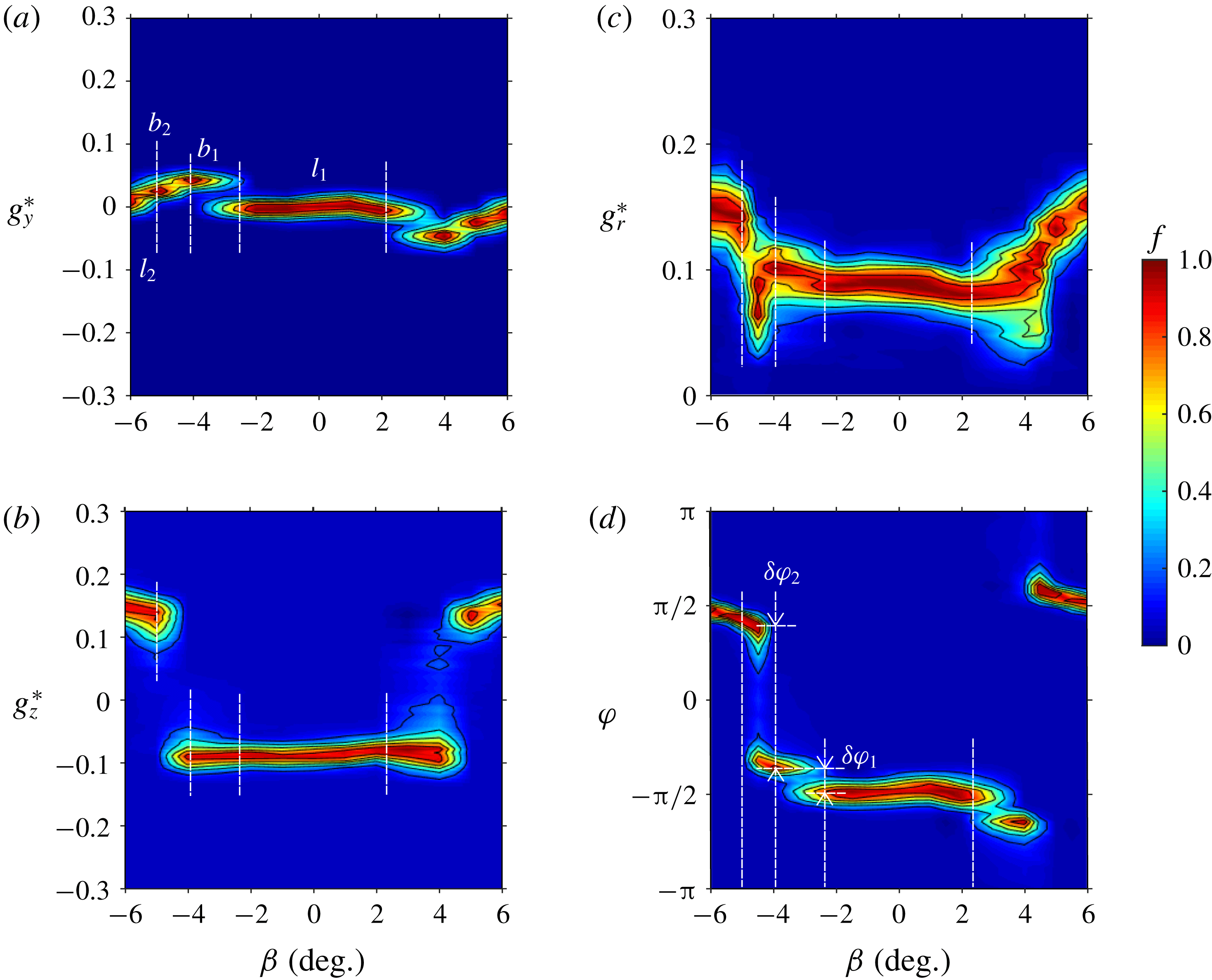
Figure 16. Base pressure gradient response to variations of the yaw angle
 $\unicode[STIX]{x1D6FD}$
for the boat-tailed body. Sensitivity maps (a)
$\unicode[STIX]{x1D6FD}$
for the boat-tailed body. Sensitivity maps (a)
 $f(\unicode[STIX]{x1D6FD},g_{y}^{\ast })$
, (b)
$f(\unicode[STIX]{x1D6FD},g_{y}^{\ast })$
, (b)
 $f(\unicode[STIX]{x1D6FD},g_{z}^{\ast })$
, (c)
$f(\unicode[STIX]{x1D6FD},g_{z}^{\ast })$
, (c)
 $f(\unicode[STIX]{x1D6FD},g_{r}^{\ast })$
and (d)
$f(\unicode[STIX]{x1D6FD},g_{r}^{\ast })$
and (d)
 $f(\unicode[STIX]{x1D6FD},\unicode[STIX]{x1D711})$
.
$f(\unicode[STIX]{x1D6FD},\unicode[STIX]{x1D711})$
.
Figure 17. Base pressure gradient response to variations of the pitch angle
 $\unicode[STIX]{x1D6FC}$
for the boat-tailed body. Sensitivity maps (a)
$\unicode[STIX]{x1D6FC}$
for the boat-tailed body. Sensitivity maps (a)
 $f(\unicode[STIX]{x1D6FC},g_{y}^{\ast })$
, (b)
$f(\unicode[STIX]{x1D6FC},g_{y}^{\ast })$
, (b)
 $f(\unicode[STIX]{x1D6FC},g_{z}^{\ast })$
, (c)
$f(\unicode[STIX]{x1D6FC},g_{z}^{\ast })$
, (c)
 $f(\unicode[STIX]{x1D6FC},g_{r}^{\ast })$
and (d)
$f(\unicode[STIX]{x1D6FC},g_{r}^{\ast })$
and (d)
 $f(\unicode[STIX]{x1D6FC},\unicode[STIX]{x1D711})$
.
$f(\unicode[STIX]{x1D6FC},\unicode[STIX]{x1D711})$
.

Figure 18. Modulus
 $g_{r\unicode[STIX]{x1D6FC}}^{\ast }(t^{\ast })$
and phase
$g_{r\unicode[STIX]{x1D6FC}}^{\ast }(t^{\ast })$
and phase
 $\unicode[STIX]{x1D711}_{\unicode[STIX]{x1D6FC}}(t^{\ast })$
time series (left) of the base pressure gradient for the boat-tailed body. Corresponding probability density functions (right) for (a)
$\unicode[STIX]{x1D711}_{\unicode[STIX]{x1D6FC}}(t^{\ast })$
time series (left) of the base pressure gradient for the boat-tailed body. Corresponding probability density functions (right) for (a)
 $\unicode[STIX]{x1D6FD}=-3^{\circ }$
, (b)
$\unicode[STIX]{x1D6FD}=-3^{\circ }$
, (b)
 $\unicode[STIX]{x1D6FD}=-5^{\circ }$
. The smooth red lines superimposed on the PDFs (
$\unicode[STIX]{x1D6FD}=-5^{\circ }$
. The smooth red lines superimposed on the PDFs (
 $g_{r}^{\ast }$
) in (a) and (b) are best fits of Rigas et al.’s (Reference Rigas, Morgans, Brackston and Morrison2015) PDF model; the three parameters of the fit are not given.
$g_{r}^{\ast }$
) in (a) and (b) are best fits of Rigas et al.’s (Reference Rigas, Morgans, Brackston and Morrison2015) PDF model; the three parameters of the fit are not given.

Figure 19. Cross-sections of the mean velocity field for the boat-tailed body visualized using streamlines superimposed on the modulus of the components in the vertical plane
 $(x^{\ast },z^{\ast })$
for (a) baseline configuration (
$(x^{\ast },z^{\ast })$
for (a) baseline configuration (
 $\unicode[STIX]{x1D6FC}=\unicode[STIX]{x1D6FD}=0^{\circ }$
,
$\unicode[STIX]{x1D6FC}=\unicode[STIX]{x1D6FD}=0^{\circ }$
,
 $c^{\ast }=0.168$
), (b)
$c^{\ast }=0.168$
), (b)
 $\unicode[STIX]{x1D6FC}=\unicode[STIX]{x1D6FD}=0^{\circ }$
,
$\unicode[STIX]{x1D6FC}=\unicode[STIX]{x1D6FD}=0^{\circ }$
,
 $c^{\ast }=0.060$
, (c)
$c^{\ast }=0.060$
, (c)
 $\unicode[STIX]{x1D6FC}=0^{\circ }$
,
$\unicode[STIX]{x1D6FC}=0^{\circ }$
,
 $\unicode[STIX]{x1D6FD}=-5^{\circ }$
,
$\unicode[STIX]{x1D6FD}=-5^{\circ }$
,
 $c^{\ast }=0.168$
, (d) nose-down configuration
$c^{\ast }=0.168$
, (d) nose-down configuration
 $\unicode[STIX]{x1D6FC}=-0.6^{\circ }$
(
$\unicode[STIX]{x1D6FC}=-0.6^{\circ }$
(
 $\unicode[STIX]{x1D6FD}=0^{\circ }$
). The associated mean base pressure distributions
$\unicode[STIX]{x1D6FD}=0^{\circ }$
). The associated mean base pressure distributions
 $C_{p}(y^{\ast },z^{\ast })$
are also provided.
$C_{p}(y^{\ast },z^{\ast })$
are also provided.
For the next two series of experiments concerning yaw and pitch sensitivities, we will consider small variations of the inclination around the baseline with characteristics given in table 2.
The sensitivity analysis to the yaw angle
 $\unicode[STIX]{x1D6FD}$
with a fixed pitch
$\unicode[STIX]{x1D6FD}$
with a fixed pitch
 $\unicode[STIX]{x1D6FC}=0^{\circ }$
is shown in figure 16. The results being reasonably symmetric with respect to
$\unicode[STIX]{x1D6FC}=0^{\circ }$
is shown in figure 16. The results being reasonably symmetric with respect to
 $\unicode[STIX]{x1D6FD}$
, we only comment the part for
$\unicode[STIX]{x1D6FD}$
, we only comment the part for
 $\unicode[STIX]{x1D6FD}<0^{\circ }$
. From these figures, four distinctive regions can be observed, successively named
$\unicode[STIX]{x1D6FD}<0^{\circ }$
. From these figures, four distinctive regions can be observed, successively named
 $l_{1}$
,
$l_{1}$
,
 $b_{1}$
,
$b_{1}$
,
 $b_{2}$
and
$b_{2}$
and
 $l_{2}$
in figure 16(a). They are delimited in all the figures by vertical dashed lines. In region
$l_{2}$
in figure 16(a). They are delimited in all the figures by vertical dashed lines. In region
 $l_{1}$
the base pressure gradient remains almost identical to that of the baseline: it is locked with a vertical direction orientated towards the ground corresponding to
$l_{1}$
the base pressure gradient remains almost identical to that of the baseline: it is locked with a vertical direction orientated towards the ground corresponding to
 $\unicode[STIX]{x1D711}\simeq -\unicode[STIX]{x03C0}/2$
in figure 16(d) and a modulus close to
$\unicode[STIX]{x1D711}\simeq -\unicode[STIX]{x03C0}/2$
in figure 16(d) and a modulus close to
 $g_{r}^{\ast }\simeq 0.1$
in figure 16(c). When the yaw angle
$g_{r}^{\ast }\simeq 0.1$
in figure 16(c). When the yaw angle
 $\unicode[STIX]{x1D6FD}$
is increased, the wake becomes bistable in the region
$\unicode[STIX]{x1D6FD}$
is increased, the wake becomes bistable in the region
 $b_{1}$
and the gradient experiences small phase jumps of amplitude
$b_{1}$
and the gradient experiences small phase jumps of amplitude
 $\unicode[STIX]{x1D6FF}\unicode[STIX]{x1D711}_{1}\simeq \unicode[STIX]{x03C0}/7$
without noticeable changes in the modulus
$\unicode[STIX]{x1D6FF}\unicode[STIX]{x1D711}_{1}\simeq \unicode[STIX]{x03C0}/7$
without noticeable changes in the modulus
 $g_{r}^{\ast }$
. This small lateral bistability has not been observed for yaw experiments at lower ground clearance – for which transitions occur at smaller angles – presented in § 3.2.2. Although not discernible on the side pressure measurements, it is suspected to be caused by premises of separation on the leeward boat tail. For larger yaw angles, another bistable regime in
$g_{r}^{\ast }$
. This small lateral bistability has not been observed for yaw experiments at lower ground clearance – for which transitions occur at smaller angles – presented in § 3.2.2. Although not discernible on the side pressure measurements, it is suspected to be caused by premises of separation on the leeward boat tail. For larger yaw angles, another bistable regime in
 $b_{2}$
is observed with much larger phase jumps of
$b_{2}$
is observed with much larger phase jumps of
 $\unicode[STIX]{x1D6FF}\unicode[STIX]{x1D711}_{2}\simeq 3\unicode[STIX]{x03C0}/4$
in figure 16(d) associated with large fluctuations of the modulus. In the last regime
$\unicode[STIX]{x1D6FF}\unicode[STIX]{x1D711}_{2}\simeq 3\unicode[STIX]{x03C0}/4$
in figure 16(d) associated with large fluctuations of the modulus. In the last regime
 $l_{2}$
, the gradient is locked with a vertical direction orientated towards the top (
$l_{2}$
, the gradient is locked with a vertical direction orientated towards the top (
 $\unicode[STIX]{x1D711}\simeq +\unicode[STIX]{x03C0}/2$
) and a modulus close to
$\unicode[STIX]{x1D711}\simeq +\unicode[STIX]{x03C0}/2$
) and a modulus close to
 $g_{r}^{\ast }\simeq 0.15$
. The main result is that the yaw around
$g_{r}^{\ast }\simeq 0.15$
. The main result is that the yaw around
 $\unicode[STIX]{x1D6FD}=\pm 4.5^{\circ }$
triggers the switch of the negative vertical pressure gradient component of the baseline observed in
$\unicode[STIX]{x1D6FD}=\pm 4.5^{\circ }$
triggers the switch of the negative vertical pressure gradient component of the baseline observed in
 $l_{1}$
to a positive vertical component in
$l_{1}$
to a positive vertical component in
 $l_{2}$
as clearly shown in figure 16(b).
$l_{2}$
as clearly shown in figure 16(b).
The sensitivity towards the pitch angle
 $\unicode[STIX]{x1D6FC}$
is now given in figure 17. For this experiment, the yaw angle is set to
$\unicode[STIX]{x1D6FC}$
is now given in figure 17. For this experiment, the yaw angle is set to
 $\unicode[STIX]{x1D6FD}=0^{\circ }$
and, as in § 3.1, the front and rear ground clearances are adjusted for a given pitch but keeping
$\unicode[STIX]{x1D6FD}=0^{\circ }$
and, as in § 3.1, the front and rear ground clearances are adjusted for a given pitch but keeping
 $c^{\ast }=(c_{f}^{\ast }+c_{r}^{\ast })/2=0.168$
. Based on the mechanism identified for the
$c^{\ast }=(c_{f}^{\ast }+c_{r}^{\ast })/2=0.168$
. Based on the mechanism identified for the
 $y$
-instability in § 3.1, we restricted the range of pitch angles to nose-down configurations for which a clear transition is observed. The pitch angle has almost no effect on the horizontal component in figure 17(a) except for a disturbance around
$y$
-instability in § 3.1, we restricted the range of pitch angles to nose-down configurations for which a clear transition is observed. The pitch angle has almost no effect on the horizontal component in figure 17(a) except for a disturbance around
 $\unicode[STIX]{x1D6FC}=-0.4^{\circ }$
that corresponds to the switching region with a bistable dynamics in figure 17(b) of the vertical component of the gradient.
$\unicode[STIX]{x1D6FC}=-0.4^{\circ }$
that corresponds to the switching region with a bistable dynamics in figure 17(b) of the vertical component of the gradient.
The successive experiments changing ground clearance, pitch and yaw mainly show that for the boat-tailed body subjected to the
 $z$
-instability, two principal orientations of the base pressure gradient are observed: almost positive vertical and negative vertical. The phase then remains locked except for the bistable dynamics where the wake switches between opposite orientations. The dynamics of the two bistable cases
$z$
-instability, two principal orientations of the base pressure gradient are observed: almost positive vertical and negative vertical. The phase then remains locked except for the bistable dynamics where the wake switches between opposite orientations. The dynamics of the two bistable cases
 $b_{1}$
and
$b_{1}$
and
 $b_{2}$
evidenced during the yaw sensitivity in figure 16(c) is respectively presented in figure 18(a) and figure 18(b). The bistable dynamics
$b_{2}$
evidenced during the yaw sensitivity in figure 16(c) is respectively presented in figure 18(a) and figure 18(b). The bistable dynamics
 $b_{2}$
is similar to that obtained in ground clearance sensitivity (figure 15
c) and pitch sensitivity (figure 17
c) analyses. The striking observation is that the rate of random switching between the two most probable phases is substantially larger than that of the bistable wake subjected to the
$b_{2}$
is similar to that obtained in ground clearance sensitivity (figure 15
c) and pitch sensitivity (figure 17
c) analyses. The striking observation is that the rate of random switching between the two most probable phases is substantially larger than that of the bistable wake subjected to the
 $y$
-instability in figure 6(b). For the most important bistable behaviour that involves vertical wake reversals in figure 18(b), approximately
$y$
-instability in figure 6(b). For the most important bistable behaviour that involves vertical wake reversals in figure 18(b), approximately
 $50$
switches are observed against only
$50$
switches are observed against only
 $9$
in figure 6(b) for horizontal wake reversals. This trend was checked for all bistable cases, thus confirming that the characteristic time of the random switching is approximately five times smaller for the
$9$
in figure 6(b) for horizontal wake reversals. This trend was checked for all bistable cases, thus confirming that the characteristic time of the random switching is approximately five times smaller for the
 $z$
-instability than for the
$z$
-instability than for the
 $y$
-instability.
$y$
-instability.
The different wake configurations are illustrated by their mean flow in the vertical plane in figure 19 together with their corresponding mean base pressure distribution. Because of the boat tailing, the after-body develops four strong longitudinal vortices at each corner of the base affecting considerably the mean bubble closure in the figure 19 compared to that observed for the square-back after-body in figures 7 and 10. For the baseline in figure 19(a), the negative vertical pressure gradient observed in the pressure distribution is associated with a skewed feedback flow orientated towards the bottom edge of the base that is the best topological indicator of the
 $z$
-instability. We have identified wake reversals from the baseline for each of the three sensitivity experiments either by decreasing the ground clearance, increasing the yaw angle or by pitching down the body. For a lower ground clearance, the wake has effectively switched to the opposite base pressure gradient in figure 19(b) with a skewed feedback flow orientated to the top edge of the base. For a large yaw in figure 19(c), the switch from the baseline is not clearly observable in the vertical velocity field, while it is clearly established in the corresponding pressure distribution. Finally, for large nose-down pitch, the skewed feedback flow and the pressure distribution are clearly inverted from those of the baseline.
$z$
-instability. We have identified wake reversals from the baseline for each of the three sensitivity experiments either by decreasing the ground clearance, increasing the yaw angle or by pitching down the body. For a lower ground clearance, the wake has effectively switched to the opposite base pressure gradient in figure 19(b) with a skewed feedback flow orientated to the top edge of the base. For a large yaw in figure 19(c), the switch from the baseline is not clearly observable in the vertical velocity field, while it is clearly established in the corresponding pressure distribution. Finally, for large nose-down pitch, the skewed feedback flow and the pressure distribution are clearly inverted from those of the baseline.
3.2.2 Exploration of the most probable states
We now investigate the wake reversals with yaw for different fixed ground clearances:
 $c^{\ast }=0.060$
;
$c^{\ast }=0.060$
;
 $0.080$
;
$0.080$
;
 $0.124$
;
$0.124$
;
 $0.168$
and a pitch angle set at
$0.168$
and a pitch angle set at
 $\unicode[STIX]{x1D6FC}=0^{\circ }$
. With no yaw angle, we can see from figure 15(a,b) that these ground clearances successively correspond to a locked positive vertical gradient for
$\unicode[STIX]{x1D6FC}=0^{\circ }$
. With no yaw angle, we can see from figure 15(a,b) that these ground clearances successively correspond to a locked positive vertical gradient for
 $c^{\ast }=0.060$
, a bistable dynamics for
$c^{\ast }=0.060$
, a bistable dynamics for
 $c^{\ast }=0.080$
and a locked negative vertical gradient for
$c^{\ast }=0.080$
and a locked negative vertical gradient for
 $c^{\ast }=0.124$
and
$c^{\ast }=0.124$
and
 $c^{\ast }=0.168$
. It is remarkable that the ground clearance has almost no effect on the gradient modulus in figure 15(c). So, it seems that the ground orientates the unstable wake with a positive vertical gradient for small
$c^{\ast }=0.168$
. It is remarkable that the ground clearance has almost no effect on the gradient modulus in figure 15(c). So, it seems that the ground orientates the unstable wake with a positive vertical gradient for small
 $c^{\ast }$
and with a negative vertical gradient for large
$c^{\ast }$
and with a negative vertical gradient for large
 $c^{\ast }$
. At large ground clearance we would have expected the ground to become irrelevant and that the recovery of the top/down symmetry of the flow would have led to a bistable dynamics independently of the ground proximity. It is then the presence of the four supports that is responsible for the locked wake orientation at large ground clearance.
$c^{\ast }$
. At large ground clearance we would have expected the ground to become irrelevant and that the recovery of the top/down symmetry of the flow would have led to a bistable dynamics independently of the ground proximity. It is then the presence of the four supports that is responsible for the locked wake orientation at large ground clearance.

Figure 20. Most probable pressure gradients for the boat-tailed body
 $g_{y}^{\ast }$
and
$g_{y}^{\ast }$
and
 $g_{z}^{\ast }$
(a),
$g_{z}^{\ast }$
(a),
 $g_{r}^{\ast }$
(b) and
$g_{r}^{\ast }$
(b) and
 $\unicode[STIX]{x1D711}$
(c) versus the yaw angle at different ground clearances (with descending values from top to bottom in a). The triangles at
$\unicode[STIX]{x1D711}$
(c) versus the yaw angle at different ground clearances (with descending values from top to bottom in a). The triangles at
 $\unicode[STIX]{x1D6FD}=0^{\circ }$
correspond to the experiment with a fifth cylindrical support (see text).
$\unicode[STIX]{x1D6FD}=0^{\circ }$
correspond to the experiment with a fifth cylindrical support (see text).
Sensitivity analyses with the yaw angle limited to
 $\unicode[STIX]{x1D6FD}\in [-6^{\circ },0^{\circ }]$
are presented in figure 20. For clarity, we extract the branches of most probable gradients using the following technique. The location of the maxima of each branch of the sensitivity maps such as the one given in figure 16 for
$\unicode[STIX]{x1D6FD}\in [-6^{\circ },0^{\circ }]$
are presented in figure 20. For clarity, we extract the branches of most probable gradients using the following technique. The location of the maxima of each branch of the sensitivity maps such as the one given in figure 16 for
 $c^{\ast }=0.168$
are identified for each yaw angle. Due to the normalization, the first maximum is 1, and a second maximum is plotted only if its value is larger than
$c^{\ast }=0.168$
are identified for each yaw angle. Due to the normalization, the first maximum is 1, and a second maximum is plotted only if its value is larger than
 $0.10$
. This means that the second state is considered only if its probability exceeds approximately
$0.10$
. This means that the second state is considered only if its probability exceeds approximately
 $10\,\%$
of the observation time. The corresponding states for the vertical gradient component
$10\,\%$
of the observation time. The corresponding states for the vertical gradient component
 $g_{z}^{\ast }$
are shown in figure 20(a). They form two distinctive branches, branch
$g_{z}^{\ast }$
are shown in figure 20(a). They form two distinctive branches, branch
 $P$
for positive gradients, and branch
$P$
for positive gradients, and branch
 $N$
for negative gradients. Besides, the most probable horizontal component
$N$
for negative gradients. Besides, the most probable horizontal component
 $g_{y}^{\ast }$
of the gradient remains close to zero with little evolution for yaw around the switch for the two largest ground clearances. Except for the smallest ground clearance
$g_{y}^{\ast }$
of the gradient remains close to zero with little evolution for yaw around the switch for the two largest ground clearances. Except for the smallest ground clearance
 $c^{\ast }=0.060$
, large yaw angles select the
$c^{\ast }=0.060$
, large yaw angles select the
 $P$
state. The larger the ground clearance, the larger the yaw angle at which the
$P$
state. The larger the ground clearance, the larger the yaw angle at which the
 $P$
state is selected.
$P$
state is selected.
In order to evidence the important role of the four supporting cylinders in the state selection mechanism, a fifth identical support is placed between the two front cylinders for
 $c^{\ast }=0.168$
. This experimental point is indicated by the black triangle in figure 20 that clearly shows a permanent wake reversal from branch
$c^{\ast }=0.168$
. This experimental point is indicated by the black triangle in figure 20 that clearly shows a permanent wake reversal from branch
 $N$
to branch
$N$
to branch
 $P$
. On the basis of this simple experiment, one can draw a plausible mechanism for the change of branch as yaw increases. It is likely that in yaw conditions, the wake of the front leeward support that develops under the body gets closer to the mid-track of the base as the yaw increases, resulting in the wake reversal.
$P$
. On the basis of this simple experiment, one can draw a plausible mechanism for the change of branch as yaw increases. It is likely that in yaw conditions, the wake of the front leeward support that develops under the body gets closer to the mid-track of the base as the yaw increases, resulting in the wake reversal.
For yaw angles
 $|\unicode[STIX]{x1D6FD}|<3^{\circ }$
, and independently of the ground clearance, the modulus shown in figure 20(b) is found to be almost constant and the gradient has only two opposite phase orientations
$|\unicode[STIX]{x1D6FD}|<3^{\circ }$
, and independently of the ground clearance, the modulus shown in figure 20(b) is found to be almost constant and the gradient has only two opposite phase orientations
 $+\unicode[STIX]{x03C0}/2$
for branch
$+\unicode[STIX]{x03C0}/2$
for branch
 $P$
and
$P$
and
 $-\unicode[STIX]{x03C0}/2$
for branch
$-\unicode[STIX]{x03C0}/2$
for branch
 $N$
, as can be seen in figure 20(c). For larger yaw
$N$
, as can be seen in figure 20(c). For larger yaw
 $|\unicode[STIX]{x1D6FD}|>3^{\circ }$
the
$|\unicode[STIX]{x1D6FD}|>3^{\circ }$
the
 $N$
state becomes yaw dependent and the modulus not as well defined.
$N$
state becomes yaw dependent and the modulus not as well defined.
3.2.3 Global force sensitivity versus wake aerodynamic loading
The
 $y$
- and
$y$
- and
 $z$
-components of the mean force coefficients obtained for small yaw and pitch inclinations around the baseline are shown in figure 21(a–d). With respect to the yaw angle
$z$
-components of the mean force coefficients obtained for small yaw and pitch inclinations around the baseline are shown in figure 21(a–d). With respect to the yaw angle
 $\unicode[STIX]{x1D6FD}$
,
$\unicode[STIX]{x1D6FD}$
,
 $C_{y}$
in figure 21(a) has a linear evolution showing that it is not influenced by the
$C_{y}$
in figure 21(a) has a linear evolution showing that it is not influenced by the
 $z$
-instability. Accordingly, the fluctuations (figure 21
e) are small independently of the angle. On the contrary, the behaviour of the mean lift coefficient
$z$
-instability. Accordingly, the fluctuations (figure 21
e) are small independently of the angle. On the contrary, the behaviour of the mean lift coefficient
 $C_{z}$
(figure 21
b) is strongly impacted by the selected wake state which reveals two distinctive levels corresponding each to one wake orientation, either at
$C_{z}$
(figure 21
b) is strongly impacted by the selected wake state which reveals two distinctive levels corresponding each to one wake orientation, either at
 $C_{z}\simeq -0.14$
for the
$C_{z}\simeq -0.14$
for the
 $P$
state or at
$P$
state or at
 $C_{z}\simeq -0.18$
for the
$C_{z}\simeq -0.18$
for the
 $N$
state. As expected, there is a fluctuation crisis during the bistable dynamics at the transitions around
$N$
state. As expected, there is a fluctuation crisis during the bistable dynamics at the transitions around
 $\pm 4^{\circ }$
as shown in figure 21(f).
$\pm 4^{\circ }$
as shown in figure 21(f).

Figure 21. Mean (a–d) and fluctuating (e–h) cross-flow force coefficients versus yaw (a,b,e,f) and pitch angle (c,d,g,h) for the boat-tailed body.

Figure 22. Mean lift coefficient versus inclination of the boat-tailed body. The measured force coefficient (symbols) are compared to the basic flow coefficient (red line) and coefficient computed from (3.7a ) (blue dashed line, see text). (a) Pitch angle sensitivity, (b) yaw angle sensitivity.
For the pitch experiments with varying
 $\unicode[STIX]{x1D6FC}$
, neither
$\unicode[STIX]{x1D6FC}$
, neither
 $C_{y}$
in figure 21(c) nor its fluctuation
$C_{y}$
in figure 21(c) nor its fluctuation
 $C_{y}^{\prime }$
in figure 21(g) are influenced by the
$C_{y}^{\prime }$
in figure 21(g) are influenced by the
 $z$
-instability. In contrast, the mean lift coefficient
$z$
-instability. In contrast, the mean lift coefficient
 $C_{z}$
in figure 21(d) and its fluctuation
$C_{z}$
in figure 21(d) and its fluctuation
 $C_{z}^{\prime }$
in figure 21(h) reveal the
$C_{z}^{\prime }$
in figure 21(h) reveal the
 $z$
-instability. The transition between the two states is clearly observable in both figures around
$z$
-instability. The transition between the two states is clearly observable in both figures around
 $\unicode[STIX]{x1D6FC}\simeq -0.4^{\circ }$
. Actually the transition in pitch of the
$\unicode[STIX]{x1D6FC}\simeq -0.4^{\circ }$
. Actually the transition in pitch of the
 $z$
-instability is similar to that in yaw of the
$z$
-instability is similar to that in yaw of the
 $y$
-instability when compared to figure 11(a,e).
$y$
-instability when compared to figure 11(a,e).
We now look for a relationship between the mean gradient
 $G_{z}^{\ast }$
and
$G_{z}^{\ast }$
and
 $C_{z}$
as we did in figure 12(a) between
$C_{z}$
as we did in figure 12(a) between
 $G_{y}^{\ast }$
and
$G_{y}^{\ast }$
and
 $C_{y}$
for the
$C_{y}$
for the
 $y$
-instability. For pitch sensitivity,
$y$
-instability. For pitch sensitivity,
 $C_{z}$
measurements reported in figure 22(a) suggest that the mean lift coefficient
$C_{z}$
measurements reported in figure 22(a) suggest that the mean lift coefficient
 $C_{z}^{B}$
obtained without the instability would be a linear function of the pitch angle
$C_{z}^{B}$
obtained without the instability would be a linear function of the pitch angle
 $\unicode[STIX]{x1D6FC}$
. The basic flow coefficient
$\unicode[STIX]{x1D6FC}$
. The basic flow coefficient
 $C_{z}^{B}=0.11\unicode[STIX]{x1D6FC}-0.177$
(where
$C_{z}^{B}=0.11\unicode[STIX]{x1D6FC}-0.177$
(where
 $\unicode[STIX]{x1D6FC}$
is expressed in degrees) is shown in figure 22(a) as the red straight line. We recall that the superscript
$\unicode[STIX]{x1D6FC}$
is expressed in degrees) is shown in figure 22(a) as the red straight line. We recall that the superscript
 $^{B}$
refers to as the basic flow that is the flow without the instability as introduced in § 3.1.3. For the yaw sensitivity experiment,
$^{B}$
refers to as the basic flow that is the flow without the instability as introduced in § 3.1.3. For the yaw sensitivity experiment,
 $C_{z}$
measurements reported in figure 22(b) have a quadratic dependency that is not present in
$C_{z}$
measurements reported in figure 22(b) have a quadratic dependency that is not present in
 $g_{z}^{\ast }$
shown in figure 16(b). Thus the quadratic dependency should be ascribed to the basic flow. The basic flow coefficient
$g_{z}^{\ast }$
shown in figure 16(b). Thus the quadratic dependency should be ascribed to the basic flow. The basic flow coefficient
 $C_{z}^{B}(\unicode[STIX]{x1D6FD})=6\times 10^{-4}\unicode[STIX]{x1D6FD}^{2}-0.177$
(where
$C_{z}^{B}(\unicode[STIX]{x1D6FD})=6\times 10^{-4}\unicode[STIX]{x1D6FD}^{2}-0.177$
(where
 $\unicode[STIX]{x1D6FD}$
is expressed in degrees) is shown as the red curve in figure 22(b). For both pitch and yaw sensitivities, the blue dashed lines in figure 22 combines the base pressure gradient and the lift of the basic flow and shows satisfactorily a relationship:
$\unicode[STIX]{x1D6FD}$
is expressed in degrees) is shown as the red curve in figure 22(b). For both pitch and yaw sensitivities, the blue dashed lines in figure 22 combines the base pressure gradient and the lift of the basic flow and shows satisfactorily a relationship:
 $$\begin{eqnarray}\displaystyle C_{z}=C_{z}^{B}-\frac{G_{z}^{\ast }}{5}. & & \displaystyle\end{eqnarray}$$
The strength of the
 $z$
-instability contribution to the lift coefficient, given by
$z$
-instability contribution to the lift coefficient, given by
 $C_{z}-C_{z}^{B}$
for either a pure
$C_{z}-C_{z}^{B}$
for either a pure
 $P$
state or
$P$
state or
 $N$
state of the wake, is found to be approximately
$N$
state of the wake, is found to be approximately
 $0.02$
as for the
$0.02$
as for the
 $y$
-instability. Since the side force coefficient
$y$
-instability. Since the side force coefficient
 $C_{y}$
is not affected by the instability, one should have
$C_{y}$
is not affected by the instability, one should have
 $$\begin{eqnarray}C_{y}=C_{y}^{B}.\end{eqnarray}$$
Both mean relationships (3.5) and (3.6) suggest the instantaneous expressions:
 $$\begin{eqnarray}\displaystyle & \displaystyle c_{z}(t^{\ast })=C_{z}^{B}-\frac{g_{z}^{\ast }(t^{\ast })}{5}, & \displaystyle\end{eqnarray}$$
 $$\begin{eqnarray}\displaystyle & \displaystyle c_{y}(t^{\ast })=C_{y}^{B}-\frac{{g_{y}^{\ast }}^{\prime }(t^{\ast })}{5}. & \displaystyle\end{eqnarray}$$
 $y$
-instability, but with an exchange between the
$y$
-instability, but with an exchange between the
 $y$
- and the
$y$
- and the
 $z$
-directions.
$z$
-directions.

Figure 23. Components of the fluctuating force coefficients
 $C_{y}^{\prime }$
and
$C_{y}^{\prime }$
and
 $C_{z}^{\prime }$
(filled circles) compared to the fluctuation base pressure gradient
$C_{z}^{\prime }$
(filled circles) compared to the fluctuation base pressure gradient
 ${G_{y}^{\ast }}^{\prime }$
and
${G_{y}^{\ast }}^{\prime }$
and
 ${G_{z}^{\ast }}^{\prime }$
(crosses) versus yaw
${G_{z}^{\ast }}^{\prime }$
(crosses) versus yaw
 $\unicode[STIX]{x1D6FD}$
(a,c) and pitch angle
$\unicode[STIX]{x1D6FD}$
(a,c) and pitch angle
 $\unicode[STIX]{x1D6FC}$
(b,d) for the boat-tailed geometry.
$\unicode[STIX]{x1D6FC}$
(b,d) for the boat-tailed geometry.

Figure 24. Mean (a–d) and fluctuating (e–h) drag force and base suction coefficients versus yaw (a,b,e,f) and pitch angle (c,d,g,h) for the boat-tailed geometry.
As displayed in figure 24(a–d), the wake dynamics associated with the
 $z$
-instability has almost no influence on either the drag or the base suction. The fluctuations remain one order of magnitude smaller than those of the lateral force coefficients (observed around 0.02 in figure 23). An interesting result is that drag (or equivalently base suction) is found to be the smallest during the bistable dynamics, either around
$z$
-instability has almost no influence on either the drag or the base suction. The fluctuations remain one order of magnitude smaller than those of the lateral force coefficients (observed around 0.02 in figure 23). An interesting result is that drag (or equivalently base suction) is found to be the smallest during the bistable dynamics, either around
 $\unicode[STIX]{x1D6FD}=\pm 4.5^{\circ }$
for the yaw experiment or around
$\unicode[STIX]{x1D6FD}=\pm 4.5^{\circ }$
for the yaw experiment or around
 $\unicode[STIX]{x1D6FC}=\pm 0.4^{\circ }$
for the pitch experiment. This can be explained by the low-drag events related to wake switching as reported in Evrard et al. (Reference Evrard, Cadot, Herbert, Ricot, Vigneron and Délery2016).
$\unicode[STIX]{x1D6FC}=\pm 0.4^{\circ }$
for the pitch experiment. This can be explained by the low-drag events related to wake switching as reported in Evrard et al. (Reference Evrard, Cadot, Herbert, Ricot, Vigneron and Délery2016).
4 Discussion
The experimental analysis provides conditions for which the wake is highly sensitive to the body orientation and ground clearance. These conditions are met each time variations are considered around the switch between the two branch solutions
 $P$
and
$P$
and
 $N$
. Table 3 recapitulates these positions for both flat-backed Ahmed bodies, and gives the sensitivity range of each parameter of the studies. In the following discussions, we try to clarify the key role played by the phase dynamics of the unstable wake and, based on our experimental results, propose a mechanism of phase dynamics adaptation to the body inclination, the ground proximity and the presence of the body supports.
$N$
. Table 3 recapitulates these positions for both flat-backed Ahmed bodies, and gives the sensitivity range of each parameter of the studies. In the following discussions, we try to clarify the key role played by the phase dynamics of the unstable wake and, based on our experimental results, propose a mechanism of phase dynamics adaptation to the body inclination, the ground proximity and the presence of the body supports.
Table 3. Recap of the switch parameters
 $(c^{\ast },\unicode[STIX]{x1D6FC},\unicode[STIX]{x1D6FD})_{switch}$
at which state
$(c^{\ast },\unicode[STIX]{x1D6FC},\unicode[STIX]{x1D6FD})_{switch}$
at which state
 $P$
and state
$P$
and state
 $N$
have same probability for the Ahmed bodies presented in §§ 3.1, 3.2.
$N$
have same probability for the Ahmed bodies presented in §§ 3.1, 3.2.
 $\unicode[STIX]{x1D6E5}$
denotes the range of variation of
$\unicode[STIX]{x1D6E5}$
denotes the range of variation of
 $x$
(while the two other parameters are kept at the switch position)
$x$
(while the two other parameters are kept at the switch position)
 $x\pm \unicode[STIX]{x0394}x/2$
of bistable dynamics. Outside this range, a wake state either
$x\pm \unicode[STIX]{x0394}x/2$
of bistable dynamics. Outside this range, a wake state either
 $P$
or
$P$
or
 $N$
is permanently selected.
$N$
is permanently selected.

4.1 On the role of the phase dynamics of the unstable wake
In the saturated regime of the instability (
 $c^{\ast }>c_{S}^{\ast }$
), the investigation of the base pressure gradient in polar form (
$c^{\ast }>c_{S}^{\ast }$
), the investigation of the base pressure gradient in polar form (
 $g_{r}^{\ast },\unicode[STIX]{x1D711}$
) indicates a permanent large modulus. For the square-back after-body, it is within the range
$g_{r}^{\ast },\unicode[STIX]{x1D711}$
) indicates a permanent large modulus. For the square-back after-body, it is within the range
 $0.15<g_{r}^{\ast }<0.2$
independently of the explored pitch and yaw misalignments of the body, while using the cavity, it drops to values below
$0.15<g_{r}^{\ast }<0.2$
independently of the explored pitch and yaw misalignments of the body, while using the cavity, it drops to values below
 $0.1$
. The stabilization due to the cavity confirms that the large modulus results from the natural instantaneous asymmetry associated with the instability of the wake. Such asymmetry can be observed in the
$0.1$
. The stabilization due to the cavity confirms that the large modulus results from the natural instantaneous asymmetry associated with the instability of the wake. Such asymmetry can be observed in the
 $z$
-direction in many recent publications about rectangular-based bodies (Barros et al.
Reference Barros, Borée, Noack, Spohn and Ruiz2016; McArthur et al.
Reference McArthur, Burton, Thompson and Sheridan2016; Castelain et al.
Reference Castelain, Michard, Szmigiel, Chacaton and Juvé2018; Schmidt et al.
Reference Schmidt, Woszidlo, Nayeri and Paschereit2018).
$z$
-direction in many recent publications about rectangular-based bodies (Barros et al.
Reference Barros, Borée, Noack, Spohn and Ruiz2016; McArthur et al.
Reference McArthur, Burton, Thompson and Sheridan2016; Castelain et al.
Reference Castelain, Michard, Szmigiel, Chacaton and Juvé2018; Schmidt et al.
Reference Schmidt, Woszidlo, Nayeri and Paschereit2018).
Due to the shape of the base, the modulus is larger when the gradient is horizontal
 $g_{r}^{\ast }(0\text{ or }\unicode[STIX]{x03C0})\simeq 0.187$
than vertical with
$g_{r}^{\ast }(0\text{ or }\unicode[STIX]{x03C0})\simeq 0.187$
than vertical with
 $g_{r}^{\ast }(\unicode[STIX]{x03C0}/2)\simeq 0.159$
. A similar observation is reported in Barros et al. (Reference Barros, Borée, Cadot, Spohn and Noack2017) where different gradient orientations were obtained by disturbing the flow in the ground clearance with small bodies of varying sizes. Since the ratio between the two orientations is very close to the rectangular base ratio
$g_{r}^{\ast }(\unicode[STIX]{x03C0}/2)\simeq 0.159$
. A similar observation is reported in Barros et al. (Reference Barros, Borée, Cadot, Spohn and Noack2017) where different gradient orientations were obtained by disturbing the flow in the ground clearance with small bodies of varying sizes. Since the ratio between the two orientations is very close to the rectangular base ratio
 $W^{\ast }$
, we can propose a simple interpretation based on geometrical arguments. The idea is to introduce the non-axisymmetry of the after-body using different characteristic length scales in
$W^{\ast }$
, we can propose a simple interpretation based on geometrical arguments. The idea is to introduce the non-axisymmetry of the after-body using different characteristic length scales in
 $g_{y}$
and
$g_{y}$
and
 $g_{z}$
directions. We then simply do the transformation:
$g_{z}$
directions. We then simply do the transformation:
 $$\begin{eqnarray}\left.\begin{array}{@{}c@{}}g_{y}=W^{\ast }g_{y}^{{\mathcal{A}}},\\ g_{z}=g_{z}^{{\mathcal{A}}},\end{array}\right\}\end{eqnarray}$$
where superscript
 ${\mathcal{A}}$
stands for the axisymmetric wake having a constant modulus
${\mathcal{A}}$
stands for the axisymmetric wake having a constant modulus
 $g_{r}^{{\mathcal{A}}}$
independently to its orientation. Making use of the transformation (4.1):
$g_{r}^{{\mathcal{A}}}$
independently to its orientation. Making use of the transformation (4.1):
 $$\begin{eqnarray}\displaystyle {\hat{g}}^{{\mathcal{A}}}=\frac{g_{y}}{W^{\ast }}+\text{i}g_{z} & & \displaystyle\end{eqnarray}$$
and
 $$\begin{eqnarray}\displaystyle (g_{r}^{{\mathcal{A}}})^{2}={g_{r}(\unicode[STIX]{x1D711})}^{2}\left(\frac{\cos ^{2}\unicode[STIX]{x1D711}}{{W^{\ast }}^{2}}+\sin ^{2}\unicode[STIX]{x1D711}\right). & & \displaystyle\end{eqnarray}$$
Noting that
 $g_{r}(\unicode[STIX]{x03C0}/2)=g_{r}^{{\mathcal{A}}}$
, we obtain for the dimensionless modulus of the non-axisymmetric wake:
$g_{r}(\unicode[STIX]{x03C0}/2)=g_{r}^{{\mathcal{A}}}$
, we obtain for the dimensionless modulus of the non-axisymmetric wake:
 $$\begin{eqnarray}\displaystyle g_{r}^{\ast }(\unicode[STIX]{x1D711})=\frac{\displaystyle g_{r}^{\ast }\left(\frac{\unicode[STIX]{x03C0}}{2}\right)}{\displaystyle \sqrt{\left[1-\left(1-\frac{1}{{W^{\ast }}^{2}}\right)\cos ^{2}\unicode[STIX]{x1D711}\right]}}. & & \displaystyle\end{eqnarray}$$
The ratio of the horizontal to the vertical component of the base gradient is given by
 $g_{r}^{\ast }(0)/g_{r}^{\ast }(\unicode[STIX]{x03C0}/2)=W^{\ast }$
. This relation is in good agreement with the measurements in figure 5(c), where the white symbols are the time average
$g_{r}^{\ast }(0)/g_{r}^{\ast }(\unicode[STIX]{x03C0}/2)=W^{\ast }$
. This relation is in good agreement with the measurements in figure 5(c), where the white symbols are the time average
 $\overline{g_{r}^{\ast }}$
of the formula (4.4) computed from the time series
$\overline{g_{r}^{\ast }}$
of the formula (4.4) computed from the time series
 $\unicode[STIX]{x1D711}(t)$
and with
$\unicode[STIX]{x1D711}(t)$
and with
 $g_{r}^{\ast }(\unicode[STIX]{x03C0}/2)=0.159$
.
$g_{r}^{\ast }(\unicode[STIX]{x03C0}/2)=0.159$
.
The simple model (4.4) describes an elliptical modulation of the gradient modulus with its orientation. It is likely that the right angles of the rectangular base do not introduce any singularities in the base pressure gradient modulus. Similarly we computed both components as
 $(\overline{g_{y}^{\ast }}=\overline{g_{r}^{\ast }\cos \unicode[STIX]{x1D711}}|_{\unicode[STIX]{x1D711}>\unicode[STIX]{x03C0}/2},\overline{g_{y}^{\ast }}=\overline{g_{r}^{\ast }\cos \unicode[STIX]{x1D711}}|_{\unicode[STIX]{x1D711}<\unicode[STIX]{x03C0}/2})$
shown in figure 5(a) and
$(\overline{g_{y}^{\ast }}=\overline{g_{r}^{\ast }\cos \unicode[STIX]{x1D711}}|_{\unicode[STIX]{x1D711}>\unicode[STIX]{x03C0}/2},\overline{g_{y}^{\ast }}=\overline{g_{r}^{\ast }\cos \unicode[STIX]{x1D711}}|_{\unicode[STIX]{x1D711}<\unicode[STIX]{x03C0}/2})$
shown in figure 5(a) and
 $g_{z}^{\ast }=\overline{g_{r}^{\ast }\sin \unicode[STIX]{x1D711}}$
shown figure 5(b) with white symbols. It is successively repeated in figure 3 and figure 4 for the two other sensitivity experiments. Hence, the good agreements with the sensitivity maps indicate that regardless of the body inclination and ground clearance above the critical value, the unstable wake obeys the modulus model (4.4). For the boat-tailed after-body, mainly two opposite vertical orientations of the base pressure gradient are observed,
$g_{z}^{\ast }=\overline{g_{r}^{\ast }\sin \unicode[STIX]{x1D711}}$
shown figure 5(b) with white symbols. It is successively repeated in figure 3 and figure 4 for the two other sensitivity experiments. Hence, the good agreements with the sensitivity maps indicate that regardless of the body inclination and ground clearance above the critical value, the unstable wake obeys the modulus model (4.4). For the boat-tailed after-body, mainly two opposite vertical orientations of the base pressure gradient are observed,
 $\unicode[STIX]{x1D711}\simeq \pm \unicode[STIX]{x03C0}/2$
as can be seen in figures 15(d), 16(d) and 17(d). The corresponding modulus shown in figures 15(c), 16(c), 17(c) and recap in figure 20(b) remain almost constant
$\unicode[STIX]{x1D711}\simeq \pm \unicode[STIX]{x03C0}/2$
as can be seen in figures 15(d), 16(d) and 17(d). The corresponding modulus shown in figures 15(c), 16(c), 17(c) and recap in figure 20(b) remain almost constant
 $g_{r}^{\ast }(\unicode[STIX]{x03C0}/2)\simeq 0.1$
for yaw angles
$g_{r}^{\ast }(\unicode[STIX]{x03C0}/2)\simeq 0.1$
for yaw angles
 $|\unicode[STIX]{x1D6FD}|<4^{\circ }$
which is also consistent with the model. The smaller value of the gradient modulus compared to those of the square-back body is likely to be due to the different after-body geometries that are not self-similar.
$|\unicode[STIX]{x1D6FD}|<4^{\circ }$
which is also consistent with the model. The smaller value of the gradient modulus compared to those of the square-back body is likely to be due to the different after-body geometries that are not self-similar.
The observation that the base pressure gradient modulus of the unstable wake is mainly imposed by the base shape offers a simplification for the wake modelling. The key ingredient is actually the comprehension of the phase dynamics of a unique symmetry-breaking mode of a known intensity given in (4.4) since the base gradient of the turbulent wake may be written as:
 $$\begin{eqnarray}g_{y}^{\ast }(t)=g_{r}^{\ast }(\unicode[STIX]{x1D711})\cos \unicode[STIX]{x1D711},\quad g_{z}^{\ast }(t)=g_{r}^{\ast }(\unicode[STIX]{x1D711})\sin \unicode[STIX]{x1D711}.\end{eqnarray}$$
We have seen that the axisymmetric turbulent wake model of Rigas et al. (Reference Rigas, Oxlade, Morgans and Morrison2014, Reference Rigas, Morgans, Brackston and Morrison2015) produces radial statistics in agreement with the pressure gradient modulus statistics in figures 6 and 18. It may then be modified in future work to consider the asymmetry of the body base. However, the real challenge is to take into account of the asymmetry in the phase dynamics modelling by introducing a specific potential. A fundamental question is how the phase dynamics adapts to the non-axisymmetric environment of the wake flow introduced by the rectangular base, the body inclination, ground proximity and body supports. In the following, we discuss how such symmetrical defects constrain the phase dynamics of the unstable wake.
4.2 Phase dynamics adaptation and consequences for cross-flow force
A remarkable result is that large discontinuous transitions of all sensitivity experiments are always observed in the horizontal component
 $g_{y}^{\ast }$
(respectively, vertical component
$g_{y}^{\ast }$
(respectively, vertical component
 $g_{z}^{\ast }$
) of the base pressure gradient for the square-back (respectively boat-tailed) body. These two observations justify the terminologies
$g_{z}^{\ast }$
) of the base pressure gradient for the square-back (respectively boat-tailed) body. These two observations justify the terminologies
 $y$
-instability and
$y$
-instability and
 $z$
-instability used in the paper. The component of the gradient that undergoes these discontinuities between opposite values is then always the one aligned with the major axis of the rectangular base, since the base aspect ratio is larger than 1 for the square-back body and smaller than 1 for the boat-tailed body. In contrast, the component in the minor axis direction of the base (
$z$
-instability used in the paper. The component of the gradient that undergoes these discontinuities between opposite values is then always the one aligned with the major axis of the rectangular base, since the base aspect ratio is larger than 1 for the square-back body and smaller than 1 for the boat-tailed body. In contrast, the component in the minor axis direction of the base (
 $g_{z}^{\ast }$
for the
$g_{z}^{\ast }$
for the
 $y$
-instability, and
$y$
-instability, and
 $g_{y}^{\ast }$
for the
$g_{y}^{\ast }$
for the
 $z$
-instability) present continuous evolution with ground clearance, yaw and pitch.
$z$
-instability) present continuous evolution with ground clearance, yaw and pitch.

Figure 25. Phase dynamics adaptation of the base pressure gradient of the unstable wake for the
 $y$
-instability (a,b) and
$y$
-instability (a,b) and
 $z$
-instability (c). The modulus of the pressure gradient is depicted by the dashed ellipse following (4.4). The (red) mean minor component
$z$
-instability (c). The modulus of the pressure gradient is depicted by the dashed ellipse following (4.4). The (red) mean minor component
 $G_{m}^{\ast }$
equals that of the basic flow (4.7), thus restricting the possible phase dynamics. It is a bistable distribution with the two possible orientations
$G_{m}^{\ast }$
equals that of the basic flow (4.7), thus restricting the possible phase dynamics. It is a bistable distribution with the two possible orientations
 $P$
and
$P$
and
 $N$
in (a) for nose-down pitch and in (c), and a continuous distribution in the grey area in (b) for nose-up configuration. The (blue) mean major component
$N$
in (a) for nose-down pitch and in (c), and a continuous distribution in the grey area in (b) for nose-up configuration. The (blue) mean major component
 $G_{M}^{\ast }$
depends on the states probability distribution given by
$G_{M}^{\ast }$
depends on the states probability distribution given by
 $\unicode[STIX]{x1D705}$
following (4.8).
$\unicode[STIX]{x1D705}$
following (4.8).
New definitions are necessary to set a common framework for both the
 $y$
-instability and
$y$
-instability and
 $z$
-instability. For the remainder of the paper,
$z$
-instability. For the remainder of the paper,
 $m$
subscript will denote the minor component and
$m$
subscript will denote the minor component and
 $M$
subscript the major component of the rectangular base axes system as displayed in figure 25. We also define the phase orientation
$M$
subscript the major component of the rectangular base axes system as displayed in figure 25. We also define the phase orientation
 $\unicode[STIX]{x1D711}_{M}$
computed from the major axis. In this coordinate system, the base gradient (4.5) becomes:
$\unicode[STIX]{x1D711}_{M}$
computed from the major axis. In this coordinate system, the base gradient (4.5) becomes:
 $$\begin{eqnarray}\displaystyle g_{M}^{\ast }(t)=g_{r}^{\ast }(\unicode[STIX]{x1D711}_{M})\cos \unicode[STIX]{x1D711}_{M},\quad g_{m}^{\ast }(t)=g_{r}^{\ast }(\unicode[STIX]{x1D711}_{M})\sin \unicode[STIX]{x1D711}_{M}. & & \displaystyle\end{eqnarray}$$
In addition, the aspect ratio in
 $g_{r}^{\ast }(\unicode[STIX]{x1D711}_{M})$
defined by (4.4) should be redefined as
$g_{r}^{\ast }(\unicode[STIX]{x1D711}_{M})$
defined by (4.4) should be redefined as
 $W^{\ast }=l_{M}/l_{m}>1$
, where
$W^{\ast }=l_{M}/l_{m}>1$
, where
 $l_{M}$
is the largest side of the rectangular base and
$l_{M}$
is the largest side of the rectangular base and
 $l_{m}$
the smallest.
$l_{m}$
the smallest.
For the square-back body, both the mean of this minor gradient component
 $G_{m}^{\ast }=G_{z}^{\ast }$
and minor force coefficient component
$G_{m}^{\ast }=G_{z}^{\ast }$
and minor force coefficient component
 $C_{m}=C_{z}$
deserve specific attention when compared to the case with a rear cavity. In figure 11(d), the rear cavity has no effect on the mean lift component while the instability is suppressed. The asymmetry of the mean velocity in the vertical plane is also very similar without (figure 7
a,c,e) and with (figure 10
a,c,e) the cavity. The main difference being the larger bubble length associated with higher base pressure for the rear cavity (Evrard et al.
Reference Evrard, Cadot, Herbert, Ricot, Vigneron and Délery2016). Hence, the observed vertical asymmetries introduced by the pitch are not resulting from the wake instability but from the inclination of the body. It then appears that the minor component of the base pressure gradient
$C_{m}=C_{z}$
deserve specific attention when compared to the case with a rear cavity. In figure 11(d), the rear cavity has no effect on the mean lift component while the instability is suppressed. The asymmetry of the mean velocity in the vertical plane is also very similar without (figure 7
a,c,e) and with (figure 10
a,c,e) the cavity. The main difference being the larger bubble length associated with higher base pressure for the rear cavity (Evrard et al.
Reference Evrard, Cadot, Herbert, Ricot, Vigneron and Délery2016). Hence, the observed vertical asymmetries introduced by the pitch are not resulting from the wake instability but from the inclination of the body. It then appears that the minor component of the base pressure gradient
 $G_{m}^{\ast }$
matches in average the component that would have been obtained without the instability
$G_{m}^{\ast }$
matches in average the component that would have been obtained without the instability
 ${G_{m}^{\ast }}^{B}$
, i.e. that of the so-called basic flow as introduced in § 3.1.3:
${G_{m}^{\ast }}^{B}$
, i.e. that of the so-called basic flow as introduced in § 3.1.3:
 $$\begin{eqnarray}\displaystyle G_{m}^{\ast }=\overline{g_{r}^{\ast }(\unicode[STIX]{x1D711}_{M})\sin \unicode[STIX]{x1D711}_{M}}={G_{m}^{\ast }}^{B}. & & \displaystyle\end{eqnarray}$$
Assuming that there are only two observable mirror states for the wake, then the gradient orientation will take two values,
 $\unicode[STIX]{x1D711}_{M}$
for state
$\unicode[STIX]{x1D711}_{M}$
for state
 $P$
and
$P$
and
 $\unicode[STIX]{x03C0}-\unicode[STIX]{x1D711}_{M}$
for state
$\unicode[STIX]{x03C0}-\unicode[STIX]{x1D711}_{M}$
for state
 $N$
with respective probability denoted by
$N$
with respective probability denoted by
 $\unicode[STIX]{x1D705}$
and
$\unicode[STIX]{x1D705}$
and
 $1-\unicode[STIX]{x1D705}$
. The mean matched minor component (4.7) simply becomes
$1-\unicode[STIX]{x1D705}$
. The mean matched minor component (4.7) simply becomes
 ${G_{m}^{\ast }}^{B}=G_{m}^{\ast }=g_{r}^{\ast }(\unicode[STIX]{x1D711}_{M})\sin \unicode[STIX]{x1D711}_{M}$
which, with (4.4) fully determines
${G_{m}^{\ast }}^{B}=G_{m}^{\ast }=g_{r}^{\ast }(\unicode[STIX]{x1D711}_{M})\sin \unicode[STIX]{x1D711}_{M}$
which, with (4.4) fully determines
 $\unicode[STIX]{x1D711}_{M}$
and hence the two possible wake orientations as depicted in figure 25(a,c). Consequently, the mean major component is:
$\unicode[STIX]{x1D711}_{M}$
and hence the two possible wake orientations as depicted in figure 25(a,c). Consequently, the mean major component is:
 $$\begin{eqnarray}\displaystyle G_{M}^{\ast }=g_{r}^{\ast }(\unicode[STIX]{x1D711}_{M})(2\unicode[STIX]{x1D705}-1)\cos \unicode[STIX]{x1D711}_{M}, & & \displaystyle\end{eqnarray}$$
with fluctuation
 ${G_{M}^{\ast }}^{\prime }=2\sqrt{\unicode[STIX]{x1D705}(1-\unicode[STIX]{x1D705})}g_{r}^{\ast }(\unicode[STIX]{x1D711}_{M})\cos \unicode[STIX]{x1D711}_{M}$
. There are two distinctive cases to consider for wake orientation selections whether the minor axis corresponds to a reflectional symmetry or not.
${G_{M}^{\ast }}^{\prime }=2\sqrt{\unicode[STIX]{x1D705}(1-\unicode[STIX]{x1D705})}g_{r}^{\ast }(\unicode[STIX]{x1D711}_{M})\cos \unicode[STIX]{x1D711}_{M}$
. There are two distinctive cases to consider for wake orientation selections whether the minor axis corresponds to a reflectional symmetry or not.
For the
 $y$
-instability (figure 25
a), the minor axis is a reflectional symmetry axis when the ground clearance and pitch angle are varied. The symmetry implies equal exploration of both states, i.e.
$y$
-instability (figure 25
a), the minor axis is a reflectional symmetry axis when the ground clearance and pitch angle are varied. The symmetry implies equal exploration of both states, i.e.
 $\unicode[STIX]{x1D705}=1/2$
. Because of unavoidable symmetry defects coming from different sources, equal exploration is not always observed for ground clearance (figure 3), and pitch angle (figure 5) variations. Making use of the adaptation mechanism (4.7), we can see for the ground clearance variation in figure 3, how both the ground and body supports produce the minor component in figure 3(b) on which the unstable wake adapts to provide the wake orientation
$\unicode[STIX]{x1D705}=1/2$
. Because of unavoidable symmetry defects coming from different sources, equal exploration is not always observed for ground clearance (figure 3), and pitch angle (figure 5) variations. Making use of the adaptation mechanism (4.7), we can see for the ground clearance variation in figure 3, how both the ground and body supports produce the minor component in figure 3(b) on which the unstable wake adapts to provide the wake orientation
 $\unicode[STIX]{x1D711}_{M}$
in figure 3(d). Note that because of the body supports, large ground clearances never restore the reflectional symmetry with respect to the major axis (i.e. top/bottom symmetry), there is then no reason for the vertical gradient component to vanish at large ground clearances in figure 3(b). Similarly for the pitch variation in figure 5, the minor component that varies monotonically in figure 5(b) with the angle
$\unicode[STIX]{x1D711}_{M}$
in figure 3(d). Note that because of the body supports, large ground clearances never restore the reflectional symmetry with respect to the major axis (i.e. top/bottom symmetry), there is then no reason for the vertical gradient component to vanish at large ground clearances in figure 3(b). Similarly for the pitch variation in figure 5, the minor component that varies monotonically in figure 5(b) with the angle
 $\unicode[STIX]{x1D6FC}$
imposes through relation (4.7) the two states orientations of the bistable dynamics
$\unicode[STIX]{x1D6FC}$
imposes through relation (4.7) the two states orientations of the bistable dynamics
 $\unicode[STIX]{x1D711}_{M}$
and
$\unicode[STIX]{x1D711}_{M}$
and
 $\unicode[STIX]{x03C0}-\unicode[STIX]{x1D711}_{M}$
that change continuously from
$\unicode[STIX]{x03C0}-\unicode[STIX]{x1D711}_{M}$
that change continuously from
 $\unicode[STIX]{x1D711}_{M}=+\unicode[STIX]{x03C0}/2$
to approximately
$\unicode[STIX]{x1D711}_{M}=+\unicode[STIX]{x03C0}/2$
to approximately
 $0$
. The same global orientation change of the unstable wake was observed in Barros et al. (Reference Barros, Borée, Cadot, Spohn and Noack2017), referred to as symmetry exchange, by increasing the size of a small disturbing body placed between the ground and the Ahmed body. In the context of the adaptive mechanism, it is likely that the disturbing body modifies the minor component of the base pressure gradient. An interesting consequence of the adaptation condition is that bistability occurs only if the intensity of the minor component is smaller than the modulus
$0$
. The same global orientation change of the unstable wake was observed in Barros et al. (Reference Barros, Borée, Cadot, Spohn and Noack2017), referred to as symmetry exchange, by increasing the size of a small disturbing body placed between the ground and the Ahmed body. In the context of the adaptive mechanism, it is likely that the disturbing body modifies the minor component of the base pressure gradient. An interesting consequence of the adaptation condition is that bistability occurs only if the intensity of the minor component is smaller than the modulus
 $g_{r}^{\ast }(\unicode[STIX]{x1D711}_{M})$
. When they are both equal, the unstable wake orientation becomes aligned with the minor component. This effect is clearly seen for the pitch sensitivity with
$g_{r}^{\ast }(\unicode[STIX]{x1D711}_{M})$
. When they are both equal, the unstable wake orientation becomes aligned with the minor component. This effect is clearly seen for the pitch sensitivity with
 $y$
-instability in figure 5(b) when
$y$
-instability in figure 5(b) when
 $\unicode[STIX]{x1D6FC}\simeq -1^{\circ }$
. It seems that the gradient modulus saturates to that of the unstable wake even for larger pitch. For nose-up configurations with pitch angles
$\unicode[STIX]{x1D6FC}\simeq -1^{\circ }$
. It seems that the gradient modulus saturates to that of the unstable wake even for larger pitch. For nose-up configurations with pitch angles
 $\unicode[STIX]{x1D6FC}>0.5^{\circ }$
the bistable dynamics turns into a random wake rotation similar to the dynamics described in Rigas et al. (Reference Rigas, Oxlade, Morgans and Morrison2014, Reference Rigas, Morgans, Brackston and Morrison2015) but whose phase dynamics still fulfils the condition (4.7) as depicted by the schematic drawing in figure 25(b).
$\unicode[STIX]{x1D6FC}>0.5^{\circ }$
the bistable dynamics turns into a random wake rotation similar to the dynamics described in Rigas et al. (Reference Rigas, Oxlade, Morgans and Morrison2014, Reference Rigas, Morgans, Brackston and Morrison2015) but whose phase dynamics still fulfils the condition (4.7) as depicted by the schematic drawing in figure 25(b).
In the second case for which the minor axis is not a reflectional symmetry,
 $\unicode[STIX]{x1D705}\neq 1/2$
. The probability
$\unicode[STIX]{x1D705}\neq 1/2$
. The probability
 $\unicode[STIX]{x1D705}$
can either remain in the range
$\unicode[STIX]{x1D705}$
can either remain in the range
 $]0,1[$
for small reflectional symmetry breaking as in yaw experiment for the
$]0,1[$
for small reflectional symmetry breaking as in yaw experiment for the
 $y$
-instability with
$y$
-instability with
 $|\unicode[STIX]{x1D6FD}|<0.5^{\circ }$
(figure 4) or more simply be
$|\unicode[STIX]{x1D6FD}|<0.5^{\circ }$
(figure 4) or more simply be
 $\unicode[STIX]{x1D705}=1$
or
$\unicode[STIX]{x1D705}=1$
or
 $0$
, respectively associated with permanent state
$0$
, respectively associated with permanent state
 $P$
or state
$P$
or state
 $N$
lock-in. These lock-ins, related to a lack of symmetry, are observed with the
$N$
lock-in. These lock-ins, related to a lack of symmetry, are observed with the
 $z$
-instability for all explored ground clearances (figure 15), yaw (figure 16) and pitch angles (figure 17). In each of these sensitivity maps, a discontinuous transition accompanied by a bistable behaviour between the two states is observed. It is likely that a symmetry compensation occurs to satisfy equal exploration of the two states by restoring an effective
$z$
-instability for all explored ground clearances (figure 15), yaw (figure 16) and pitch angles (figure 17). In each of these sensitivity maps, a discontinuous transition accompanied by a bistable behaviour between the two states is observed. It is likely that a symmetry compensation occurs to satisfy equal exploration of the two states by restoring an effective
 $\unicode[STIX]{x1D705}=1/2$
. Although this might imply several geometrical defects, we attempt in the following to give the main ones. For bistability obtained at
$\unicode[STIX]{x1D705}=1/2$
. Although this might imply several geometrical defects, we attempt in the following to give the main ones. For bistability obtained at
 $c^{\ast }=0.080$
in figure 15, we believe that the ground proximity and the supports are involved. For the two other bistable dynamics observed at larger ground clearance in figures 16 and 17, we believe that the ground proximity plays a minor role compared to those of the supports and the body inclination. In figure 17, the supports and the pitch inclination should compensate. For the bistability observed in figure 16, the change of the support configurations in yaw introduces the compensation due the wake of the front leeward support. As an attempt to summarize the origin of the observed wake locks-in, our results suggest that supports are favourable to state
$c^{\ast }=0.080$
in figure 15, we believe that the ground proximity and the supports are involved. For the two other bistable dynamics observed at larger ground clearance in figures 16 and 17, we believe that the ground proximity plays a minor role compared to those of the supports and the body inclination. In figure 17, the supports and the pitch inclination should compensate. For the bistability observed in figure 16, the change of the support configurations in yaw introduces the compensation due the wake of the front leeward support. As an attempt to summarize the origin of the observed wake locks-in, our results suggest that supports are favourable to state
 $N$
when the body has no yaw, to state
$N$
when the body has no yaw, to state
 $P$
with yaw, that ground proximity is favourable to state
$P$
with yaw, that ground proximity is favourable to state
 $P$
and pitch down to state
$P$
and pitch down to state
 $P$
. Figure 20(a) gives a consistent overview of the state selection in yaw angle and ground clearance variations.
$P$
. Figure 20(a) gives a consistent overview of the state selection in yaw angle and ground clearance variations.
The adaptation of the mean minor component of the base pressure gradient to that of the basic flow (assumed to be steady) suggests the following expressions for the instantaneous base pressure gradient of the unstable wake:
 $$\begin{eqnarray}\displaystyle & \displaystyle g_{m}^{\ast }(t)={G_{m}^{\ast }}^{B}+g_{m}^{\prime }(t), & \displaystyle\end{eqnarray}$$
 $$\begin{eqnarray}\displaystyle & \displaystyle g_{M}^{\ast }(t)=G_{M}^{\ast }+g_{M}^{\prime }(t). & \displaystyle\end{eqnarray}$$
 $$\begin{eqnarray}\displaystyle & \displaystyle c_{m}(t)={C_{m}}^{B}+A{g^{\ast }}_{m}^{\prime }(t), & \displaystyle\end{eqnarray}$$
 $$\begin{eqnarray}\displaystyle & \displaystyle c_{M}(t)={C_{M}}^{B}+Ag_{M}^{\ast }(t). & \displaystyle\end{eqnarray}$$
 ${C_{m}}^{B}$
. These two relations are the ones found experimentally in (3.2) and (3.4) for the
${C_{m}}^{B}$
. These two relations are the ones found experimentally in (3.2) and (3.4) for the
 $y$
-instability and (3.7) for the
$y$
-instability and (3.7) for the
 $z$
-instability confirming that the adaptation mechanism is consistent with all lateral force measurements. The coefficient
$z$
-instability confirming that the adaptation mechanism is consistent with all lateral force measurements. The coefficient
 $A$
is found to be
$A$
is found to be
 $1/10$
for the square-back body and
$1/10$
for the square-back body and
 $1/5$
for the boat-tailed after-body. We attribute the discrepancy to the difference in the geometries. However, the contribution of the wake instability to the side force coefficients is given by
$1/5$
for the boat-tailed after-body. We attribute the discrepancy to the difference in the geometries. However, the contribution of the wake instability to the side force coefficients is given by
 $A|G_{M}^{\ast }(\unicode[STIX]{x1D711}_{M}=0,\unicode[STIX]{x03C0})|\simeq 0.02$
for both after-bodies where
$A|G_{M}^{\ast }(\unicode[STIX]{x1D711}_{M}=0,\unicode[STIX]{x03C0})|\simeq 0.02$
for both after-bodies where
 $M=y$
for the square-back after-body subjected to the
$M=y$
for the square-back after-body subjected to the
 $y$
-instability and
$y$
-instability and
 $M=z$
for the boat-tailed after-body subjected to the
$M=z$
for the boat-tailed after-body subjected to the
 $z$
-instability. It is a substantial contribution to the total aerodynamics loading of the bodies since it represents approximately
$z$
-instability. It is a substantial contribution to the total aerodynamics loading of the bodies since it represents approximately
 $7\,\%$
of the drag coefficient and approximately
$7\,\%$
of the drag coefficient and approximately
 $12$
–
$12$
–
 $16\,\%$
(depending on the geometry) of the lift coefficient of the baselines.
$16\,\%$
(depending on the geometry) of the lift coefficient of the baselines.5 Conclusion
The unstable turbulent wake of two flat-backed Ahmed bodies with different rectangular base aspect ratios have been investigated varying three geometrical parameters: ground clearance, pitch and yaw angles. The experimental results are presented as sensitivity analyses of the modulus and phase of the base pressure gradient to these geometrical parameters. For any ground clearance above a critical value of
 $c_{S}^{\ast }\simeq 0.1$
and for any pitch or yaw angles explored, the large modulus indicates the permanent presence of the static symmetry-breaking instability reported in Grandemange et al. (Reference Grandemange, Gohlke and Cadot2012).
$c_{S}^{\ast }\simeq 0.1$
and for any pitch or yaw angles explored, the large modulus indicates the permanent presence of the static symmetry-breaking instability reported in Grandemange et al. (Reference Grandemange, Gohlke and Cadot2012).
The strength of the instability is larger when the wake is orientated along the major axis of the vertical base rather than along its minor axis in a proportion equal to the base ratio. A simple model that only depends on the vertical base shape is provided for the base gradient. The model gives an elliptical modulation of its modulus with its orientation. The global property of the unstable wake then simplifies into a single mode defined from this modulus and a phase orientation that is the key ingredient of the dynamics.
When changing the body inclination or ground clearance, it is found that the minor component of the base pressure gradient always matches that of the flow with no instability which, for a given modulus, constrains the possible phase dynamics. For most cases, two possible phase orientations are found corresponding to the two flow states belonging to the branch solutions
 $P$
or
$P$
or
 $N$
.
$N$
.
The probability of each flow state is sensitive to the geometrical environment of the wake such as the ground proximity, the body supports and the body inclination. Bistable dynamics is observed during transitions in which the probability of each flow state is equal. This happens in symmetrical configurations as for the
 $y$
-instability or in asymmetrical configurations as for the
$y$
-instability or in asymmetrical configurations as for the
 $z$
-instability. The latter case involves compensation effects between two different origins of the asymmetry. An experimental derivation of the cross-flow force from the base pressure gradient dynamics has been proposed emphasizing the major impact of the unstable wake dynamics.
$z$
-instability. The latter case involves compensation effects between two different origins of the asymmetry. An experimental derivation of the cross-flow force from the base pressure gradient dynamics has been proposed emphasizing the major impact of the unstable wake dynamics.
Eventually, a natural perspective on this work is the application to industrial car aerodynamics. A transition in yaw similar to that observed for the body subjected to the
 $z$
-instability (§ 3.2.2) has been reported for a Renault Kangoo by Cadot et al. (Reference Cadot, Courbois, Ricot, Ruiz, Harambat, Herbert, Vigneron and Délery2016) and Bonnavion et al. (Reference Bonnavion, Cadot, Évrard, Herbert, Parpais, Vigneron and Délery2017). Similar analyses as those presented in this paper will be investigated for real cars to confirm the presence of the static symmetry-breaking instability in the wakes.
$z$
-instability (§ 3.2.2) has been reported for a Renault Kangoo by Cadot et al. (Reference Cadot, Courbois, Ricot, Ruiz, Harambat, Herbert, Vigneron and Délery2016) and Bonnavion et al. (Reference Bonnavion, Cadot, Évrard, Herbert, Parpais, Vigneron and Délery2017). Similar analyses as those presented in this paper will be investigated for real cars to confirm the presence of the static symmetry-breaking instability in the wakes.
Acknowledgements
The authors would like to thank É. Boujo for his critical reading of the manuscript and to acknowledge the CNRT R2A (Centre National de Recherche Technologique en Aérodynamique et Aéroacoustique des Véhicules Terrestres, National centre for technological research in aerodynamics and aeroacoustics of ground vehicles) for funding this work. The authors are also thankful to V. Herbert (Groupe PSA), S. Parpais (Groupe Renault), R. Vigneron (GIE-S2A) and J. Délery as well as the staff of the GIE-S2A among whose P. Thébault, D. Pérez and É. Van Grevenynghe for their support and help during the tests and for PIV postprocessing. The ground clearance and pitch adjustment system of the Ahmed body was designed, manufactured and installed by L. Cherfa who is gratefully acknowledged.
Supplementary movie
Supplementary movie is available at https://doi.org/10.1017/jfm.2018.630.