2.1. Integral SMFKE equation and the loss of SMFKE to TKE

Consider a wall-bounded turbulent shear flow with characteristic thickness $L$ in the wall-normal direction. Due to the presence of the wall, the problem involves two length scales, namely the viscous length scale $\nu /{U_{\tau }}$ governing the near-wall (viscous) dynamics of turbulence and the outer length scale $L$ dictating the sizes of the largest (inertial) eddies of turbulence. The ratio of these two length scales is the friction Reynolds number ${Re_{\tau }} := L{U_{\tau }}/\nu$. The streamwise mean momentum equation for a nominally two-dimensional and statistically stationary flow (under the boundary layer approximation for external flows), reads

(2.1)\begin{equation} U\frac{\partial U}{\partial x}+V\frac{\partial U}{\partial y} ={-}\frac{1}{\rho}\frac{\textrm{d}p}{\textrm{d}\kern0.06em x}+\nu \frac{\partial^{2}U}{\partial y^{2}}+ \frac{\partial \langle-u'v'\rangle}{\partial y}.\end{equation}

Here, $U$ and $V$ are the mean velocities in the streamwise ($x$) and wall-normal ($y$) directions, respectively, $\textrm {d}p/\textrm {d}\kern0.06em x$ is the mean streamwise pressure gradient, $u'$ is streamwise velocity fluctuation, $v'$ is the wall-normal velocity fluctuation and $\langle -u'v'\rangle$ is the Reynolds shear stress (pointed brackets denote time average). Note that (2.1) applies to ZPG TBLs and channel flows with the assumption of spanwise homogeneous mean flow. For pipe flows, (2.1) holds under the assumption of azimuthally homogeneous mean flow. For pipes and channels, the left side of (2.1) goes to zero due to the fully developed nature of the flow. For ZPG TBLs, the first term on the right side of (2.1) is zero. However, we shall retain all the terms to preserve generality and discuss the implications of some of them being zero in pipes, channels and ZPG TBLs after the general integral SMFKE has been derived. Multiplying (2.1) throughout by $U$ and rearrangement yields the SMFKE

(2.2)\begin{align} \left[U\frac{\partial}{\partial x}+V\frac{\partial}{\partial y}\right] \left(\frac{U^{2}}{2}\right)&={-}\frac{1}{\rho}U \frac{\textrm{d}p}{\textrm{d}\kern0.06em x}+\frac{\partial}{\partial y} \left[U\left(\nu\frac{\partial U}{\partial y}+\langle-u'v' \rangle\right)\right]\nonumber\\&\quad -\left(\langle-u'v'\rangle \frac{\partial U}{\partial y}\right)-\nu\left(\frac{\partial U}{\partial y} \right)^{2}.\end{align}

The left side of (2.2) is the advection of SMFKE i.e. the rate of increase of SMFKE due to movement along a mean streamline of the flow. The first term on the right side (denoted henceforth by ${{PG}}$) is the rate of work done by the pressure-gradient force. The second term (henceforth $T$) is the rate of transport of SMFKE by the viscous and turbulent shear stresses. The third term (henceforth $P$) is the rate of loss of SMFKE due to the work done by the turbulent shear stress against the mean velocity gradient; this term is the gain for the TKE and is hence called the TKE production rate term (or simply production, Tennekes & Lumley Reference Tennekes and Lumley1972; Davidson Reference Davidson2015). The last term (henceforth $D$) is the rate of direct viscous dissipation of the SMFKE; for a turbulent flow, this term is negligibly small compared with all the other terms (Tennekes & Lumley Reference Tennekes and Lumley1972; Davidson Reference Davidson2015) and may therefore be neglected. Noting that, $U \partial /\partial x +V \partial /\partial y={\rm D}/{\rm D}t$ i.e. the material derivative operator, we divide (2.2) throughout by ${U_{\tau }}^{4}/\nu$ to obtain the SMFKE in viscous scaling

(2.3)\begin{equation} \frac{{\rm D}}{{\rm D}{t_{+}}}\left(\frac{U_{+}^{2}}{2}\right) \approx {{PG}}_{+}+T_{+}-P_{+},\end{equation}

where ${t_{+}=t{U_{\tau }}^{2}/\nu }$ is the dimensionless time coordinate and $U_{+}=U/{U_{\tau }}$; subscript $+$ denotes viscous or wall scaling using ${U_{\tau }}$ and $\nu$ for non-dimensionalisation.

Next, we integrate (2.3) in the wall-normal direction over the thickness $L$ of the shear flow i.e. from ${y_{+}}=0$ to ${Re_{\tau }}$; ${y_{+}}=y{U_{\tau }}/\nu$ is the distance from the wall in viscous units. The term $T_{+}$, being a divergence term, integrates to zero i.e. $\int _{0}^{{Re_{\tau }}}T_{+}\, \textrm {d}{y_{+}}=0$. Therefore, we have

(2.4)\begin{equation} \int_{0}^{{Re_{\tau}}}\frac{{\rm D}}{{\rm D}{t_{+}}} \left(\frac{U_{+}^{2}}{2}\right)\, \textrm{d}{y_{+}} \approx\int_{0}^{{Re_{\tau}}}PG_{+}\, \textrm{d}{y_{+}}- \int_{0}^{{Re_{\tau}}}P_{+}\, \textrm{d}{y_{+}}.\end{equation}

It is well known that turbulence derives its energy from the mean flow through the production term (Tennekes & Lumley Reference Tennekes and Lumley1972; Davidson Reference Davidson2015), as shown schematically in figure 1. Therefore, (2.4) implies that the integral material derivative term (mean-flow term) on the left side must scale as the integral production term on the right side. For ZPG TBLs, $PG_{+}=0$, so that this scaling is trivial as the first integral on the right side of (2.4) vanishes identically. For pipes and channels, the scaling is more subtle since the fully developed character of these flows makes the left side of (2.4) mathematically zero. That is, the overall rate of pressure-gradient work balances the overall rate of TKE production. However, the TKE production can come only from the mean flow (figure 1). This implies that, in pipes and channels, the pressure-gradient work increases the kinetic energy of mean flow and this increase is immediately lost from mean flow to TKE production, this process being continuous in time. Hence, for ZPG TBLs as well as pipes and channels, one may write

(2.5)\begin{equation} \int_{0}^{{Re_{\tau}}}\frac{{\rm D}}{{\rm D}{t_{+}}} \left(\frac{U_{+}^{2}}{2}\right)\, \textrm{d}{y_{+}}\sim \int_{0}^{{Re_{\tau}}}P_{+}\, \textrm{d}{y_{+}},\end{equation}

where $\sim$ stands for ‘scales as’. In order to proceed further, it is required to determine the asymptotic value of the integral on the right side of (2.5).

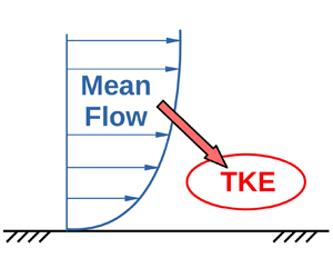
Figure 1. Schematic showing turbulence deriving its energy from the mean flow.

2.2. Asymptotic average TKE production rate over the thickness $L$ of the shear flow

The TKE production term $P := \langle -u'v'\rangle \partial U/\partial y$ in the viscous (wall) scaling is $P_{+}=P\nu /{U_{\tau }}^{4}$. The average value of $P_{+}$ across the thickness of the shear flow (in the $x$–$y$ plane) is

(2.6)\begin{equation} P_{+{{avg}}}=\frac{1}{L}\int_{0}^{L}P_{+} \, \textrm{d} y=\frac{1}{{Re_{\tau}}}\int_{0}^{{Re_{\tau}}}P_{+} \, \textrm{d}{y_{+}}.\end{equation}

It is a well-known observation that, although $P_{+}$ reaches peak value in the buffer layer at ${y_{+}}\approx 12$, the contribution of the inertial overlap layer (log region) to the overall production (i.e. the integral in (2.6)) increases with Reynolds number and dominates over the contribution of the buffer-layer region at high Reynolds numbers (Smits, McKeon & Marusic Reference Smits, McKeon and Marusic2011). Physically, this happens because, with increasing Reynolds number, the lower end of the log region is seen to move closer to the wall in the outer scaling $(\eta := y/L)$. Due to this, the buffer-layer region is sandwiched between an increasingly thinner fraction of the flow thickness located adjacent to the wall; the outer end of the log region is seen to remain located at $\eta \approx 0.15$ independent of the flow Reynolds number (Marusic et al. Reference Marusic, Monty, Hultmark and Smits2013). In view of this, one may split the integral in (2.6) into contributions from the buffer-layer, log layer and wake layer regions, and retain only the log and wake contributions in the limit ${Re\rightarrow \infty }$

(2.7)\begin{equation} P_{+{{avg}}}\rightarrow\frac{1}{{Re_{\tau}}} \left[\int_{3\sqrt{{Re_{\tau}}}}^{0.15{Re_{\tau}}}P_{+{{\log}}}\, \textrm{d}{y_{+}}+\int_{0.15{Re_{\tau}}}^{{Re_{\tau}}}P_{+{{wake}}}\, \textrm{d}{y_{+}}\right].\end{equation}

Here, the log region in ZPG TBLs, pipes and channels is taken to begin at a $Re$-dependent wall-normal location $y_{+}=3\sqrt {{Re_{\tau }}}$ (Wei et al. Reference Wei, Fife, Klewicki and McMurtry2005; Marusic et al. Reference Marusic, Monty, Hultmark and Smits2013) beyond the mesolayer and extend up to the $Re$-independent location $\eta =0.15$ or ${y_{+}}=0.15{Re_{\tau }}$. The wake region occupies the remaining portion of the flow beyond the log region i.e. $0.15{Re_{\tau }}\leq {y_{+}}\leq {Re_{\tau }}$. For the wake part, TKE production is governed only by the outer length scale $L$ (as in free shear flows, see Tennekes & Lumley Reference Tennekes and Lumley1972; Townsend Reference Townsend1976) so that, $P_{{{wake}}}\sim {U_{\tau }}^{3}/L$ or $P_{+{{wake}}}=C_{2}/{Re_{\tau }}$, where $C_{2}$ is a dimensionless constant. For the log region, the production term depends on the distance from the wall i.e. $P_{{{\log }}}\sim {U_{\tau }}^{3}/y$ or $P_{+{{\log }}}=C_{1}/{y_{+}}$ (Tennekes & Lumley Reference Tennekes and Lumley1972; Townsend Reference Townsend1976; Davidson Reference Davidson2015), $C_{1}$ being a dimensionless constant. Substituting the expressions for $P_{+{{wake}}}$ and $P_{+{{\log }}}$ into (2.7) and simplifying yields

(2.8)\begin{equation} P_{+{{avg}}}\rightarrow\frac{1}{{Re_{\tau}}} \left[C_{3}+C_{1}\ln{\sqrt{{Re_{\tau}}}}\right],\end{equation}

where $C_{3}=-2.9957C_{1}+0.85C_{2}$. In order to obtain the correct asymptotic limiting form of (2.8), one needs to consider the $Re$-dependence of the fractional change $\textrm {d}P_{+{{avg}}}/P_{+{{avg}}}$. This may be easily done by differentiating (2.8) with respect to ${Re_{\tau }}$ and dividing the result by (2.8). With some simplifications, this exercise yields

(2.9)\begin{equation} \frac{\textrm{d}P_{+{{avg}}}}{P_{+{{avg}}}}\rightarrow \left[{-}1+\frac{C_{1}}{2(C_{3}+C_{1}\ln\sqrt{{Re_{\tau}}})}\right] \frac{\textrm{d}{Re_{\tau}}}{{Re_{\tau}}},\end{equation}

where the square bracket tends to $-1$ in the limit ${Re_{\tau }\rightarrow \infty }$ (or ${Re\rightarrow \infty }$). Therefore, (2.9) asymptotically becomes

(2.10)\begin{equation} \frac{\textrm{d}P_{+{{avg}}}}{P_{+{{avg}}}}\rightarrow- \frac{\textrm{d}{Re_{\tau}}}{{Re_{\tau}}}.\end{equation}

This shows that

(2.11)\begin{equation} P_{+{{avg}}}\rightarrow\frac{1}{{Re_{\tau}}}\text{ or } P_{{{avg}}}\rightarrow\frac{{U_{\tau}}^{3}}{L}.\end{equation}

Thus, the rate of TKE production averaged over the thickness of the shear flow asymptotes to ${U_{\tau }}^{3}/L$ in the limit ${Re\rightarrow \infty }$ (or ${Re_{\tau }\rightarrow \infty }$). Notice that the asymptotic value of $P_{{{avg}}}$ effectively scales as $P_{{{wake}}}$, implying that the functional form of the mean velocity profile in the inertial overlap layer (assumed to be logarithmic in this derivation) appears to be irrelevant in the asymptotic sense.

Substituting (2.6) and (2.11) in (2.5) shows that

(2.12)\begin{equation} \int_{0}^{{Re_{\tau}}}\frac{{\rm D}U_{+}^{2}}{{\rm D}{t_{+}}} \, \textrm{d}{y_{+}}\rightarrow\text{const}.,\end{equation}

in the limit ${Re\rightarrow \infty }$ (or ${Re_{\tau }\rightarrow \infty }$). Furthermore, we note that the limits of integration on the left side of (2.12) are independent of time (or movement along a streamline) in the limit ${Re\rightarrow \infty }$ (or ${Re_{\tau }\rightarrow \infty }$). This is so because, for pipes and channels, the mean-flow streamlines are parallel to the wall and coincident with the iso-${y_{+}}$ lines. Therefore, the limits of integration on the left side of (2.5) do not change if one moves along a mean streamline. For ZPG TBLs, this condition is satisfied only at high Reynolds numbers, as shown by Dixit & Ramesh (Reference Dixit and Ramesh2018). Therefore, in the limit ${Re\rightarrow \infty }$ (or ${Re_{\tau }\rightarrow \infty }$), the operators $D/D{t_{+}}$ and $\int$ in (2.12) commute for all flows. Note that the use of asymptotic BCs $U(y=L)={U_{\infty }}$ and $V(y=L)=0$ – common to all flows in the limit ${Re\rightarrow \infty }$ – is implicit in the commutation of operators. With this, (2.12) asymptotically becomes

(2.13)\begin{equation} \frac{{\rm D}}{{\rm D}{t_{+}}}\int_{0}^{{Re_{\tau}}}U_{+}^{2}\, \textrm{d}{y_{+}}\rightarrow\textrm{const}.\end{equation}

Kinematic momentum rate of the shear flow in the $x$–$y$ plane (per unit width for ZPG TBLs and channels, and per unit circumference for pipes) is given by

(2.14)\begin{equation} M := \int_{0}^{L}U^{2}\,\textrm{d} y=\nu{U_{\tau}} \int_{0}^{{Re_{\tau}}}U_{+}^{2}\, \textrm{d}{y_{+}}. \end{equation}

Here, $U=U(y)$ is the mean velocity profile at the streamwise location $x$. Also, the quantities ${U_{\tau }}$, $M$ and $L$ are functions of the streamwise coordinate $x$. However, we omit explicit mention of $x$ with an understanding that the quantities being considered are localised in the streamwise direction unless specified otherwise. Substituting (2.14) in (2.13) yields

(2.15)\begin{equation} \frac{{\rm D}}{{\rm D} {t_{+}}}\left(\frac{M}{\nu{U_{\tau}}}\right) \rightarrow\textrm{const}.\end{equation}

Equation (2.15) now needs to be integrated with respect to time.

2.3. Most efficient energy extracting eddies and the asymptotic universal skin friction scaling law

It is well known that the largest eddies of a wall-bounded turbulent shear flow have sizes of order $L$ and their velocity scale is ${U_{\tau }}$. These eddies are the most efficient towards extracting the SMFKE and transferring it to the low-wavenumber end of the turbulence cascade (Tennekes & Lumley Reference Tennekes and Lumley1972; Davidson Reference Davidson2015). The lifetime of these large eddies – the so-called ‘large-eddy’ turnover time – can be estimated as the ratio of their kinetic energy content ($\sim {U_{\tau }}^{2}$) and dissipation rate ($\sim {U_{\tau }}^{3}/L$). The lifetime of large eddies is therefore of the order of $L/{U_{\tau }}$ (Tennekes & Lumley Reference Tennekes and Lumley1972; Lozano-Durán & Jiménez Reference Lozano-Durán and Jiménez2014; Rouhi, Piomelli & Geurts Reference Rouhi, Piomelli and Geurts2016; Kwon & Jiménez Reference Kwon and Jiménez2021). Note that, the time scale of advection of large eddies past a fixed probe in experiments is $L/{U_{\infty }}$ and is commonly referred to as the ‘boundary layer’ turnover time (Hutchins et al. Reference Hutchins, Nickels, Marusic and Chong2009; Mathis et al. Reference Mathis, Hutchins and Marusic2009). This is distinct from the lifetime or turnover time $L/{U_{\tau }}$ of the large eddies. In viscous units, the large-eddy turnover time is simply equal to the friction Reynolds number i.e. $(L/{U_{\tau }}){U_{\tau }}^{2}/\nu ={Re_{\tau }}$. This is expected because the Reynolds number may be interpreted as the ratio of the largest to smallest (viscous) time scales in the flow (Tennekes & Lumley Reference Tennekes and Lumley1972). We now integrate (2.15) over one large-eddy turnover time (${t_{+}}$ from $0$ to ${Re_{\tau }}$) to obtain the SMFKE lost by the mean flow (or the TKE input at the largest flow scales of the cascade), over its complete wall-normal extent, during the lifetime of a typical large eddy. This yields

(2.16)\begin{equation} \frac{M}{\nu{U_{\tau}}}\sim{Re_{\tau}}.\end{equation}

Writing ${U_{\tau }}$ and $L$ in (2.16) in dimensionless form using $M$ and $\nu$ leads to the asymptotic, universal skin friction scaling law

(2.17)\begin{equation} {\widetilde{U}_{\tau}}\sim{\widetilde{L}}^{{-}1/2},\end{equation}

where ${\widetilde {L} := LM/\nu ^{2}}$ and ${\widetilde {U}_{\tau } := U_{\tau }\nu /M}$. Note that ${\widetilde {L}}$ is in fact Reynolds number and ${\widetilde {U}_{\tau }}$ is dimensionless skin friction, both based on a new velocity scale $M/\nu$ obtained from the governing dynamics. Also note that the present asymptotic, universal $-1/2$-power scaling law (2.17) is identical to the asymptotic $-1/2$-power scaling law derived earlier by Dixit et al. (Reference Dixit, Gupta, Choudhary, Singh and Prabhakaran2020) only for ZPG TBLs (see (A1) of Appendix A). It is re-emphasised, that the present derivation is more general, covers ZPG TBLs, pipes as well as channels at once and the scaling law (2.17) is therefore deemed universal.

2.4. Dynamically consistent velocity scale $M/\nu$

Conceptual implications of the present derivation of the asymptotic, universal $-1/2$ power scaling law for skin friction (2.17) are quite revealing. First, the derivation shows that the scaling law is universal and holds for ZPG TBLs, pipes as well as channels. Secondly, for the dimensionless representation of the behaviour of skin friction with Reynolds number, $M/\nu$ emerges as a new velocity scale that is consistent with the governing dynamical equations. This is very significant because, traditionally, the skin friction data in ZPG TBLs are ‘scaled’ using the free-stream velocity ${U_{\infty }}$ (Fernholz & Finley Reference Fernholz and Finley1996; Dixit et al. Reference Dixit, Gupta, Choudhary, Singh and Prabhakaran2020). For pipes and channels, the bulk or the mass-averaged velocity $U_{b}$ is used (McKeon et al. Reference McKeon, Zagarola and Smits2005; Dixit et al. Reference Dixit, Gupta, Choudhary, Singh and Prabhakaran2021). These velocity scales have been in wide use perhaps because of their role either as the outer velocity BC (${U_{\infty }}$ in TBLs) or as a practical convenience ($U_{b}$ is proportional to flow rate through the pipe). Given the velocity scale, dimensionless skin friction (${C_{f}}$ in TBLs and channels, or $\lambda$ in pipes), and Reynolds number (${Re_{\theta }}$ in ZPG TBLs or ${Re_{L}}$ in channels and pipes, both to be defined shortly), in their traditional from, are simply a consequence of the dimensional analysis following Buckingham's Pi theorem. It is important to realise that these traditional velocity scales are not intrinsic to the governing dynamics but more akin to BCs. The preceding sections, for the first time and to the best of our knowledge, provide a single, dynamically consistent velocity scale $M/\nu$ for scaling skin friction in ZPG TBLs, pipes as well as channels. This provides a basis for exploring universality of skin friction scaling amongst these flows.

2.5. Finite-$Re$ model for skin friction

Dixit et al. (Reference Dixit, Gupta, Choudhary, Singh and Prabhakaran2020) have derived a finite-$Re$ model (A2) for skin friction in ZPG TBLs from the asymptotic $-1/2$ power scaling law (A1) as may be seen in Appendix A. The present asymptotic, universal $-1/2$ power scaling law (2.17) is identical to (A1). Therefore, the finite-$Re$ model (A2) readily applies individually to all the flows of the present interest. In view of this, the finite-$Re$ model for each individual flow type reads

(2.18)\begin{equation} {\widetilde{U}_{\tau}}=\frac{A_{1}}{\ln{\widetilde{L}}}{\widetilde{L}}^{\left[-{1}/{2}+{B_{1}}/{\sqrt{\ln{\widetilde{L}}}}\right]}.\end{equation}

Equation (2.18) implies that ${\widetilde {U}_{\tau }}$ is an explicit function of ${\widetilde {L}}$ with the general form

(2.19)\begin{equation} {\widetilde{U}_{\tau}}=F_{1}({\widetilde{L}}),\end{equation}

where the functional form of $F_{1}$ is given by the right side of (2.18). Note that the functional forms of (2.17) and (2.18) remain identical in the case of ZPG TBLs, pipes and channels. However, the values of the finite-$Re$ model coefficients in (2.18) may be expected to vary from one flow to the other. This is because, at finite Reynolds numbers, the BCs of different flows are not identical. Also, there are geometry-related differences amongst different flows and these could become important, as noted towards the beginning of this section.

As interim summary, we note that the $M$–$\nu$ scaling of skin friction (i.e. the $({\widetilde {L}},{\widetilde {U}_{\tau }})$ space) is a dynamically consistent framework. It contains an asymptotic, universal $-1/2$-power scaling law (2.17) that holds for all flows. There is also a finite-$Re$ model (2.18) which is expected to hold well for individual flows, but may or may not hold well if one attempts a universal description across all types of flows.

4.1. The $M$–$\nu$ scaling for individual flows in the $({\widetilde {L}},{\widetilde {U}_{\tau }})$ space

Figure 3(a) shows the channel flow data of table 1 plotted in the space of ${\widetilde {L}}$ and ${\widetilde {U}_{\tau }}$ variables. Clearly, the data appear to line up along a single curve exhibiting scaling in this space as expected from the theory presented in § 2. The equation of this curve is mathematically given by the finite-$Re$ model (2.18). A least-squares fit (using MATLAB function nlinfit) of this model to the data is shown in figure 3(a). The values of model constants $A_{1}$ and $B_{1}$ are also shown along with the respective $95\,\%$ confidence intervals given parenthetically. Departure of the data from the fitted model is quantified by the root-mean-squared error (RMSE) and is displayed in figure 3(a). Here, RMSE is the square root of the mean squared error, a measure of the spread of the residuals, returned by the MATLAB nlinfit function. To visualise how well the data ‘scale’ in figure 3(a), we compute the percentage deviation of the actual values of ${U_{\tau }}$ with respect to those obtained from the fit of the model. These deviations are shown in figure 3(b). It is clear that almost all the percentage deviations are within $\pm 1\,\%$ which is on par with the measurement uncertainty of skin friction in channel flows (Schultz & Flack Reference Schultz and Flack2013). The root-mean-squared (RMS) value of these percentage deviations is $0.64\,\%$; percentage deviations are squared, averaged and then the square root is taken. Figure 3(c) shows the probability histogram of percentage deviations of figure 3(b). The histogram is narrow and without any noticeable skew. This confirms that the channel flow data scale quite well in the $M$–$\nu$ scaling framework, and the finite-$Re$ model (2.18) accurately describes the variation in the data. Figures 4 and 5 show results of the same processing carried out on the pipe and ZPG TBL data, respectively. The conclusions are largely the same. Somewhat increased scatter in the percentage ${U_{\tau }}$ deviations for ZPG TBLs (figure 5b) and a weak skew in the corresponding probability histogram (figure 5c) are attributed to the inherent larger measurement uncertainty of ${U_{\tau }}$ ($\pm 2.5\,\%$) in ZPG TBLs. For pipes and channels, this uncertainty is approximately $\pm 1\,\%$, since there is privilege to infer ${U_{\tau}}$ from accurate pressure drop measurements in fully developed internal flows.

Figure 3. Channel flow skin friction data of table 1. (a) The $M$–$\nu$ scaling framework i.e. the $({\widetilde {L}},{\widetilde {U}_{\tau }})$ space. Solid line shows least-squares fit of the finite-$Re$ model (2.18) to the data. Fitting constants are also shown along with the RMSE for the fit.(b) Percentage deviations in the actual values of ${U_{\tau }}$ with respect to those computed using the finite-$Re$ model fitted in (a). Dashed lines indicate the band of $[-1,1]$ and dashed-dotted lines indicate the band of $[-2.5,2.5]$. RMS value of the percentage deviations is also shown. (c) Probability histogram for the percentage deviations. Probability values for the two bands $[-1,1]$ (dashed lines) and $[-2,2]$ (dashed-dotted lines) are also shown.

Figure 4. Pipe flow skin friction data of table 1. Remaining details same as the caption of figure 3.

Figure 5. ZPG TBL skin friction data of table 2. Remaining details same as the caption of figure 3.

The results of figures 3–5 provide compelling evidence in favour of the theory presented in § 2. Indeed, the $M$–$\nu$ scaling ((2.17) and (2.18)) is seen to scale and describe individual data from ZPG TBLs, pipes as well as channels, to an excellent accuracy. This implies that the functional forms of (2.17) and (2.18) do not depend on the BCs and geometry, as expected from the theory of § 2. It is, however, important to note that the values of model constants $A_{1}$ and $B_{1}$ in (2.18) do in fact vary from one flow to the other. This variation is clear from the values listed in figures 3(a)–5(a), and is most likely to be due to the effects of BCs at finite Reynolds numbers and geometry as discussed in § 2.

4.2. Does $M$–$\nu$ scaling in $({\widetilde {L}},{\widetilde {U}_{\tau }})$ space hold for different flow types taken together?

Figure 6 shows the same processing of the data as for figures 3–5, but this time with the data from all different flow types (tables 1 and 2) put together. Figure 6(a) shows the fit of the finite-$Re$ model (2.18) performed for all the data taken together. RMSE value for the fitted curve in figure 6(a) shows a twofold increase compared with the RMSE values seen in figures 3(a)–5(a). Figure 6(b) shows that most of the deviations remain confined to the band of $\pm 2.5\,\%$ in ${U_{\tau}}$ which is typical of skin friction measurement uncertainties in ZPG TBLs. RMS percentage deviation is $1.69$ which is more than twice the values for individual flows. Differences in the percentage deviations for ZPG TBLs and pipe flow data at high Reynolds numbers are now confined to less than $5\,\%$. Thus, there is some improvement over the disagreement of $7\,\%$ noted earlier for the traditional $({{{\rm Re} _{\theta }}},{{C_{f}}})$ space. This suggests that the $M$–$\nu$ scaling enables somewhat better collapse of all the data from different flows compared with the traditional scaling.

Figure 6. Skin friction data of all the flows listed in tables 1 and 2. Panel (c) shows probability histograms for the percentage deviations for the individual flow types as well as for the complete data. Remaining details same as the caption of figure 3.

However, it is interesting to note that the ZPG TBL deviations in figure 6(b) systematically drift to negative values with increasing Reynolds number. The opposite is true for the pipe flow data. This can be readily seen in figure 6(c) as well where the probability histograms are biased to the right side for pipes and channels, and to the left side for ZPG TBLs. The probability histogram for all the data is therefore rather flat. Hence, one may conclude that the data from different types of flows do not collapse very well onto each other and hence, onto the curve of the fitted model. Trends in figure 6(b) imply that, with increasing Reynolds number, the ZPG TBL data in figure 6(a) progressively deviate downward with respect to the model curve while the pipe (and channel) data deviate upward. Since the asymptotic dynamical framework is universal (see § 2), the persistent discrepancies in the $M$–$\nu$ scaling trends must come from aspects of different flows that are outside the scope of the theory of § 2. Therefore, these discrepancies could well be related to the differences in the BCs at finite Reynolds numbers and geometry amongst different flow types as discussed before in § 2. If indeed, this were the case, absorbing these differences into the framework of $M$–$\nu$ scaling appears to be the key to universal scaling of skin friction.

5.1. Clauser shape factor $G$

An objective integral measure of the fullness of the mean velocity profile is its shape factor. As pointed out by Clauser (Reference Clauser1956), mean velocity profiles of ZPG TBLs exhibit self-similarity in defect coordinates. Therefore, it is appropriate to define shape factor based on defect profiles such that it would be constant for a given self-similar (defect scaled) TBL flow. Clauser defines this shape factor as

(5.1)\begin{equation} G := \int_{0}^{\infty}\left(\frac{U-{U_{\infty}}}{{U_{\tau}}}\right)^{2}\, \textrm{d}\left(\frac{y}{\varDelta}\right),\end{equation}

where $\varDelta$ is the integral thickness based on mean velocity profiles in defect scaling

(5.2)\begin{equation} \varDelta := \int_{0}^{\infty}\left(\frac{U-{U_{\infty}}}{{U_{\tau}}}\right)\, \textrm{d} y.\end{equation}

Further, $G$ and ${C_{f}}$ are related (Clauser Reference Clauser1956) to the conventional shape factor $H$ (ratio of displacement to momentum thickness) by

(5.3)\begin{equation} H=\left(1-G\sqrt{{C_{f}}/2}\right)^{{-}1}.\end{equation}

Note that (5.1)–(5.3) can be readily applied to turbulent pipes and channels as well. Since the mean velocity profile fullness increases (defect decreases) in the order ZPG TBL, pipe and channel (see Monty et al. Reference Monty, Hutchins, Ng, Marusic and Chong2009), $G_{{{ZPG\ TBL}}}>G_{{{pipe}}}>G_{{{channel}}}$ at matched ${Re_{\tau }}$.

For ZPG TBLs, $G\approx 6.8$ at moderate and high Reynolds numbers (Clauser Reference Clauser1956). To compare the fullness of mean velocity profiles from different flows, this asymptotic value of $G$ for ZPG TBLs could be taken as an arbitrary, yet useful, reference i.e. $G_{{{ref}}}=6.8$. With this, the departure of the fullness of a mean velocity profile (in any flow) from the reference fullness could be quantified by $(G-G_{{{ref}}})/G_{{{ref}}}$, or simply by the ratio ${G/G_{{{ref}}}}$. Using (5.3), ${G/G_{{{ref}}}}$ may be expressed as

(5.4)\begin{equation} \frac{G}{G_{{{ref}}}}=\frac{{U_{\infty}}}{G_{{{ref}}}{U_{\tau}}} \left(\frac{H-1}{H}\right)=\frac{{\widetilde{U}_{\infty}}}{G_{{{ref}}}{\widetilde{U}_{\tau}}} \left(\frac{H-1}{H}\right),\end{equation}

where ${\widetilde {U}_{\infty }}={U_{\infty }\nu /M}$. Note that ${\widetilde {U}_{\infty }}$ and $H$ are known parameters from a measured or computed mean velocity distribution, and $G_{{{ref}}}=6.8$ is a constant. Thus, ${G/G_{{{ref}}}}$ itself is a function of ${\widetilde {U}_{\tau }}$.

5.2. Universal, semi-empirical $M$–$\nu$–$G$ scaling and finite-$Re$ model: the $({\widetilde {L}}',\widetilde {U}_{\tau }')$ space

Momentum rate $M$ does, to some extent, capture the fullness of a mean velocity profile. This explains why the $M$–$\nu$ scaling is able to reduce the disagreement in ${U_{\tau }}$ from $7\,\%$ in figure 2 to $5\,\%$ in figure 6 (see § 4.2). However, a correct measure of the fullness needs to view the mean velocity profile with respect to the free stream (Clauser Reference Clauser1956). Therefore, comparing the definitions (2.14) and (5.1), it is clear that $M$ cannot be a complete measure of the fullness of the mean velocity profiles. Therefore, the $M$–$\nu$ scaling needs a formal correction to account for the differences in the fullness of the mean velocity profiles. In view of the discussion in the previous sections, such a correction should be based on $G$ (or ${G/G_{{{ref}}}}$) if one wishes to obtain a universal scaling of skin friction for all flows.

We now attempt to introduce this empirical correction. The expectation is that this $M$–$\nu$–$G$ scaling would lead to a much better collapse of the data from all the flows than the $M$–$\nu$ scaling alone. Towards this, we propose an empirical transformation of the variables ${\widetilde {L}}$ and ${\widetilde {U}_{\tau }}$ using correction factors that are functions of the ratio ${G/G_{{{ref}}}}$. Specifically, we assume the correction factors to have a power-law functional form and define our new shape-factor-corrected variables as

(5.5)\begin{gather} {\widetilde{U}_{\tau}}' := {\widetilde{U}_{\tau}}(G/G_{{{ref}}})^{p}, \end{gather}

(5.6)\begin{gather}{\widetilde{L}}' := {\widetilde{L}}(G/G_{{{ref}}})^{q}, \end{gather}

where $p$ and $q$ ($p\neq q$, in general) are empirical constants. Note that the original dimensionless variables ${\widetilde {L}}$ and ${\widetilde {U}_{\tau }}$ (of $M$–$\nu$ scaling) have been respectively transformed to the new variables ${\widetilde {L}}'$ and $\widetilde {U}_{\tau }'$ (of $M$–$\nu$–$G$ scaling). We expect data from all flows to scale universally in the new $({\widetilde {L}}',\widetilde {U}_{\tau }')$ space.

Two points related to the $M$–$\nu$–$G$ scaling need some emphasis. First, since one major purpose of the correction is to account for differences in BCs at finite Reynolds numbers, it makes sense to apply the correction only to the finite-$Re$ model (2.18). That is, we only seek to construct a universal finite-$Re$ model, and do not attempt to derive an asymptotic scaling law in the $M$–$\nu$–$G$ scaling. This is because, at present, we are not aware of a theoretical approach which would include $G$ into the asymptotic analysis of $M$–$\nu$ scaling (§§ 2.1–2.3) without resorting to empirical scaling descriptions such as the defect scaling. Second, we propose that the functional form of the (supposedly) universal finite-$Re$ model should be the same as that of (2.18). That is, the original variables ${\widetilde {L}}$ and ${\widetilde {U}_{\tau }}$ in (2.18) may simply be replaced by the new variables ${\widetilde {L}}'$ and $\widetilde {U}_{\tau }'$, respectively. The basis for this proposal is that the universal model should correctly reduce to (2.18) for individual flows.

In view of the above, the (supposedly) universal finite-$Re$ model in $M$–$\nu$–$G$ scaling, reads

(5.7)\begin{equation} {\widetilde{U}_{\tau}}'=\frac{A'_{1}}{\ln{\widetilde{L}}'}{\widetilde{L}}'^{\left[B'_{0}+{B'_{1}}/{\sqrt{\ln{\widetilde{L}}'}}\right]},\end{equation}

where $A'_{1}$, $B'_{0}$ and $B'_{1}$ are model constants. To check the reduction of (5.7) to (2.18) for only ZPG TBLs, note that ${G/G_{{{ref}}}}\approx 1$ already. Therefore, the functional form of (5.7) reduces to that of (2.18), as expected. Also, the fitting constant $B'_{0}$ is known to be $-1/2$ for ZPG TBLs from the universal asymptotic scaling law (2.17). Therefore, with $A'_{1}=A_{1}$, $B'_{0}=-1/2$ and $B'_{1}=B_{1}$, (5.7) readily reduces to (2.18) for ZPG TBLs. Further, note that ${G_{{{ref}}}}=6.8$ is just an arbitrary reference value, chosen to be equal to the value of $G$ in ZPG TBLs. If one wishes to consider how (5.7) reduces for only pipes (channels), then the value of ${G_{{{ref}}}}$ should be chosen to be equal to the asymptotic value of $G$ in pipes (channels), so that ${G/G_{{{ref}}}}\approx 1$ for pipes (channels). With this, the fitting constant $B'_{0}$ is again known to be $-1/2$ from the universal asymptotic scaling law (2.17). Then, with $A'_{1}=A_{1}$, $B'_{0}=-1/2$ and $B'_{1}=B_{1}$, (5.7) readily reduces to (2.18) applicable to pipes (channels).

The aim of (5.7) is to universally describe skin friction data in all the flows taken together. Hence, the correction factor is chosen with a common normalisation using ${G_{{{ref}}}}=6.8$. As may be seen from tables 1 and 2, ${G/G_{{{ref}}}}\neq 1$ for all the data. Hence, the value of the fitting constant $B'_{0}$ in (5.7), in this case, cannot be specified to be $-1/2$; in fact, it is expected to be different from it. This is because the asymptotic, universal $-1/2$ power scaling law (2.17) formally holds only in $({\widetilde {L}},{\widetilde {U}_{\tau }})$ space (i.e. $M$–$\nu$ scaling) and not in the new $({\widetilde {L}}',\widetilde {U}_{\tau }')$ space (i.e. $M$–$\nu$–$G$ scaling). It is re-emphasised that the proposed corrections, although guided by the data and the physical understanding outlined before, are purely empirical in nature. The contention is that the finite-$Re$ model in $M$–$\nu$–$G$ scaling (5.7), universally describes all the data from different types of flows to an approximation significantly better than (2.18).

In order to complete the universal finite-$Re$ model (5.7), one needs to determine the values of five constants namely $p$, $q$, $A'_{1}$, $B'_{0}$ and $B'_{1}$. Towards this, we use the following approach involving simple optimisation and model curve fitting. First, we arbitrarily select the values for $p$ and $q$, and compute ${\widetilde {L}}'$ and $\widetilde {U}_{\tau }'$ for the data. Next, we perform a nonlinear least-squares fit (using the MATLAB function nlinfit) of the shape-factor-corrected finite-$Re$ model (5.7) to the data, and obtain the RMSE of the data with respect to the fitted curve. Finally, we systematically and independently vary the values of $p$ and $q$ each over the (arbitrary) range $-10$ to $10$, and for each pair of values $(p,q)$, we repeat the above procedure and monitor the RMSE value. The pair $(p,q)$ exhibiting the minimum RMSE for the fitted model is considered as the optimised pair $(p_{{{opt}}},q_{{{opt}}})$, and the values of $A'_{1}$, $B'_{0}$ and $B'_{1}$ corresponding to this fit of the model are finalised for further analysis.

Figure 7(a) shows all the data plotted in the space $({\widetilde {L}}',\widetilde {U}_{\tau }')$ of $M$–$\nu$–$G$ scaling. The least-squares fit of (5.7) to all the data is shown by the solid line. Note that the optimisation and curve-fitting process mentioned in the preceding paragraph goes back and forth between the data and curve fit in figure 7(a). The optimum values of $p$ and $q$ in (5.5) and (5.6) turn out to be $p_{{{opt}}}=1.006$ and $q_{{{opt}}}=-1.489$, as shown in figure 7(a). Also, the values of the constants in (5.7) turn out to be $A_{1}'=2.2058$, $B_{0}'=-0.4716$ and $B_{1}'=-0.3147$. A careful look at figures 6(a) and 7(a) indicates discernible improvement in data collapse when the shape factor correction is included i.e. switching over from $M$–$\nu$ scaling to $M$–$\nu$–$G$ scaling. Figures 6(b) and 7(b) quantify this improvement. The RMSE with reference to the corresponding finite-$Re$ model improves significantly by almost an order of magnitude from $0.01736$ (figure 6b) to $0.00665$ (figure 7b). It is interesting to note that $B_{0}'=-0.4716$ with the inclusion of the shape factor effect (see figure 7b). As discussed before, this value is indeed different from the asymptotic universal scaling-law exponent of $-1/2$. Figure 7(b) demonstrates that the shape factor correction dramatically reduces the differences in the trends noted earlier in figure 6(b). This is clear from the reduction in the RMS percentage deviation in ${U_{\tau }}$ by more than a factor of two from $1.72$ (figure 6b) to $0.80$ (figure 7b). Figure 7(c) reflects this dramatic improvement in the data collapse in terms of clustering of the probability histograms for all types of flows around the percentage ${U_{\tau }}$ deviation value of zero. Figure 7(c) is to be contrasted with figure 6(c).

Figure 7. Skin friction data of all the flows listed in tables 1 and 2. (a) The $({\widetilde {L}}',\widetilde {U}_{\tau }')$ space. Solid line shows least-squares fit of the universal finite-$Re$ model (5.7) to the data. Panel (c) shows probability histograms for the percentage deviations for the individual flow types as well as for the complete data. Remaining details same as the caption of figure 3.

One caveat needs to be noted before closing this discussion. Percentage deviations of the four highest Reynolds number ZPG TBL data (the last four data points of ZPG TBL:Exp4 data set in table 2) are close to $-2.5\,\%$, as seen in figure 7(b). For the pipe flow data, however, these deviations remain very close to $+1\,\%$ even at the highest Reynolds numbers. This discrepancy, although largely acceptable for engineering calculations, presents a hurdle in inferring a true tendency towards asymptotic $M$–$\nu$–$G$ scaling of the skin friction from the experimental data on ZPG TBLs and pipes. The discrepancy is most likely to be related to the method of measuring skin friction in experiments. Unfortunately, most skin friction measurements in high-$Re$ ZPG TBLs (including ZPG TBL:Exp4 data set) rely on a Clauser chart or on Fernholz's correlation (Vallikivi et al. Reference Vallikivi, Hultmark and Smits2015). These methods essentially rely on the universal log law for mean velocity variation (Dixit et al. Reference Dixit, Gupta, Choudhary, Singh and Prabhakaran2020). Pipe flows, on the other hand, allow accurate direct measurement of skin friction through pressure drop measurement. It is known that the log-law-based friction factor models in pipe flows need adjustment of constants at extreme Reynolds numbers (McKeon et al. Reference McKeon, Zagarola and Smits2005; Dixit et al. Reference Dixit, Gupta, Choudhary, Singh and Prabhakaran2021). Whether such an adjustment is required for Fernholz's correlation in ZPG TBLs is an open question that can only be addressed by direct measurements of skin friction at high Reynolds numbers using techniques such as oil film interferometry. In view of this, there is no way to assess the inherent realistic uncertainty in the measured skin friction for the four highest Reynolds number ZPG TBL data of figure 7(b). Future experiments with direct measurement of skin friction in high-$Re$ ZPG TBLs should be able to settle this issue and assess the true asymptotic applicability of $M$–$\nu$–$G$ scaling in the limit ${Re\rightarrow \infty }$.

Notwithstanding this, and within the uncertainties of the data, the results of figure 7 provide strong support in favour of the universal $M$–$\nu$–$G$ scaling and finite-$Re$ model (5.7) for skin friction in all flows at finite Reynolds numbers.

5.3. Converting from $({\widetilde {L}}',\widetilde {U}_{\tau }')$ space to three-dimensional $({\widetilde {L}},{G/G_{{{ref}}}},{\widetilde {U}_{\tau }})$ space

Equation (5.7) universally (for all flows) relates the variables ${\widetilde {L}}'$ and $\widetilde {U}_{\tau }'$ in the $M$–$\nu$–$G$ scaling according to the general functional form

(5.8)\begin{equation} {\widetilde{U}_{\tau}}'=F_{2}({\widetilde{L}}'),\end{equation}

so that $\widetilde {U}_{\tau }'$ is a function of a single variable ${\widetilde {L}}'$. Equation (5.8) may be converted back to the original variables ${\widetilde {L}}$ and ${\widetilde {U}_{\tau }}$ along with the third variable ${G/G_{{{ref}}}}$ that amounts to the shape factor correction. Expanding (5.7) using the definitions (5.5) and (5.6), and rearranging yields

(5.9)\begin{equation} {\widetilde{U}_{\tau}}=\frac{A'_{1}}{\ln[{\widetilde{L}}({G/G_{{{ref}}}})^{q}]} [{\widetilde{L}}({G/G_{{{ref}}}})^{q}]^{\left[B'_{0}+\frac{B'_{1}}{\sqrt{\ln [{\widetilde{L}}({G/G_{{{ref}}}})^{q}]}}\right]}({G/G_{{{ref}}}})^{{-}p}.\end{equation}

Equation (5.9) shows that ${\widetilde {U}_{\tau }}$ is a function of two variables, namely ${\widetilde {L}}$ and ${G/G_{{{ref}}}}$, wherein ${G/G_{{{ref}}}}$ in turn depends on ${\widetilde {U}_{\tau }}$ according to (5.4). Therefore, the universal finite-$Re$ model (5.7) translates to an implicit (in ${\widetilde {U}_{\tau }}$) expression of the general form

(5.10)\begin{equation} {\widetilde{U}_{\tau}}=F_{3}({\widetilde{L}},{G/G_{{{ref}}}}),\end{equation}

where the functional form of $F_{3}$ is given by the right side of (5.9).

Figure 8 shows all the data plotted in the three-dimensional space $({\widetilde {L}},{G/G_{{{ref}}}},{\widetilde {U}_{\tau }})$. Also plotted is the surface given by (5.9) with values of all the empirical constants the same as those obtained in the previous section. It is clear that the data points conform very well to the surface, implying universal scaling according to (5.7) or (5.9).

Figure 8. Skin friction data in the three-dimensional space of ${\widetilde {L}}$, ${G/G_{{{ref}}}}$ and ${\widetilde {U}_{\tau }}$ variables as per (5.9) and (5.8). Shading represents the surface given by (5.9) using $p=p_{{{opt}}}=1.006$, $q=q_{{{opt}}}=-1.489$, $A_{1}'=2.2058$, $B_{0}'=-0.4716$ and $B_{1}'=-0.3147$ as shown earlier in figure 7(a). Panel (b) shows an almost along-the-surface view of the same data as in (a). This panel confirms tight collapse of the data points onto the surface given by (5.9).