


1 Introduction
1.1 The existence and detection of UMZ
The uniform-momentum zone (UMZ) is an instantaneous phenomenon that has been found in the presence of wall-bounded flows. The existence of the UMZ was first found in the experiment of a turbulent boundary layer (TBL) by Meinhart & Adrian (Reference Meinhart and Adrian1995) who observed large regions of relatively uniform streamwise velocities. This enables the detection of the UMZ from the probability density functions (PDF) of the instantaneous streamwise velocity. Distinct peaks on the PDFs represent large regions of the flow developing downstream at relatively constant velocities, namely the zone modal velocities. Kwon et al. (Reference Kwon, Philip, de Silva, Hutchins and Monty2014) and Yang, Hwang & Sung (Reference Yang, Hwang and Sung2016) studied the innermost UMZ in a turbulent channel flow, called the quiescent core region. The UMZ/core boundary was defined by a fixed threshold velocity at 95 % of the centreline velocity ( $u_{\unicode[STIX]{x1D705}}/U_{CL}=0.95$), suggested by the PDF of the modal velocities over time. Kwon et al. (Reference Kwon, Philip, de Silva, Hutchins and Monty2014) reported that the quiescent core of the channel is very large, and can occupy approximately
  $\frac{3}{4}$ of the channel height on average. The channel core exhibited significant thinning, thickening and meandering behaviour; it occasionally extended very close to the channel walls and left the centreline outside the core (
 ${\approx}7\,\%$ of the time overall). A recent study by Fan et al. (Reference Fan, Xu, Yao and Hickey2019) proposed a new method to identify the internal shear layers bounding the UMZs. The method does not require user-defined parameters as for the PDF approach to UMZ identification and is insensitive to the streamwise domain length.
The UMZ interface demarcates the neighbouring UMZs with strong shear originated from concentrated patches of spanwise vortices observed by Meinhart & Adrian (Reference Meinhart and Adrian1995) and Adrian, Meinhart & Tompkins (Reference Adrian, Meinhart and Tompkins2000). These organised vortical structures at the UMZ interface were responsible for ejections ( $Q2$ events) and sweeps (
 $Q4$ events) around the interface (Tomkins & Adrian Reference Tomkins and Adrian2003; Ganapathisubramani, Longmire & Marusic Reference Ganapathisubramani, Longmire and Marusic2003). The retrograde vortices frequently appeared at the backbone of the prograde vortices, matched the experimental observation of Adrian et al. (Reference Adrian, Meinhart and Tompkins2000) and Yang, Meng & Sheng (Reference Yang, Meng and Sheng2001). In Yang et al. (Reference Yang, Hwang and Sung2016), the population of prograde and retrograde spanwise vortices showed a local maximum and minimum in the vicinity of the interface respectively. Across the UMZ interface, an abrupt jump in the streamwise velocity accompanied by local maximum spanwise vorticity and decay of turbulent intensity was observed in the channel (Kwon et al. Reference Kwon, Philip, de Silva, Hutchins and Monty2014; Yang et al. Reference Yang, Hwang and Sung2016), pipe (Kwon Reference Kwon2016; Yang, Hwang & Sung Reference Yang, Hwang and Sung2017) and TBL (de Silva et al. Reference de Silva, Philip, Hutchins and Marusic2017).
de Silva, Hutchins & Marusic (Reference de Silva, Hutchins and Marusic2016) investigated multiple UMZs in TBL and found the number of UMZs increasing log-linearly with the Reynolds number. The thickness of the UMZs was found to be increasing as a function of the distance from the wall, forming a hierarchical distribution of UMZs in the boundary layer. The hierarchical structural arrangement matched the scaling model by Perry & Chong (Reference Perry and Chong1982) described in Marusic & Monty (Reference Marusic and Monty2019). de Silva et al. (Reference de Silva, Philip, Hutchins and Marusic2017) found the velocity jump at the interfaces as a function of the wall-normal distance, being larger nearer the wall. The thickness of the UMZ interface themselves was also a function of the distance from the wall, being thicker further away from the wall. The hierarchical scaling of the UMZs with thinner zones and larger velocity jumps across the sharpened interface nearer the wall was used by Bautista et al. (Reference Bautista, Ebadi, White, Chini and Klewicki2019) for their UMZ-vortical fissure model in TBL. Turbulence statistics were largely reproduced using a discrete step-like initial velocity profile modelled from the UMZ hierarchical distribution. Laskari et al. (Reference Laskari, de Kat, Hearst and Ganapathisubramani2018) investigated the evolution of the UMZ and showed that when the number of UMZ increases, all existing UMZs become thinner and move away from the wall with a higher modal velocity to compensate for the new zones.
The UMZ interface folds intensively with bulges and valleys similar to the large-scale engulfment of the turbulent/non-turbulent interface (TNTI) (Kwon et al. Reference Kwon, Philip, de Silva, Hutchins and Monty2014). The contortion of the UMZ interfaces, which are iso-surfaces of the streamwise velocity, is a manifestation of the large-/very-large-scale motions (LSM/VLSM) in wall turbulence (Saxton-Fox & McKeon Reference Saxton-Fox and McKeon2017; Yang et al. Reference Yang, Hwang and Sung2017). Saxton-Fox & McKeon (Reference Saxton-Fox and McKeon2017) reconstructed the velocity field of TBL using an LSM model and recreated the classical characteristics of UMZs such as the large-scale bulges on the UMZ interface. Yang et al. (Reference Yang, Hwang and Sung2016) measured the two-dimensional (2-D) contortion of the UMZ interface by comparing the length of the UMZ interface per unit length in the streamwise and spanwise direction of the channel. The UMZ interface was found, on average, to be longer in the spanwise direction, so that the interfaces are wavier and the LSMs meander with higher frequencies in the spanwise direction than in the streamwise direction. de Silva et al. (Reference de Silva, Philip, Hutchins and Marusic2017) found the streamwise length of the UMZ interfaces to be longer when departing from the wall, and they exhibited a power-law behaviour with fractal scaling at a constant exponent for all interfaces within the TBL. Recent statistical results by Kevin & Hutchins (Reference Kevin and Hutchins2019) also reported that the meandering of the LSM/contortion of the UMZ interface intensifies with increasing distance from the wall. Multiple UMZs are demarcated by UMZ interfaces with similar large-scale engulfment from meandering/contortion and small-scale entrainment by local patches of vortices. The interface resembles the TNTI, forming a multi-layered structural arrangement with hierarchical scaling in wall turbulence (Perry & Chong Reference Perry and Chong1982; Bautista et al. Reference Bautista, Ebadi, White, Chini and Klewicki2019; Marusic & Monty Reference Marusic and Monty2019).
To the authors’ best of knowledge, the characteristics of multiple UMZs and their interfaces have been studied only in TBL (de Silva et al. Reference de Silva, Hutchins and Marusic2016, Reference de Silva, Philip, Hutchins and Marusic2017; Laskari et al. Reference Laskari, de Kat, Hearst and Ganapathisubramani2018). The first part of this study investigates many of these characteristics in the pipe flow via conditional averaging. The results are extensively compared with the multiple UMZs in TBL and the single quiescent core region in a channel to deduce differences and similarities in wall turbulence. The second part of this study investigates the UMZ interface in three dimensions. The attachment between UMZ interfaces and vortical structures are observed three-dimensionally and in the azimuthal direction of the pipe. The dynamical attachment is shown for the first time for its role in the contortion of UMZ interface. The 3-D contortion/meandering of the UMZ/LSM and its behaviour with wall distance is measured statistically. The bulges and valleys on the UMZ interface are investigated with the  $Q4$ sweep and
  $Q2$ ejection events. The reported footprint of the LSM away from the wall (Rao, Narasimha & Narayanan Reference Rao, Narasimha and Narayanan1971; Metzger & Klewicki Reference Metzger and Klewicki2001; Jiménez, del Álamo & Flores Reference Jiménez, del Álamo and Flores2004) in the near-wall cycle is investigated in the UMZ aspect. Statistics are computed to show the modulation of the near-wall bursting events by the LSM in the centre region of the pipe (Hutchins & Marusic Reference Hutchins and Marusic2007a,Reference Hutchins and Marusicb; Marusic & Hutchins Reference Marusic and Hutchins2008; Chung & McKeon Reference Chung and McKeon2010; McKeon & Sharma Reference McKeon and Sharma2010; Baars, Hutchins & Marusic Reference Baars, Hutchins and Marusic2017). The asymmetry of the large-scale modulation (Agostini & Leschziner Reference Agostini and Leschziner2014, Reference Agostini and Leschziner2016) is measured along the wall-normal direction using the 3-D UMZ interfaces.
2 Numerical simulation
This study investigates the direct numerical simulation (DNS) data of a fully developed turbulent pipe flow at a friction Reynolds number of  $Re_{\unicode[STIX]{x1D70F}}\approx 500$. The DNS data are generated by a massively paralleled MPI (Message Passing Interface) code, Nek5000 (Fischer, Lottes & Kerkemeier Reference Fischer, Lottes and Kerkemeier2008) using the spectral element method (SEM). The incompressible Navier–Stokes equations are solved in Cartesian coordinates to avoid the singularity issue associated with the cylindrical coordinates at the pipe centreline (Jung & Chung Reference Jung and Chung2012; Wang et al. Reference Wang, Orlu, Schlatter and Chung2018). A semi-implicit time scheme solves the viscous terms implicitly using a third-order backward differentiation (BDF3) and the nonlinear terms by a third-order extrapolation (EXT3). The periodic boundary condition was applied in the streamwise direction and the no-slip condition at the pipe wall.
In this study, the streamwise, radial and azimuthal directions of the pipe are denoted by  $x$,
$x$,  $r$ and
  $\unicode[STIX]{x1D703}$ respectively, with wall-normal distance
  $y=R-r$ (
 $R$ is the pipe radius). The velocity components
  $U$,
$U$,  $V$ and
  $W$ are in the streamwise, vertical and horizontal directions of the Cartesian coordinates. The wall-normal velocity in the radial direction is denoted as
  $V_{r}$. The computational domain of the
  $30R$-long pipe has 2652 quadrilateral elements in the cross-stream planes and 314 in the streamwise direction. Each element with Gauss–Lobatto–Legendre nodes has a Lagrange polynomial order of
  $N=7$, resulting in a total of
  $4.26\times 10^{8}$ grid points (El Khoury et al. Reference El Khoury, Schlatter, Noorani, Fischer, Brethouwer and Johansson2013). On the orthogonal streamwise planes, the grid resolution in the radial direction varies between
  $\unicode[STIX]{x0394}y^{+}=0.16$ and
  $\unicode[STIX]{x0394}y^{+}=4.24$. The resolution in the streamwise direction varies between
  $\unicode[STIX]{x0394}x^{+}=3.06$ and
  $\unicode[STIX]{x0394}x^{+}=9.99$. A grid independence test for the pipe flow was reported in Wang et al. (Reference Wang, Orlu, Schlatter and Chung2018). The mean streamwise velocity
  $U$ and the root-mean-square velocity of streamwise fluctuation
  $u_{rms}$ is shown in figure 1. The collapse of the profiles shows an excellent agreement between the present data and the previous DNS data using SEM by Chin et al. (Reference Chin, Ooi, Marusic and Blackburn2010) at the same Reynolds number for a pipe.

Figure 1. (a) Mean streamwise velocity  $U$ and (b) root-mean-square velocity fluctuation
  $u$ of the present study and that by Chin et al. (Reference Chin, Ooi, Marusic and Blackburn2010), both for turbulent pipe flow at
  $Re_{\unicode[STIX]{x1D70F}}=500$.
3 Results and discussion
3.1 The detection and grouping of UMZ
3.1.1 Detecting instantaneous UMZs
The detection of instantaneous UMZs follows the methodology used by Adrian et al. (Reference Adrian, Meinhart and Tompkins2000), de Silva et al. (Reference de Silva, Hutchins and Marusic2016, Reference de Silva, Philip, Hutchins and Marusic2017) and Laskari et al. (Reference Laskari, de Kat, Hearst and Ganapathisubramani2018). The instantaneous UMZs are detected from the peaks on the PDFs of the instantaneous streamwise velocity  $U$. These peaks correspond to large regions travelling at relatively uniform velocity, namely the zone modal velocity
  $u_{m}$. Each instantaneous PDF is computed using all the data points in a 3-D snapshot with a streamwise window size of
  $0.2R$ throughout the
  $30R$-long pipe and for all the available snapshots over time. The PDFs have a uniform bin size of
  $1\,\%U/U_{CL}$ with 110 bins covering
  $U/U_{CL}\in [0,1.1]$. Figure 2(a) shows an example of the instantaneous PDF of
  $U$ from a 3-D snapshot. Three distinct peaks at three zone modal velocities
  $u_{m}$ are detected from this snapshot and are marked by ‘▿’. The peak detection scheme used here is similar to de Silva et al. (Reference de Silva, Hutchins and Marusic2016) and Laskari et al. (Reference Laskari, de Kat, Hearst and Ganapathisubramani2018). For each instantaneous PDF of
  $U$, the local maxima are filtered by three constraints,
  $F_{d}$,
  $F_{h}$ and
  $F_{s}$. Here,
  $F_{d}$ is the minimum distance between each recognised peak,
  $F_{h}$ is the minimum height of the peak on the PDF and
  $F_{p}$ is the prominence of the peak compared to the five neighbouring bins on each side of the peak. Peaks are only recognised as
  $u_{m}$ for
  $F_{d}>3\,\%U_{CL}$ (3 bins),
  $F_{h}>0.5$ and
  $F_{p}>25\,\%$ which requires the recognised peaks to be 25 % higher than the average bin height of its neighbouring
  $10\,\%U/U_{CL}$. The threshold velocity of the UMZ interface
  $u_{\unicode[STIX]{x1D705}}$ between each zone is defined at the minimum bin between each two neighbouring peaks of
  $u_{m}$. In figure 2(a), two
  $u_{\unicode[STIX]{x1D705}}$ are marked by the dashed lines between each of the two peaks. Figure 2(b) shows the contour of
  $U$ on a cross-stream plane within the snapshot. The iso-contours of three threshold velocities
  $u_{\unicode[STIX]{x1D705}}$ separate the flow into three regions, each travelling with small velocity dispersion. The UMZ interface closest to the wall in figure 2(b) corresponds to the lowest
  $u_{\unicode[STIX]{x1D705}}/U_{CL}\approx 0.8$ in figure 2(a).

Figure 2. An example of the detection of instantaneous UMZs. (a) The PDF of the instantaneous streamwise velocity  $U$ computed from the 3-D domain of a snapshot with streamwise window size of
  $0.2R$. (b) Corresponding contour of
  $U$ on a cross-stream plane from the same snapshot as in (a). (c) The definition of zone rank
  $R_{i}$, zone thickness
  $t|_{R_{i}}$ and zone interface radius
  $r_{\unicode[STIX]{x1D705}}|_{R_{i}}$ on the same contour as in (b), unwrapped for a quarter of the azimuthal span.
The number of UMZ detected on each PDF,  $N_{UMZ}$ depends greatly on the constraints of the peak detection scheme. More strict detection with higher constraints can reduce
  $N_{UMZ}$ significantly. Laskari et al. (Reference Laskari, de Kat, Hearst and Ganapathisubramani2018) adjusted their peak detection constraints for a targeted average
  $N_{UMZ}\approx 4.5$, suggested by the Reynolds number dependency of
  $N_{UMZ}$ in de Silva et al. (Reference de Silva, Hutchins and Marusic2016) for TBL. In the present study of pipe flow at
  $Re_{\unicode[STIX]{x1D70F}}=500$, a target
  $N_{UMZ}\approx 2.5$ estimated from the TBL results is found to be too low. Many non-trivial peaks are seen to be neglected. This could be because, for a pipe and TBL at a similar Reynolds number, there are potentially more UMZs in the pipe, being thinner on average and more refined due to the full circumferential wall confinement. Therefore, in the absence of knowledge on the Reynolds number dependency of
  $N_{UMZ}$ in a pipe, no targeted
  $N_{UMZ}$ is pre-defined. The constraints are chosen only for a robust combination that can fairly preserve all distinctive peaks on the PDFs. Figure 3 shows the PDF of
  $N_{UMZ}$ over all available snapshots. The PDF peaks at
  $N_{UMZ}=5$ and agrees with the normal distribution found by de Silva et al. (Reference de Silva, Hutchins and Marusic2016) and Laskari et al. (Reference Laskari, de Kat, Hearst and Ganapathisubramani2018), indicating that a sufficient number of instantaneous UMZs have been obtained for statistical analysis and UMZ grouping.
Instead of peak detection on the histogram of  $U$, Fan et al. (Reference Fan, Xu, Yao and Hickey2019) used the kernel density estimation (KDE) without the requirement of multiple user-defined constraints but a single KDE bandwidth. In the Appendix, part of the statistical characteristics of the UMZs shown in the later sections are reproduced from using the KDE approach for UMZ detection.

Figure 3. PDF of  $N_{UMZ}$, the number of UMZs from detected peaks on each instantaneous PDF of
  $U$ using all vectors in the 3-D snapshot with a streamwise window size of
  $0.2R$.
3.1.2 Grouping of UMZs
Each instantaneous UMZ has an individual zone modal velocity  $u_{m}$ and threshold velocity
  $u_{\unicode[STIX]{x1D705}}$ at the interface separating it from its adjacent zones. These UMZs detected from all snapshots are classified into a few groups based on their zone modal velocities
  $u_{m}$. Two grouping methods are used in this study for different purposes. The first grouping method is by the magnitude of
  $u_{m}$. This is similar to the grouping used in de Silva et al. (Reference de Silva, Hutchins and Marusic2016, Reference de Silva, Philip, Hutchins and Marusic2017) in which UMZs were grouped based on the zone momentum deficit
  $u_{m}-U_{\infty }$ (
 $U_{\infty }$ is the TBL free-stream velocity). In the present study, six
  $u_{m}$ groups denoted as
  $M_{i}$ with uniform increments of
  $u_{m}$ are defined by their
  $u_{m}$ range, as listed in table 1 (left). UMZs in group
  $M_{6}$ are the closest to the wall with the lowest
  $u_{m}$ within
  $M_{1:6}$ whereas group
  $M_{1}$ with
  $u_{m}/U_{CL}\in [1.0,1.1)$ is the innermost UMZ of the pipe, travelling above the centreline velocity. Figure 4(a) shows the PDFs of the
  $N_{UMZ}$ for each
  $u_{m}$ group of
  $M_{1:6}$. The distribution of
  $N_{UMZ}$ in each
  $u_{m}$ group (bars) follows the time-averaged PDF of
  $U$ (dashed line). Group
  $M_{2}$ includes the highest number of UMZ among
  $M_{1:6}$ and
  $M_{6}$ has the lowest UMZ count. The count in group
  $M_{1}$ of UMZs travelling beyond the centreline velocity is relatively low, as expected. The overlaid PDF of UMZ count in the TBL by de Silva et al. (Reference de Silva, Hutchins and Marusic2016) are shown by ‘○’. The PDF distribution is very similar to the time-average PDF of
  $U$ in a pipe whereas the peak of the PDF of TBL is at a lower
  $u_{m}/U_{\infty }=0.9$ than a pipe at
  $U/U_{CL}=0.98$.
The second grouping method follows Laskari et al. (Reference Laskari, de Kat, Hearst and Ganapathisubramani2018) in which the UMZs are grouped based on the ranking of zone modal velocity  $u_{m}$ in each snapshot. For example, in figure 2(a), the zone with the highest
  $u_{m}$, which is the inner most UMZ in figure 2(b), is ranked as
  $R_{1}$ and the zone with the lowest
  $u_{m}$ is ranked the last (
 $R_{3}$). Figure 2(c) unwraps the first quadrant of the contour in figure 2(b). As illustrated, the three UMZs detected in this snapshot (
 $N_{UMZ}=3$) are ranked from the centre to the wall as
  $R_{1}$ to
  $R_{3}$ with descending
  $u_{m}$. If a snapshot has
  $N_{UMZ}=6$, then the six UMZs will be ranked from
  $R_{1}$ to
  $R_{6}$ based on their ranking of
  $u_{m}$. Because of the nature of the wall-bounded flow, the
  $R_{1}$ zone will always be the innermost zone with the highest
  $u_{m}$ in the region (see also Laskari et al. (Reference Laskari, de Kat, Hearst and Ganapathisubramani2018)). Figure 4(b) shows the PDFs of
  $N_{UMZ}$ in each ranking group of
  $R_{1:9}$. The ranks are plotted in reverse order since the lowest rank (
 $R_{9}$) includes the UMZs travelling at the lowest
  $u_{m}$ in each snapshot. The count of UMZ continuously decrease from
  $R_{1}$ to
  $R_{9}$.
In the following part of this study, UMZ groups based on the range of  $u_{m}$ are called
  $u_{m}$ groups, denoted as
  $M_{i}$; and UMZ groups based on the ranking of zone
  $u_{m}$ are called the ranking groups, denoted as
  $R_{i}$. The symbols and colours for each group in the two grouping methods are consistent throughout this study and are listed in table 1.
Table 1. (Left) The range of modal velocity  $u_{m}$, symbols and colours for UMZ groups
  $M_{i}$ grouped by
  $u_{m}$. (Right) The symbols and colours used for UMZ groups
  $R_{i}$ grouped by zone rank on
  $u_{m}$.


Figure 4. (a) PDF of  $N_{UMZ}$, the number of UMZs in each
  $u_{m}$ group
  $M_{i}$ based on zone modal velocity
  $u_{m}$ (bar); the time-average PDF of the streamwise velocity
  $U$: - - - - -; and the PDF of
  $u_{m}$ in turbulent boundary layer by de Silva et al. (Reference de Silva, Hutchins and Marusic2016) at
  $Re_{\unicode[STIX]{x1D70F}}=8000$: ○. (b) PDF of
  $N_{UMZ}$ in each ranking group
  $R_{i}$ based on zone rank of
  $u_{m}$ for
  $R_{1:9}$.
3.2 Evolution of UMZs
The evolution of the UMZs is studied by the statistical distribution of the zone modal velocities  $u_{m}$, zone thicknesses
  $t$ and zone wall-normal locations
  $y_{\unicode[STIX]{x1D705}}=1-r_{\unicode[STIX]{x1D705}}$ (
 $r_{\unicode[STIX]{x1D705}}$ is the zone radial location from the centreline as shown in figure 2c) as functions of
  $N_{UMZ}$. In Laskari et al. (Reference Laskari, de Kat, Hearst and Ganapathisubramani2018), both of the two grouping methods based on the magnitude of
  $u_{m}$ and the ranking of
  $u_{m}$ are used to compute the distribution of
  $u_{m}$,
  $y_{\unicode[STIX]{x1D705}}$ and
  $t$ against
  $N_{UMZ}$. The results from using the two grouping methods agree with each other and the distributions showed clearer trends with the ranking groups, hence only results from the ranking groups of UMZ
  $R_{i}$ are used to show the evolution of UMZs for a pipe in this section. Figure 5 shows the spread and the mean of
  $u_{m}$,
  $y_{\unicode[STIX]{x1D705}}$ and
  $t$ for UMZs in groups
  $R_{1}$ to
  $R_{7}$ against
  $N_{UMZ}$. The spread is defined as the centred 50 % (25 %–75 %) of the data as shown by the right-hand side PDFs. The vertical dashed lines on the PDFs mark the centred 50 % of the data. The PDFs are shown for one ranking group at a particular
  $N_{UMZ}$ which has its symbol highlighted in a box on the left-hand side of the figures.
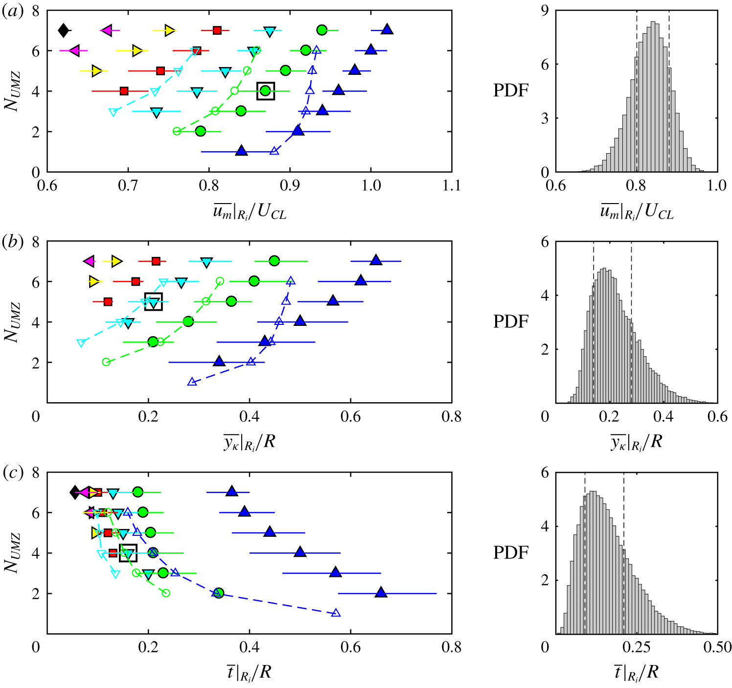
Figure 5. Conditional averages of UMZ groups  $R_{i}$ based on the zone rank of zone modal velocity
  $u_{m}$ for different
  $N_{UMZ}$: (a) zone modal velocity,
  $u_{m}|_{R_{i}}$, (b) zone distance from wall,
  $1-r_{\unicode[STIX]{x1D705}}|_{R_{i}}$ and (c) zone thickness,
  $t|_{R_{i}}$. The bars are the span of the centred 50 % of the data and the filled marker on each bar indicates the mean. The hollowed markers with dashed lines are results from a turbulent boundary layer by Laskari et al. (Reference Laskari, de Kat, Hearst and Ganapathisubramani2018). The same symbols represent the same ranks in a pipe (filled) and TBL (hollowed). (Symbols and colours as in table 1 (left).) The PDFs on the right-hand side are shown for one rank group at a certain
  $N_{UMZ}$ with its marker boxed in the left-hand side figures. The two dashed lines on the PDFs indicate the centred 50 % (25 % to 75 %) of the data.
In figure 5(a), when  $N_{UMZ}=1$, only group
  $R_{1}$ (marked by ‘
 $u_{m}$ in each snapshot is present. As
  $N_{UMZ}$ increases, more zones in lower ranking groups become available. The trend of
  $u_{m}$ with increasing
  $N_{UMZ}$ is very clear and similar for all existing zones: all the existing zones have increased
  $u_{m}$ while the newly joined zone in a lower rank (
 $R_{i}$ with
  $i=N_{UMZ}$) starts at the lowest
  $u_{m}$ at that
  $N_{UMZ}$. As
  $N_{UMZ}$ continues to increase, the recently joined zones exhibit similar increase in
  $u_{m}$ and the UMZs in the newest/lowest rank start at an even lower
  $u_{m}$. This forms a triangular-shape distribution of
  $u_{m}$ along
  $N_{UMZ}$ in figure 5(a). Figure 5(b) shows the average wall-normal location of the UMZs in group
  $R_{1:6}$,
  $y_{\unicode[STIX]{x1D705}}$. The wall-normal location of each UMZ is defined as the distance between the wall and the lower UMZ interface closer to the wall which bounds the UMZ and its adjacent zone with lower
  $u_{m}$ (see figure 2c). The distribution and the trend of
  $y_{\unicode[STIX]{x1D705}}$ is very similar to
  $u_{m}$ along
  $N_{UMZ}$. All the existing zones move towards the centre of the pipe when the new zones join near the wall with lower
  $y_{\unicode[STIX]{x1D705}}$. This matches the observation by Laskari et al. (Reference Laskari, de Kat, Hearst and Ganapathisubramani2018) that when more zones are in presence, the zones are, on average, pushed to the centre to accommodate more UMZs in the region. This would result in all UMZs being thinner on average at higher
  $N_{UMZ}$ which is shown in figure 5(c). When
  $N_{UMZ}$ increases, the zone modal velocity
  $u_{m}$ and wall distance
  $y_{\unicode[STIX]{x1D705}}$ of the UMZs in each rank all increase with zone thickness
  $t$ decreasing monotonically. This suggests that the UMZs are thinner and travelling faster when there are more UMZs in the flow region.
 The TBL results from Laskari et al. (Reference Laskari, de Kat, Hearst and Ganapathisubramani2018) for the first three ranking groups  $R_{1:3}$ are overlaid on the left-hand side distributions in figure 5. The same symbol is used for the same ranking group in the pipe (colour filled) and TBL (hollowed with a dashed line along each rank). The trend of monotonically increasing
  $u_{m}$ and
  $y_{\unicode[STIX]{x1D705}}$ and decreasing
  $t$ is very similar between pipe and TBL, especially for ranks
  $R_{2}$ and lower. However, the
  $R_{1}$ zones show marked differences between pipe (‘
 $R_{1}$ UMZs in TBL increases with
  $N_{UMZ}$ more slowly than the other ranks whereas the
  $R_{1}$ zone in the pipe is similar to all the other ranks and
  $R_{2,3}$ of the TBL with a continuous increase in
  $u_{m}$ all the way along
  $N_{UMZ}$. At
  $N_{UMZ}=1$, the
  $R_{1}$ zones in TBL start at a
  $u_{m}$ 5 % higher than a pipe whereas at
  $N_{UMZ}=6$, the
  $R_{1}$ zones in a pipe with faster increase than the TBL have
  $u_{m}$ 14 % higher than the TBL. In a TBL, the maximum
  $u_{m}$ reached by
  $R_{1}$ is approximately
  $0.93U_{\infty }$ whereas in a pipe, the
  $R_{1}$ zones can reach beyond the pipe centreline velocity at
  $u_{m}/U_{CL}\approx 1.02$. A similar slower increase in wall distance
  $y_{\unicode[STIX]{x1D705}}$ of
  $R_{1}$ in a TBL compared to its other two ranks
  $R_{2,3}$ and all the ranks in a pipe is shown in figure 5(b). The most significant difference between the pipe and TBL is in the zonal thickness
  $t$ in figure 5(c). The
  $R_{1}$ zones in a pipe are significantly thicker than the lower ranks, whereas the
  $R_{1}$ zones in the TBL did not show such a step change between
  $\unicode[STIX]{x0394}t|_{R_{1,2}}$ and
  $\unicode[STIX]{x0394}t|_{R_{2,3}}$. The
  $R_{1}$ zones correspond to the innermost zones in the pipe and the zones closest to the free stream in the TBL. The distribution of
  $u_{m}$,
  $y_{\unicode[STIX]{x1D705}}$ and
  $t$ for all ranks in the TBL is generally similar to a pipe for rank
  $R_{2}$ and below. This most centred UMZ is often referred to as the quiescent core of the pipe (and the channel) which can travel faster than the centreline velocity whereas in the TBL, all UMZs below the TNTI travel at velocities lower than the free-stream velocity. The significant differences observed in the
  $R_{1}$ zones of the pipe and TBL indicate that the first UMZ below the TNTI in a TBL does not correspond to the innermost zone in the pipe. Given the close similarity between the pipe and channel (Kwon et al. Reference Kwon, Philip, de Silva, Hutchins and Monty2014; Kwon Reference Kwon2016; Yang et al. Reference Yang, Hwang and Sung2016), figure 5 suggests that the innermost UMZ in the pressure-driven wall turbulent flows behaves differently from the
  $R_{1}$ UMZ in the shear-driven TBL.
3.3 Characterisation of UMZ and UMZ interface
3.3.1 Wall-normal location of UMZ
The wall-normal location of the UMZs  $y_{\unicode[STIX]{x1D705}}$ is averaged for UMZs in each group of the two grouping methods. Figure 6(a) shows
  $\langle y_{\unicode[STIX]{x1D705}}\rangle$ for
  $u_{m}$ groups
  $M_{1:6}$. The angle brackets
  $\langle \rangle$ indicate conditional average for UMZs in each group. The UMZs in group
  $M_{6}$ with the lowest
  $u_{m}/U_{CL}\in [0.5,0.6)$ are very close to the wall with
  $\langle y_{\unicode[STIX]{x1D705}}\rangle$ almost equal to zero;
  $y_{\unicode[STIX]{x1D705}}$ gradually increases from
  $M_{6}$ to
  $M_{1}$ which has
  $\langle y_{\unicode[STIX]{x1D705}}\rangle /R\approx 0.75$. The trend follows the mean profile of
  $U$ plotted as
  $y(\overline{U})$ (dashed line). The change in
  $y_{\unicode[STIX]{x1D705}}$ is rather small near the wall for groups
  $M_{6:4}$ and becomes large for
  $M_{3:1}$ towards the pipe centre. In figure 6(b) for
  $\langle y_{\unicode[STIX]{x1D705}}\rangle$ of UMZs in each ranking group
  $R_{1:7}$, a similar trend is shown. The nonlinear increase of
  $y_{\unicode[STIX]{x1D705}}$ from
  $R_{7}$ to
  $R_{1}$ indicates that the UMZs at lower ranks are more closely distributed nearer the wall while the higher ranked UMZs (
 $R_{1:3}$) are thicker so that they are further apart from each other towards the pipe centre. The results of
  $y_{\unicode[STIX]{x1D705}}$ using both grouping methods indicate that the UMZs are not uniformly distributed from the centreline to the wall but in a hierarchical distribution where zones near the wall are more densely populated, similar to TBL (de Silva et al. Reference de Silva, Hutchins and Marusic2016, Reference de Silva, Philip, Hutchins and Marusic2017).
The average thickness of the UMZs in each group can be calculated from the radial location  $r_{\unicode[STIX]{x1D705}}$ of the zones. The calculation is illustrated in figure 7(a) for the grouping method based on the ranking of
  $u_{m}$. The illustration is idealised to have three UMZs ranked from
  $R_{1}$ to
  $R_{3}$. Note that the thickness of the innermost zone equals its radial location
  $r_{\unicode[STIX]{x1D705}}$. Figure 7(b) shows the group average thickness
  $\langle t\rangle$ of the UMZs calculated from
  $1-\langle y_{\unicode[STIX]{x1D705}}\rangle$. The value of
  $\langle t\rangle$ from group
  $R_{7}$ to
  $R_{1}$ increases monotonically: UMZs are the thinnest nearer the wall and the zone thickness increases when departing from the wall. The slope of
  $\langle t\rangle$ decreases group by group from the wall (
 $R_{7}$) toward the pipe centre until the second innermost group (
 $R_{2}$), then there is a sudden increase in the slope of
  $\langle t\rangle$ for the innermost zones (
 $R_{1}$ and
  $M_{1}$). This supports the previous finding in § 3.2 where the innermost UMZs in the pipe flow were found to be much thicker than the other UMZs in a pipe and the UMZ below the TNTI in a TBL. This is understood as in a pipe and channel, the opposing walls each have a flow similar to a TBL so that the innermost zone in a pipe contains the zones furthest away from the opposing walls interacting at the centre.

Figure 6. Conditionally averaged zone interface wall-normal location  $y_{\unicode[STIX]{x1D705}}=1-r_{\unicode[STIX]{x1D705}}$ (
 $r_{\unicode[STIX]{x1D705}}$ is the radial location) for UMZs grouped by (a) zone modal velocity
  $u_{m}$,
  $u_{m}$ groups
  $M_{1:6}$ and (b) by zone rank of
  $u_{m}$, ranking groups
  $R_{1:7}$. The dashed line in (a) is the mean velocity profile of
  $\overline{U}$ plotted as
  $y(\overline{U})$.

Figure 7. (a) An illustration of computing the average UMZ thickness of each  $u_{m}$ and ranking group,
  $\langle t\rangle$ from the average UMZ radial location
  $r_{\unicode[STIX]{x1D705}}$ of each group. (b) The average UMZ thickness
  $\langle t\rangle$ of each ranking group
  $R_{i}$.
3.3.2 Zonal means inside and outside the UMZs
In order to investigate how UMZs at different wall-normal locations differ from each other, the zonal mean statistics of the UMZs in different  $u_{m}$ groups
  $M_{1:5}$ are computed. The zonal mean inside a UMZ is averaged in the region between the UMZ lower-bounding interface closer to the wall up to the centreline, in other words, over its radial extent from the pipe centre (see the definition of
  $r_{\unicode[STIX]{x1D705}}$ in figure 2c); the zonal mean outside a UMZ is averaged over the region outside its lower bounding interface at
  $r_{\unicode[STIX]{x1D705}}$ towards the wall. Means inside the UMZ are denoted with a hat as
  $\widehat{U}$ and
  $\widehat{u^{2}}$; means outside the UMZ are denoted with a tilde as
  $\widetilde{U}$ and
  $\widetilde{u^{2}}$, similar to Kwon et al. (Reference Kwon, Philip, de Silva, Hutchins and Monty2014). Figure 8 shows the zonal mean inside (
 $\widehat{U}$,
  $\widehat{u^{2}}$) with dot-dashed lines and zonal means outside (
 $\widetilde{U}$,
  $\widetilde{u^{2}}$) with dashed lines. The global average profiles of
  $\overline{U}$ and
  $\overline{u^{2}}$ with solid lines are shown as references.
In figure 8(a), the zonal mean profiles  $U$ are plotted for
  $u_{m}$ groups
  $M_{1:5}$. The mean streamwise velocity inside the UMZ (
 $\widehat{U}$) is always larger than the time mean (
 $\overline{U}$) whereas the mean outside the UMZ (
 $\widetilde{U}$) is always smaller than
  $\overline{U}$. The velocity difference between
  $\widehat{U}$ and
  $\widetilde{U}$ for each
  $u_{m}$ group
  $M_{i}$ indicates the velocity jump across the UMZ interface (see figure 9). The value of
  $\widetilde{U}$ for each
  $u_{m}$ group follows the time mean
  $\overline{U}$ profile very near the wall and starts to deviate from
  $\overline{U}$ away from the wall. The
  $\widehat{U}$ data are available in a large range of wall-normal locations, and can extend very close to the wall at
  $y/R\approx 0.01$ for group
  $M_{5}$. This shows the large meandering behaviour of the UMZ. To measure the level of meandering of the UMZs in terms of how far they can extend towards the wall in extreme cases, figure 8(b) shows the minimum wall-normal location
  $\widehat{y}$ that the UMZ can extend to (where
  $\widehat{U}$ is last available near the wall). The value of
  $\widehat{y}$ for group
  $M_{5:2}$ increases steadily from the wall to the centre from
  $\widehat{y}/R\approx 0.01$ to
  $0.05$ whereas the innermost UMZs with
  $u_{m}>U_{CL}$ in group
  $M_{1}$ can extend significantly less close to the wall with
  $\widehat{y}/R\approx 0.22$.
Figure 8(c,d) shows the zonal mean profiles of  $U$ and
  $u^{2}$ for UMZs in group
  $M_{2}$ only. This provides a relatively direct comparison between a pipe and channel: UMZs in group
  $M_{2}$ have
  $u_{m}/Ucl\in [0.9,1)$ and the channel results are from a single UMZ defined at a fixed
  $u_{\unicode[STIX]{x1D705}}/U_{CL}=0.95$. In figure 8(c), the pipe profiles of group
  $M_{2}$ can extend further towards the wall due to the grouping: some of the UMZs in group
  $M_{2}$ are defined at a lower threshold velocity
  $u_{\unicode[STIX]{x1D705}}$ than the channel core so that they are naturally thicker and closer to the wall. The differences between the pipe profiles (in red) and the channel profiles (in black) are mainly caused by the difference in
  $\overline{U}$ due to the Reynolds number difference. Higher Reynolds number of the channel (
 $Re_{\unicode[STIX]{x1D70F}}=1000$) has
  $\overline{U}$ developing faster nearer the wall. Otherwise, the trend between
  $\widehat{U}$,
  $\widetilde{U}$ and
  $\overline{U}$ is very similar in a pipe and channel. In figure 8(d), the zonal mean streamwise fluctuation
  $u^{2}$ is computed relative to zonal means of
  $U$ following Kwon et al. (Reference Kwon, Philip, de Silva, Hutchins and Monty2014)
 $$\begin{eqnarray}\widehat{u^{2}}=(U-\widehat{U})^{2},\quad \widetilde{u^{2}}=(U-\widetilde{U})^{2}.\end{eqnarray}$$
 The turbulent intensity inside the UMZ,  $\widehat{u^{2}}$, is much lower than the turbulent intensity outside the zone,
  $\widetilde{u^{2}}$. The difference between
  $\widehat{u^{2}}$ and
  $\widetilde{u^{2}}$ becomes smaller towards the centreline;
  $\widehat{u^{2}}$ and
  $\widetilde{u^{2}}$ cross over at
  $y/R\approx 0.74$ where
  $\widehat{u^{2}}$ starts to be larger than
  $\widetilde{u^{2}}$ until the centreline (see zoomed view inside figure 8d). A similar behaviour of
  $\widehat{u^{2}}$ and
  $\widetilde{u^{2}}$ was observed in the channel (Kwon et al. Reference Kwon, Philip, de Silva, Hutchins and Monty2014) and the cross-over point of
  $\widetilde{u^{2}}>\widehat{u^{2}}$ was also at
  $y/h\approx 0.74$ (
 $h$ is the channel half-height). Therefore, despite the Reynolds number effect, the quiescent core of channel and the UMZs (
 $M_{2}$) of a pipe are very similar.

Figure 8. Zonal mean profiles of the streamwise velocity  $U$ for UMZs in
  $u_{m}$ groups (a)
  $M_{1:5}$ with colours as in table 1 and (c)
  $M_{2}$ (in red) overlaid with channel flow results by Kwon et al. (Reference Kwon, Philip, de Silva, Hutchins and Monty2014) (in black). (b) The wall-normal location of the most near-wall data of the zonal mean inside the UMZs of each group in (a),
  $\widehat{y}$ (symbols as in table 1). (d) The streamwise velocity fluctuation
  $u^{2}$ for group
  $M_{2}$ only. The solid lines (——) are the time averages of
  $U$ and
  $u^{2}$ in (a,c,d). The dot-dashed lines (— ⋅ —) are the zonal means inside the UMZ,
  $\widehat{U}$ and
  $\widehat{u^{2}}$; the dashed lines (- - - -) are the zonal means outside the UMZ,
  $\widetilde{U}$ and
  $\widetilde{u^{2}}$.

Figure 9. Conditional averages as functions of the distance from the lower-bounding UMZ interface ( $\unicode[STIX]{x1D709}$) for (a) the streamwise velocity
  $U$ for
  $u_{m}$ group
  $M_{2}$, (b)
  $U$ for groups
  $M_{1:4}$, (c) velocity gradient
  $\unicode[STIX]{x2202}U/\unicode[STIX]{x2202}\unicode[STIX]{x1D709}$ for group
  $M_{2}$, (d)
  $\unicode[STIX]{x2202}U/\unicode[STIX]{x2202}\unicode[STIX]{x1D709}$ for groups
  $M_{1:4}$, (e) streamwise velocity fluctuation
  $u^{\ast 2}$ for group
  $M_{2}$ and (f)
  $u^{\ast 2}$ for groups
  $M_{1:4}$. The legends in (e) and (f) apply to (a,c) and (b,d) respectively. (g) The magnitude of velocity jump in
  $U$ across the UMZ interface,
  $\unicode[STIX]{x0394}U$ for groups
  $M_{1:4}$. (h) The UMZ interface thickness
  $\unicode[STIX]{x1D6FF}_{\unicode[STIX]{x1D714}}$ calculated from (3.1) for groups
  $M_{1:4}$. (g,h) Are overlaid with TBL results by de Silva et al. (Reference de Silva, Philip, Hutchins and Marusic2017) at
  $Re_{\unicode[STIX]{x1D70F}}=14\,500$ (
 $\times$),
  $Re_{\unicode[STIX]{x1D70F}}=8000$ (○),
  $Re_{\unicode[STIX]{x1D70F}}=2800$ (
 $+$) and
  $Re_{\unicode[STIX]{x1D70F}}=1200$ (▵).
3.3.3 Conditional average across the UMZ interface
Conditional averages are computed for flow properties across the UMZ interface as functions of the distance from the interface,  $\unicode[STIX]{x1D709}$. Figure 9(a) shows the group average streamwise velocity
  $\langle U\rangle$ against
  $\unicode[STIX]{x1D709}$ for a single
  $u_{m}$ group
  $M_{2}$, overlaid with results from the channel (Yang et al. Reference Yang, Hwang and Sung2016). The angle brackets
  $\langle \rangle$ in this section indicate conditional averaging across the interface for UMZs in each
  $u_{m}$ group;
  $\unicode[STIX]{x1D709}=0$ indicates the UMZ interface and
  $\unicode[STIX]{x1D709}>0$ represents the inside of the UMZ. In figure 9(a), the abrupt jumps in
  $U$ across the interface are similar between UMZs in
  $M_{2}$ and the quiescent core of the channel: before entering the zone (
 $\unicode[STIX]{x1D709}<0$),
  $U$ develops fairly slowly until the near vicinity of the interface where it experiences a sharp change of the rate. The velocity gradient
  $\unicode[STIX]{x2202}U/\unicode[STIX]{x2202}\unicode[STIX]{x1D709}$ of group
  $M_{2}$ is shown in figure 9(c), overlaid with the results of the quiescent cores in the channel (Kwon et al. Reference Kwon, Philip, de Silva, Hutchins and Monty2014; Yang et al. Reference Yang, Hwang and Sung2016). A local maximum of velocity gradient corresponding to the abrupt jump in
  $U$ at the interface is similar here in a pipe. The streamwise fluctuation
  $u^{2}$ across the UMZ interface is shown in figure 9(e,f). In figure 9(e), for UMZs in group
  $M_{2}$ of pipe and the quiescent core of channel,
  $u^{2}$ behaves very similarly in a pipe and channel in which the streamwise fluctuation decreases dramatically across the interface with a local minimum at
  $\unicode[STIX]{x1D709}\approx 0$, and then remains very low inside the UMZ. In figure 9(f), the
  $u^{2}$ profiles for groups
  $M_{3,4}$ are different from groups
  $M_{1,2}$ because the UMZs in groups
  $M_{3,4}$ travelling at lower
  $u_{m}$ are very close to the wall, close enough to capture the rapid increase in
  $\overline{u^{2}}$ in the near-wall region (see figure 8d for
  $y/R<0.05$).
Figure 9(b) shows  $\langle U\rangle$ against
  $\unicode[STIX]{x1D709}$ for
  $u_{m}$ groups
  $M_{1:4}$. The increase in
  $U$ across the UMZ interface is larger (higher magnitude) and more abrupt (higher velocity gradient) for interfaces closer to the wall, as found in TBL (de Silva et al. Reference de Silva, Philip, Hutchins and Marusic2017). Figure 9(d) corresponds to figure 9(b), showing the increase in maximum velocity gradient at
  $\unicode[STIX]{x1D709}=0$ for UMZs nearer the wall travelling at lower
  $u_{m}$. The magnitude of the velocity jump,
  $\unicode[STIX]{x0394}U$ is defined similar to Yang et al. (Reference Yang, Hwang and Sung2016), as illustrated in figure 9(a). The value of
  $\unicode[STIX]{x0394}U$ for UMZs in group
  $M_{1:4}$ is shown in figure 9(g) with the TBL results (de Silva et al. Reference de Silva, Philip, Hutchins and Marusic2017) at
  $Re_{\unicode[STIX]{x1D70F}}=8000$ and
  $14\,500$. The values of
  $\unicode[STIX]{x0394}U$ in both pipe and TBL are found to be larger for UMZs travelling at lower
  $u_{m}$ nearer the wall. The overall magnitude of
  $\unicode[STIX]{x0394}U$ in the pipe is significantly larger than the TBL. This is partly caused by the lower Reynolds number in the pipe: the number of UMZs is generally lower at lower Reynolds number so that
  $U$ jumps across fewer interfaces with larger
  $\unicode[STIX]{x0394}U$ to achieve the centreline velocity. This increase in
  $\unicode[STIX]{x0394}U$ with decreasing Reynolds number is shown by the TBL results where the
  $Re_{\unicode[STIX]{x1D70F}}=8000$ case (‘○’) has higher
  $\unicode[STIX]{x0394}U$ than
  $Re_{\unicode[STIX]{x1D70F}}=14\,500$ (‘
 $\times$’). However, the increase in
  $\unicode[STIX]{x0394}U$ with lowering Reynolds number is not as significant as the difference in
  $\unicode[STIX]{x0394}U$ between the pipe and TBL. This suggest that the velocity jump of
  $U$ across the UMZ interface is, on average, stronger in a pipe than TBL.
In figure 9(a–d), the velocity jumps and the peaked velocity gradients at the UMZ interface take place in a narrow distance over  $\unicode[STIX]{x1D709}$ as the UMZ interfaces themselves have a thickness (de Silva et al. Reference de Silva, Philip, Hutchins and Marusic2017). The thickness of the interfaces is estimated by
 $$\begin{eqnarray}\unicode[STIX]{x1D6FF}_{\unicode[STIX]{x1D714}}=\frac{\unicode[STIX]{x0394}\langle U\rangle }{\unicode[STIX]{x2202}\langle U\rangle /\unicode[STIX]{x2202}y|_{max}},\end{eqnarray}$$
 following Kwon et al. (Reference Kwon, Philip, de Silva, Hutchins and Monty2014) and de Silva et al. (Reference de Silva, Philip, Hutchins and Marusic2017). Figure 9(h) shows the UMZ interface thickness  $\unicode[STIX]{x1D6FF}_{\unicode[STIX]{x1D714}}$ for groups
  $M_{1:4}$. The value of
  $\unicode[STIX]{x1D6FF}_{\unicode[STIX]{x1D714}}$ is lower for UMZs closer to the wall as found in the TBL, so that the thinner UMZs nearer the wall also have thinner interfaces accompanied by a sharper and larger jump in
  $U$. The hierarchical distribution of the UMZ and UMZ interface and the magnitude of
  $\unicode[STIX]{x0394}U$ together suggest a discrete step-like model of the velocity profile in wall turbulence which has been used as the initial velocity profile in the turbulence modelling by Bautista et al. (Reference Bautista, Ebadi, White, Chini and Klewicki2019). The overlaid TBL results of
  $\unicode[STIX]{x1D6FF}_{\unicode[STIX]{x1D714}}$ at
  $Re_{\unicode[STIX]{x1D70F}}=1200{-}14\,500$ are roughly in the range of
  $u_{m}$ in group
  $M_{3}$ of the pipe. The interface thickness in the TBL increases when
  $Re_{\unicode[STIX]{x1D70F}}$ decreases, as expected, since there are less UMZs at larger scales at lower Reynolds number. The UMZ interface in a pipe at a much lower
  $Re_{\unicode[STIX]{x1D70F}}=500$ has
  $\unicode[STIX]{x1D6FF}_{\unicode[STIX]{x1D714}}$ in between the
  $Re_{\unicode[STIX]{x1D70F}}=2800$ and
  $1200$ cases of the TBL, indicating that the UMZ interfaces are, on average, thinner in a pipe than TBL. This supports the previous finding where the velocity jump in
  $U$ was found to be stronger in a pipe so that the velocity jumps in a pipe are more abrupt over thinner interfaces in a pipe than TBL. That the UMZ interfaces are found to be thinner in the DNS data of a pipe than the experimental data of a TBL may also be due to the limited spatial resolution in the experiments.
Figure 10(a) shows the conditional average of azimuthal vorticity  $\langle \unicode[STIX]{x1D6FA}_{\unicode[STIX]{x1D703}}\rangle$ against
  $\unicode[STIX]{x1D709}$ where
  $\unicode[STIX]{x1D6FA}_{\unicode[STIX]{x1D703}}=\unicode[STIX]{x2202}V_{r}/\unicode[STIX]{x2202}x-\unicode[STIX]{x2202}U/\unicode[STIX]{x2202}r$;
  $\unicode[STIX]{x1D6FA}_{\unicode[STIX]{x1D703}}$ peaks in the proximity of the interface similar to
  $\unicode[STIX]{x2202}U/\unicode[STIX]{x2202}\unicode[STIX]{x1D709}$ in figure 9(d). The initial
  $\unicode[STIX]{x1D6FA}_{\unicode[STIX]{x1D703}}$ away from the interface at
  $\unicode[STIX]{x1D709}/R=-0.2$ is significantly higher for UMZ groups closer to the wall since vorticities are stronger nearer the wall. The local maximum of
  $\unicode[STIX]{x1D6FA}_{\unicode[STIX]{x1D703}}$ at
  $\unicode[STIX]{x1D709}=0$ in figure 10(a) and
  $\unicode[STIX]{x2202}U/\unicode[STIX]{x2202}\unicode[STIX]{x1D709}$ in figure 9(d) are plotted in figure 10(b). The peak azimuthal vorticity and streamwise velocity gradient have very similar trends:
  $\unicode[STIX]{x1D6FA}_{\unicode[STIX]{x1D703}}$ and
  $\unicode[STIX]{x2202}U/\unicode[STIX]{x2202}\unicode[STIX]{x1D709}$ both decrease almost log-linearly from the wall (
 $M_{4}$) towards the centre (
 $M_{2}$), apart from the innermost UMZs in group
  $M_{1}$, which shows a lowered rate of decrease. The differences in conditional averages of the innermost UMZs from the other zones are consistent with the findings in the previous §§ 3.3.1 and 3.2.

Figure 10. (a) Conditional-average azimuthal vorticity  $\unicode[STIX]{x1D6FA}_{\unicode[STIX]{x1D703}}$ for
  $u_{m}$ groups
  $M_{1:4}$ as a function of the distance from the lower-bounding UMZ interface. (b) The local maximum
  $\unicode[STIX]{x1D6FA}_{\unicode[STIX]{x1D703}}$ (in a) and
  $\unicode[STIX]{x2202}U/\unicode[STIX]{x2202}\unicode[STIX]{x1D709}$ (in figure 8d) at the UMZ interface (
 $\unicode[STIX]{x1D709}\approx 0$).
3.4 The vortex–interface attachment
3.4.1 Dynamics of the attachment
The local maximum azimuthal vorticity  $\unicode[STIX]{x1D6FA}_{\unicode[STIX]{x1D703}}$ at the UMZ interface in figure 10(a) suggests a strong correlation between the UMZ interfaces and the vortical structures. Figure 11 shows an instantaneous UMZ interface defined at
  $u_{\unicode[STIX]{x1D705}}/U_{CL}=0.8$ in (a) and
  $0.9$ in (b) for the same snapshot in the streamwise plane, superpositioned on the contour of
  $\unicode[STIX]{x1D6FA}_{\unicode[STIX]{x1D703}}$ (with the prograde vortices in red and the retrograde vortices in blue). Different colour scales are used in figure 11(a,b) to improve the clarity of the contours of the surrounding vortical structures at different strengths. On these streamwise planes, the interface continuously follows the azimuthal vortices with similar strength, so that the
  $u_{\unicode[STIX]{x1D705}}/U_{CL}=0.8$ interface in figure 11(a) is generally much closer to the wall, being attached to stronger vortices nearer the wall. This is consistent with the observations by Adrian et al. (Reference Adrian, Meinhart and Tompkins2000) where patches of spanwise vortices were found aligned along the strong shear layers inside a TBL. In figure 11, the UMZ interface threads through the azimuthal vortices and folds into bulges and valleys to form a persistent vortex–interface attachment.
The dynamics of this vortex–interface attachment is further investigated. Supplementary movies of the attachment between vortices and UMZ interfaces over time are available in both fixed and moving frames at https://doi.org/10.1017/jfm.2019.947 (movies 1–4). Figure 12 shows three snapshots from the moving-frame video with a constant time gap. In these snapshots, the interface contorts to follow the inclined trains of eddies (marked with dashed lines) from the wall towards the pipe centre. The interface initially attached to vortex  $A$ in figure 12(a) meanders as vortex
  $A$ deforms and moves with the flow in figure 12(b). In figure 12(c), when vortex A is weakened and merged with weaker eddies, the local interface changes significantly to reattach to a nearby vortex at
  $A^{\prime }$ to maintain the desirable vortical strength. The weakened vortex
  $A$ then attaches to an iso-surface defined at a lower velocity threshold.

Figure 11. Contours of azimuthal vorticity  $\unicode[STIX]{x1D6FA}_{\unicode[STIX]{x1D703}}$ in the streamwise plane, super-positioned with instantaneous UMZ interfaces defined at (a)
  $u_{\unicode[STIX]{x1D705}}/U_{CL}=0.8$ and (b)
  $u_{\unicode[STIX]{x1D705}}/U_{CL}=0.9$ for the same snapshot. The background contours of
  $\unicode[STIX]{x1D6FA}_{\unicode[STIX]{x1D703}}$ in (a,b) only differ in the colour axis.

Figure 12. Contours of  $\unicode[STIX]{x1D6FA}_{\unicode[STIX]{x1D703}}$ and the UMZ interface defined at
  $u_{\unicode[STIX]{x1D705}}/U_{CL}=0.9$ plotted on a streamwise moving frame approximately at the flow speed downstream with time from (a) to (c) with a uniform time gap between each two of the three snapshots. Label
  $A$ in (a,b) marks a prograde vortex weakened and joined the nearby vortices at
  $A^{\prime }$ in (c). Label
  $B$ marks a strong retrograde vortex the interface is attached to. (The arrows show the vector of streamwise and wall-normal velocity fluctuations,
  $u$ and
  $v$.)
$v$.)

Figure 13. (a) Contour of azimuthal vorticity  $\unicode[STIX]{x1D6FA}_{\unicode[STIX]{x1D703}}$ in a cross-stream plane, superpositioned with an instantaneous UMZ interface defined at
  $u_{\unicode[STIX]{x1D705}}/U_{CL}=0.9$. (b) A 3-D instantaneous UMZ interface defined at
  $u_{\unicode[STIX]{x1D705}}/U_{CL}=0.8$ with colour based on the azimuthal vorticity
  $\unicode[STIX]{x1D6FA}_{\unicode[STIX]{x1D703}}$ on the interface surface. The UMZ interface is shown for
  $1/6$ of the streamwise extent, unwrapped in the azimuthal direction.
3.4.2 The three-dimensional attachment
Figure 13(a) shows the vortex–interface attachment in the azimuthal direction of the pipe on a cross-stream plane for a UMZ interface defined at  $u_{\unicode[STIX]{x1D705}}/U_{CL}=0.8$ corresponding to figure 11(b). The azimuthal vortices have elongated tube shapes in the azimuthal direction and vortices at similar strengths vary in their wall distance. Similar to the attachment shown in the streamwise direction in figure 11 and also Adrian et al. (Reference Adrian, Meinhart and Tompkins2000), the UMZ interface contorts to attach to individual vortices and switches at the gaps between the azimuthal vortices to attach to the next vortex at desired strength. The 3-D attachment for the UMZ interface is shown in figure 13(b) for a UMZ interface defined at
  $u_{\unicode[STIX]{x1D705}}/U_{CL}=0.8$. The attachment of the UMZ interface to vortical structures is significantly biased to the prograde vortices (in red) whereas the retrograde vortices (blue) are rarely found on the interface surface. To quantify the attachment, figure 14(a) shows the time-average PDFs of
  $\unicode[STIX]{x1D6FA}_{\unicode[STIX]{x1D703}}$ on the 3-D interface surface of the UMZs in
  $u_{m}$ groups
  $M_{1:4}$. Through group
  $M_{1}$ to
  $M_{5}$ from the centre to the wall, there is a continuous increase in the skewness of prograde vortices (defined as positive
  $\unicode[STIX]{x1D6FA}_{\unicode[STIX]{x1D703}}$) denoted as
  $\unicode[STIX]{x1D6FA}_{\unicode[STIX]{x1D703}}^{p}$, which is the strongest closest to the wall. The negative ends of the PDFs representing attachment on retrograde vortices (
 $\unicode[STIX]{x1D6FA}_{\unicode[STIX]{x1D703}}^{r}$) show small changes for different UMZ groups. The magnitude of prograde vorticity
  $\unicode[STIX]{x1D6FA}_{\unicode[STIX]{x1D703}}^{p}$ at a fixed PDF of
  $10^{-4}$ for each
  $u_{m}$ group (marked by ‘
 $\times$’ along the dashed line at PDF
 $=10^{-4}$) is shown in figure 14(b). The increase in
  $\unicode[STIX]{x1D6FA}_{\unicode[STIX]{x1D703}}^{p}$ against UMZ modal velocity
  $u_{m}$ shows a marked linearity, even for the fastest travelling UMZs in group
  $M_{1}$ which have been found to be different from the other groups in the previous results. The linear increase of
  $\unicode[STIX]{x1D6FA}_{\unicode[STIX]{x1D703}}^{p}$ towards the wall against
  $u_{m}$ has a slope of
  $\text{d}\unicode[STIX]{x1D6FA}_{\unicode[STIX]{x1D703}}^{p}/\text{d}u_{m}\approx 66.4$ with negligible variation (maximum 4.8 %) between different
  $u_{m}$ groups.

Figure 14. (a) PDF of the azimuthal vorticity  $\unicode[STIX]{x1D6FA}_{\unicode[STIX]{x1D703}}$ on the 3-D UMZ interfaces for
  $u_{m}$ groups
  $M_{i=1:5}$. Here,
  $\unicode[STIX]{x1D6FA}_{\unicode[STIX]{x1D703}}$ is defined as positive for prograde vortices and negative for retrograde vortices. (b) The magnitude of positive prograde azimuthal vorticity,
  $\unicode[STIX]{x1D6FA}_{\unicode[STIX]{x1D703}}^{p}$ at a probability density of
  $10^{-4}$ for groups
  $M_{1:5}$ (marked by ‘
 $\times$’ in (a)).

Figure 15. Conditional-average profiles of total azimuthal vorticity  $\unicode[STIX]{x1D6FA}_{\unicode[STIX]{x1D703}}$, prograde vorticity
  $\unicode[STIX]{x1D6FA}_{\unicode[STIX]{x1D703}}^{p}$ and retrograde vorticity
  $\unicode[STIX]{x1D6FA}_{\unicode[STIX]{x1D703}}^{r}$ as functions of distance from the UMZ interface (
 $\unicode[STIX]{x1D709}$) for
  $u_{m}$ group
  $M_{2}$. The total azimuthal vorticity
  $\unicode[STIX]{x1D6FA}_{\unicode[STIX]{x1D703}}=\unicode[STIX]{x1D6FA}_{\unicode[STIX]{x1D703}}^{p}-\unicode[STIX]{x1D6FA}_{\unicode[STIX]{x1D703}}^{r}$. The inset shows the ratio between the prograde and retrograde vorticity
  $\unicode[STIX]{x1D6FA}_{\unicode[STIX]{x1D703}}^{p}/\unicode[STIX]{x1D6FA}_{\unicode[STIX]{x1D703}}^{r}$ against
  $\unicode[STIX]{x1D709}$.
Figure 15 shows the conditional-average vorticity of the prograde ( $\unicode[STIX]{x1D6FA}_{\unicode[STIX]{x1D703}}^{p}$) and retrograde (
 $\unicode[STIX]{x1D6FA}_{\unicode[STIX]{x1D703}}^{r}$) vortices for UMZs in group
  $M_{2}$ against
  $\unicode[STIX]{x1D709}$. At the interface (
 $\unicode[STIX]{x1D709}=0$) where the total
  $\unicode[STIX]{x1D6FA}_{\unicode[STIX]{x1D703}}$ peaks in figure 10, here, it shows that nearly all
  $\unicode[STIX]{x1D6FA}_{\unicode[STIX]{x1D703}}$ is contributed from
  $\unicode[STIX]{x1D6FA}_{\unicode[STIX]{x1D703}}^{p}$ while
  $\unicode[STIX]{x1D6FA}_{\unicode[STIX]{x1D703}}^{r}$ decreases to a local minimum at the UMZ interface. The distribution of
  $\unicode[STIX]{x1D6FA}_{\unicode[STIX]{x1D703}}^{p,r}$ for group
  $M_{2}$ is, again, very similar to the quiescent core in the channel (Yang et al. Reference Yang, Hwang and Sung2016). Inside figure 15, the ratio of prograde and retrograde vorticity peaks at the interface, achieving
  $\unicode[STIX]{x1D6FA}_{\unicode[STIX]{x1D703}}^{p}/\unicode[STIX]{x1D6FA}_{\unicode[STIX]{x1D703}}^{r}\approx 25$ for UMZs in group
  $M_{2}$. Results in this section suggest that the contorted shape of the UMZ interface is a consequence of its attachment to the azimuthal/spanwise vortices which move three-dimensionally with varying wall-normal location. Additionally, the attachment is predominantly to prograde vortices.
3.5 The contortion of the UMZ interface
The contortion of the UMZ interfaces forms bulges and valleys similar to the engulfment of TNTI. The UMZ interface contortion is a different way of viewing the streaky feature of the streamwise velocity fluctuation: the valleys extending closer to the wall corresponds to the high-speed streaks while the bulges where the interface shrink towards the pipe centre are the low-speed streaks  $U$. The UMZ interface contortion away from the wall largely represents the LSM and VLSM whereas the UMZ interface in the very-near-wall region captures the streamwise fluctuation of the near-wall cycle. Figure 16 shows an instantaneous UMZ interface belonging to
  $u_{m}$ group
  $M_{2}$ with
  $u_{\unicode[STIX]{x1D705}}/U_{CL}=0.9$, coloured based on the interface radial location
  $r_{\unicode[STIX]{x1D705}}$. The UMZ interface can meander very close to the pipe wall, sweeping high-speed flow closer to the wall (red) or shrinking towards the pipe centre with low-speed flow ejected toward the pipe centre (blue). Figure 16(b) unwraps the UMZ interface in figure 16(a) along the azimuthal direction
  $\unicode[STIX]{x1D703}$ using the same colour axis based on
  $r_{\unicode[STIX]{x1D705}}$, viewing the outer surface of the interface facing towards the pipe wall. The streaks of high- and low-momentum flow are similar to the channel (Kwon et al. Reference Kwon, Philip, de Silva, Hutchins and Monty2014). Figure 16(c) shows the inner surface of the interface facing the pipe centre which is not visible in figure 16(a). An inverse colour axis based on the wall-normal location of the interface
  $y_{\unicode[STIX]{x1D705}}$ is used so that ejections (bulges) towards the pipe centre are now in red. The inner face of the UMZ interface shows some significantly amplified bulges, for example, at
  $\unicode[STIX]{x1D703}\approx \unicode[STIX]{x03C0}/2$ and
  $x/R\approx 8$, which was not evident for the channel (Kwon et al. Reference Kwon, Philip, de Silva, Hutchins and Monty2014). (The difference between bulges and valleys on the UMZ interface is discussed in detail in § 3.6.) This particular UMZ interface with
  $u_{\unicode[STIX]{x1D705}}/U_{CL}=0.9$ in figure 16 is located relatively in the centre of the pipe where the large-scale high- and low-momentum streaks (red and blue) of the LSMs are evident, and bear a clear similarity to those in the channel flow (Monty et al. Reference Monty, Stewart, Williams and Chong2007; Illingworth, Monty & Marusic Reference Illingworth, Monty and Marusic2018).

Figure 16. (a) An example of the 3-D instantaneous UMZ interface as an iso-surface defined at  $u_{\unicode[STIX]{x1D705}}/U_{CL}=0.9$. Colour indicates the radial elevation of the interface: bulges ejecting away from the wall are in blue and sweeping extensions towards the wall are in red. (b) The interface in (a) unwrapped in the azimuthal direction, showing the outside of the interface that is facing the wall. The 2-D projections of the interface are plotted on the streamwise plane at
  $\unicode[STIX]{x1D703}=2\unicode[STIX]{x03C0}$ and the cross-stream planes (original and unwrapped) at
  $x/R=10$. (c) Interface unwrapped from (a), showing the inside of the interface facing the pipe centre. The colour in (c) is different from (a,b) where red indicates ejections and blue indicates sweeps towards the wall.
3.5.1 The 2-D contortion
The contortion of the UMZ interface surface in the streamwise and azimuthal directions are computed from the 3-D instantaneous velocity field. The 2-D contortion is measured by the UMZ interface length in the streamwise ( $r-x$ plane) and azimuthal (
 $r-\unicode[STIX]{x1D703}$ plane) directions, denoted as
  $l_{x}$ and
  $l_{\unicode[STIX]{x1D703}}$ respectively. Here,
  $l_{x}$ and
  $l_{\unicode[STIX]{x1D703}}$ are computed by an algorithm that calculates the exact length of the interface using the high resolution 3-D data. The lengths of the islands outside the enclosed region of the main part of the UMZ are preserved because it is found that, in three dimensions, the frequently observed islands on the 2-D planes are relatively rare. A majority of the islands are connected in three dimensions as part of the three-dimensional interface contortion. In figure 16, the projections on the streamwise and cross-stream planes show examples for
  $l_{x}$ and
  $l_{\unicode[STIX]{x1D703}}$, respectively.
The lengths of the interface per unit length in both directions are shown in figure 17(a). Here,  $l_{x}$ is normalised by the streamwise extent of the pipe
  $L_{x}=30R$ while
  $l_{\unicode[STIX]{x1D703}}$ is normalised by the perimeter of a circle with a radius equal to the UMZ interface average radius
  $r_{\unicode[STIX]{x1D705}}$:
  $L_{\unicode[STIX]{x1D703}}=2\unicode[STIX]{x03C0}\langle r_{\unicode[STIX]{x1D705}}\rangle$. Because
  $\langle r_{\unicode[STIX]{x1D705}}\rangle$ varies for UMZs in different
  $u_{m}$ groups, the unit length in the azimuthal direction
  $L_{\unicode[STIX]{x1D703}}$ is not constant but is larger nearer the wall. In figure 17, both
  $l_{x}/L_{x}$ and
  $l_{\unicode[STIX]{x1D703}}/L_{\unicode[STIX]{x1D703}}$ increase as UMZs move away from the wall towards the centre of the pipe through
  $M_{1:5}$, so that the 2-D contortion intensifies for interfaces away from the wall in both directions. The UMZ interface in the azimuthal direction is always more contorted than the streamwise direction as
  $l_{\unicode[STIX]{x1D703}}/L_{\unicode[STIX]{x1D703}}$ is always higher than
  $l_{x}/L_{x}$ in all
  $u_{m}$ groups. The same trend was found for the quiescent core of a channel (Yang et al. Reference Yang, Hwang and Sung2016) which has
  $l_{x}/L_{x}$ overlaid in figure 17(a) as ‘▫’ and
  $l_{\unicode[STIX]{x1D703}}/L_{\unicode[STIX]{x1D703}}$ by ‘
 $M_{1,2}$. The increase of both
  $l_{x}/L_{x}$ and
  $l_{\unicode[STIX]{x1D703}}/L_{\unicode[STIX]{x1D703}}$ is rather slow initially near the wall. Away from the wall,
  $l_{\unicode[STIX]{x1D703}}/L_{\unicode[STIX]{x1D703}}$ shows significantly more rapid increase towards to the pipe centre whereas
  $l_{x}/L_{x}$ increases much more slowly than
  $l_{\unicode[STIX]{x1D703}}/L_{\unicode[STIX]{x1D703}}$. The 2-D azimuthal contortion
  $l_{\unicode[STIX]{x1D703}}/L_{\unicode[STIX]{x1D703}}$ shows a very strong wall-distance dependence compared to
  $l_{x}/L_{x}$ since
  $L_{\unicode[STIX]{x1D703}}$ increases in the radial direction as
  $r_{\unicode[STIX]{x1D705}}$. When a constant unit azimuthal length
  $L_{\unicode[STIX]{x1D703}}^{\prime }=2\unicode[STIX]{x03C0}R$ is used for normalisation, which is more comparable to the channel with a fixed spanwise extent,
  $l_{\unicode[STIX]{x1D703}}/L_{\unicode[STIX]{x1D703}}^{\prime }$ (represented by symbols) still increases as UMZs move away from the wall but very slowly with a very similar trend to
  $l_{x}/L_{x}$. The value of
  $l_{\unicode[STIX]{x1D703}}/L_{\unicode[STIX]{x1D703}}^{\prime }$ is still always higher than
  $l_{x}/L_{x}$ as found in the channel, suggesting that the contortion of the 3-D interface is stronger in the azimuthal direction than in the streamwise direction in both a channel and pipe.
Figure 17. (a) UMZ folding intensity in two dimensions: the average length of UMZ interface per unit length in the streamwise direction,  $l_{x}/L_{x}$ and the azimuthal direction,
  $l_{\unicode[STIX]{x1D703}}/L_{\unicode[STIX]{x1D703}}$ for
  $u_{m}$ groups
  $M_{1:5}$. The streamwise extent
  $L_{x}=30R$ is constant and the azimuthal extent
  $L_{\unicode[STIX]{x1D703}}=2\unicode[STIX]{x03C0}\langle r_{\unicode[STIX]{x1D705}}\rangle$ varies for UMZs in different groups with
  $\langle r_{\unicode[STIX]{x1D705}}\rangle$ as the average radial location of the UMZ interface of a group. The markers are
  $l_{\unicode[STIX]{x1D703}}/L_{\unicode[STIX]{x1D703}}^{\prime }$ with constant azimuthal extent
  $L_{\unicode[STIX]{x1D703}}^{\prime }=\unicode[STIX]{x03C0}R$ for all groups. The overlaid results from TBL by de Silva et al. (Reference de Silva, Philip, Hutchins and Marusic2017) at
  $Re_{\unicode[STIX]{x1D70F}}=14\,500$ (
 $\times$),
  $Re_{\unicode[STIX]{x1D70F}}=8000$ (○),
  $Re_{\unicode[STIX]{x1D70F}}=2800$ (
 $+$) and
  $Re_{\unicode[STIX]{x1D70F}}=1200$ (▵) are for
  $l_{x}/L_{x}$ only. The overlaid channel flow results by Yang et al. (Reference Yang, Hwang and Sung2016) at
  $Re_{\unicode[STIX]{x1D70F}}=1000$ have
  $l_{x}/L_{x}$ (▫) and
  $l_{\unicode[STIX]{x1D703}}/L_{\unicode[STIX]{x1D703}}$ (
 $S_{\unicode[STIX]{x1D705}}$ per unit area
  $L_{x}L_{z}$ for groups
  $M_{1:6}$.)
 The 2-D contortion in the streamwise direction  $l_{x}/L_{x}$ from TBL by de Silva et al. (Reference de Silva, Hutchins and Marusic2016) of
  $Re_{\unicode[STIX]{x1D70F}}=1200{-}14\,500$ is also overlaid on the pipe results in figure 17(a). There is a clear increase in
  $l_{x}/L_{x}$ when the Reynolds number increases in the TBL. For
  $u_{m}$ groups
  $M_{3,4}$, the streamwise contortion of UMZs in the pipe is very close to the TBL at a roughly doubled Reynolds number
  $Re_{\unicode[STIX]{x1D70F}}=1200$. This supports the previous findings in conditional averages where UMZs in a pipe at a lower Reynolds number are quantitatively more similar to a TBL at higher Reynolds numbers.
3.5.2 The 3-D contortion
The 3-D contortion of the UMZ interface is measured by the surface area of the interface  $S_{\unicode[STIX]{x1D705}}$ per unit area
  $L_{x}L_{\unicode[STIX]{x1D703}}$ where
  $L_{x}L_{\unicode[STIX]{x1D703}}$ is the area of a smooth surface at the interface average radial location
  $\langle r_{\unicode[STIX]{x1D705}}\rangle$ with zero contortion. Figure 17(b) shows
  $S_{\unicode[STIX]{x1D705}}/L_{x}L_{\unicode[STIX]{x1D703}}$ for
  $u_{m}$ groups
  $M_{1:6}$;
  $S_{\unicode[STIX]{x1D705}}/L_{x}L_{\unicode[STIX]{x1D703}}$ shows a very similar trend to
  $l_{\unicode[STIX]{x1D703}}/L_{\unicode[STIX]{x1D703}}$ in which the increase is rather slow initially in groups
  $M_{6:4}$ with a UMZ interface area roughly twice the unit area. The 3-D contortion is the lowest for UMZs closest to the wall (
 $M_{6}$) and achieves the highest
  $S_{\unicode[STIX]{x1D705}}/L_{x}L_{\unicode[STIX]{x1D703}}\approx 11$ in group
  $M_{1}$. It is interesting to note that
  $S_{\unicode[STIX]{x1D705}}$ of the inner most UMZ interfaces (
 $M_{1}$) is over 10 times the non-contorted reference area. The contortion of the UMZ interfaces behaves similarly as a function of the wall distance, both the 2-D and 3-D contortions of UMZ interfaces intensify when departing from the wall. This may be partly due to the suppression from the wall where interfaces are less free to meander and also because that the streamwise fluctuation is on smaller scales nearer the wall. The increase in UMZ interface contortion with distance from the wall shows the increase in meandering of the LSMs with wall distance (Kevin & Hutchins Reference Kevin and Hutchins2019). The rate of increase of the 3-D contortion is shown in figure 18 as the gradient of
  $\unicode[STIX]{x2202}S_{\unicode[STIX]{x1D705}}/\unicode[STIX]{x2202}u_{m}$. The slope of the semi-log straight line
  $\unicode[STIX]{x2202}^{2}S_{\unicode[STIX]{x1D705}}/\unicode[STIX]{x2202}u_{m}^{2}=10^{c}$ has the exponent
  $c=9.7$ with a maximum 15 % variation between different
  $u_{m}$ groups.

Figure 18. The gradient of the 2-D and 3-D interface folding intensities  $l_{x}$,
  $l_{\unicode[STIX]{x1D703}}$ and
  $S_{\unicode[STIX]{x1D705}}$ in figure 17 against UMZ modal velocity
  $u_{m}$.
3.6 Asymmetric large-scale modulation and bursting
The symmetry/asymmetry of  $Q2$ ejections (bulges) and
  $Q4$ sweeps (valleys) on the UMZ interface is investigated for all
  $u_{m}$ groups covering a wider range of scales in the flow along the wall-normal direction. Figure 19 shows the unwrapped 3-D surface of an instantaneous UMZs in
  $u_{m}$ group
  $M_{2}$ away from the wall, and another one in group
  $M_{6}$ very close to the wall. The fluctuation of the wall-normal location of the UMZ interface is defined as
  $y_{\unicode[STIX]{x1D705}}^{\prime }=y_{\unicode[STIX]{x1D705}}-\langle y_{\unicode[STIX]{x1D705}}\rangle$. The value of
  $y_{\unicode[STIX]{x1D705}}^{\prime }$ is plotted on the cross-stream plane at
  $x/R=5$ for both interfaces in figure 19. Positive
  $y_{\unicode[STIX]{x1D705}}^{\prime }$ corresponds to the bulges on UMZ interfaces for ejections while negative
  $y_{\unicode[STIX]{x1D705}}^{\prime }$ represents the valleys for sweep events. In figure 19(a), the magnitudes of sweep and ejection of the UMZ in group
  $M_{2}$ away from the wall show no clear bias whereas the near-wall UMZ interface from group
  $M_{6}$ is positively skewed, showing amplified ejections compared to sweeps. This matches the findings in a channel and TBL where the amplified near-wall activities as footprint of the large-scale structures (Marusic Reference Marusic2001; Jiménez et al. Reference Jiménez, del Álamo and Flores2004; Hutchins & Marusic Reference Hutchins and Marusic2007a,Reference Hutchins and Marusicb; Mathis, Hutchins & Marusic Reference Mathis, Hutchins and Marusic2009a; Mathis et al. Reference Mathis, Monty, Hutchins and Marusic2009b) are asymmetric towards ejections into bursting (Agostini & Leschziner Reference Agostini and Leschziner2014).

Figure 19. Examples of instantaneous 3-D UMZ interfaces in  $u_{m}$ groups (a)
  $M_{2}$ with
  $u_{\unicode[STIX]{x1D705}}/U_{CL}\approx 0.9$ and (b)
  $M_{6}$ with
  $u_{\unicode[STIX]{x1D705}}/U_{CL}\approx 0.5$. The colour axes for both interfaces are centred on the average wall-normal location of the interface
  $\langle y_{\unicode[STIX]{x1D705}}\rangle$. The 2-D projections of the interfaces in the cross-stream plane are at
  $x/R=5$. The interface wall-normal location fluctuation
  $y_{\unicode[STIX]{x1D705}}^{\prime }$ has
  $y_{\unicode[STIX]{x1D705}}^{\prime }=y_{\unicode[STIX]{x1D705}}-\langle y_{\unicode[STIX]{x1D705}}\rangle$.
The asymmetry between bulges and valleys, ejections and sweeps are measured by the skewness of the wall-normal location fluctuation  $y_{\unicode[STIX]{x1D705}}^{\prime }$ as a function of the wall distance using 3-D volumetric data. The skewness of
  $y_{\unicode[STIX]{x1D705}}^{\prime }$ is computed as
  $\unicode[STIX]{x1D701}=y_{\unicode[STIX]{x1D705}}^{\prime 3}/\unicode[STIX]{x1D70E}^{3}$ where
  $\unicode[STIX]{x1D70E}$ is the standard deviation of the fluctuation. Positive
  $\unicode[STIX]{x1D701}$ indicates asymmetry with biased ejection over sweep; negative
  $\unicode[STIX]{x1D701}$ indicates sweep over ejection; and
  $\unicode[STIX]{x1D701}=0$ indicates balanced ejection and sweep. Figure 20 shows the average skewness
  $\langle \unicode[STIX]{x1D701}\rangle$ for UMZs in
  $u_{m}$ groups
  $M_{1:6}$. UMZs closest to the wall (
 $M_{6}$) show the highest asymmetry towards
  $Q2$ ejections with
  $\unicode[STIX]{x1D701}>1$. The level of asymmetry biased to ejection events decrease for UMZs departing from the wall towards the centreline. In group
  $M_{2}$, with UMZs being the most comparable to the quiescent core in a channel (Kwon et al. Reference Kwon, Philip, de Silva, Hutchins and Monty2014; Yang et al. Reference Yang, Hwang and Sung2016),
  $\unicode[STIX]{x1D701}\approx 0$ indicates that the UMZs in this group have fairly symmetric sweep and ejection. The innermost UMZ group
  $M_{1}$ is the only group with negative
  $\unicode[STIX]{x1D701}$ so these innermost UMZs travelling at
  $u_{m}>U_{CL}$ have opposite asymmetric behaviour of sweep over ejection. The gradient of the decrease in asymmetry level,
  $\unicode[STIX]{x2202}\unicode[STIX]{x1D701}/\unicode[STIX]{x2202}u_{m}$ is plotted on the right-hand side
  $y$-axis. Here,
  $\unicode[STIX]{x2202}\unicode[STIX]{x1D701}/\unicode[STIX]{x2202}u_{m}$ decreases uniformly except for the innermost UMZs in group
  $M_{1}$. It is, again, evident that the innermost UMZ in a pipe is different from the other UMZs.
Another feature of the UMZ interfaces shown in figure 19 is that the UMZ interface closer to the wall in figure 19(b) is spikier for  $Q2$ ejections (
 $y_{\unicode[STIX]{x1D705}}^{\prime }>0$) where the
  $Q4$ sweep regions are relatively smooth and flat. Away from the wall, the UMZ interface from group
  $M_{2}$ shows the opposite trend, in which the sweeps towards the wall are spikier than ejections. Figure 20 shows the statistical measurement of the spikiness of the UMZ interfaces in each
  $u_{m}$ group by computing the kurtosis
  $K=y_{\unicode[STIX]{x1D705}}^{\prime 4}/\unicode[STIX]{x1D70E}^{4}$ of the ejection part (
 $y_{\unicode[STIX]{x1D705}}^{\prime }>0$) and sweep (
 $y_{\unicode[STIX]{x1D705}}^{\prime }>0$) part of the UMZ interfaces. The value of
  $K$ of the ejection part of the UMZ interface decreases monotonically with wall distance whereas the sweep region has
  $K$ increasing towards the pipe centre. The cross-over point of
  $K\mid y_{\unicode[STIX]{x1D705}}^{\prime }>0$ and
  $K\mid y_{\unicode[STIX]{x1D705}}^{\prime }<0$ indicates that the innermost UMZ interfaces in groups
  $M_{1,2}$ occupying the centred half of the pipe (
 $\langle y_{\unicode[STIX]{x1D705}}\rangle /R\geqslant 0.5$) have the opposite spikiness between ejections and sweeps from groups
  $M_{3:6}$. The UMZs closest to the wall in group
  $M_{6}$ has ejection regions nearly twice sharper than the sweeps (
 $K\mid y_{\unicode[STIX]{x1D705}}^{\prime }>0/K\mid y_{\unicode[STIX]{x1D705}}^{\prime }<0\approx 1.93$) whereas the inner most UMZs have ejections 25 % less sharp than the sweeps. The spiky upper part of the near-wall UMZ interfaces and the lower part of the centre interfaces show an interlocking structural arrangement between the near-wall ejections and the large-scale sweeps from the centre. The flatness of the near-wall sweeps and centre ejections on the UMZ interface is due to the suppression from the wall and the congested pipe centre with flow coming in from the opposing walls respectively.

Figure 20. Conditional average of (a) skewness  $\unicode[STIX]{x1D701}$ of the UMZ interface wall-normal location fluctuation around the average interface wall-normal location,
  $y_{\unicode[STIX]{x1D705}}^{\prime }=y_{\unicode[STIX]{x1D705}}-\langle y_{\unicode[STIX]{x1D705}}\rangle$ (positive
  $\unicode[STIX]{x1D701}$ indicates that the interface is skewed towards the pipe centre with bulge regions of ejection events more amplified than the valley regions of sweep events, and vice versa;
  $\unicode[STIX]{x1D701}\rightarrow 0$ indicates balanced bulge and valley on the UMZ interface) and (b) kurtosis
  $K$ of the positive (
 $Q2$ ejection) part and negative (
 $Q4$ sweep) part of the UMZ interface fluctuation
  $y_{\unicode[STIX]{x1D705}}^{\prime }$ in
  $u_{m}$ groups
  $M_{1:6}$.
3.7 Summary: comparing turbulent pipe, channel and boundary layer flows
Similarities and differences between the present results of turbulent pipe, channel and TBL have been shown. First, the pipe and channel are widely accepted to be more similar as both are pressure-driven wall turbulence (Monty et al. Reference Monty, Hutchins, Ng, Marusic and Chong2009). The zonal mean flow properties in § 3.3.2 are found to be very similar between a pipe and channel (Kwon et al. Reference Kwon, Philip, de Silva, Hutchins and Monty2014) in terms of both trend and measurement. The only difference is in the mean velocity profile  $\overline{U}$ due to different Reynolds numbers so that the channel with
  $Re_{\unicode[STIX]{x1D70F}}$ doubled compared to the pipe has
  $\overline{U}$ developing faster near the wall (see figure 8c). The conditional-average quantities show a large number of similarities between the quiescent cores of the channel (Kwon et al. Reference Kwon, Philip, de Silva, Hutchins and Monty2014; Yang et al. Reference Yang, Hwang and Sung2016) and the UMZs in a pipe travelling at similar
  $u_{m}$. This includes the jumps in the streamwise velocity
  $U$ with local peaks of velocity gradient across the UMZ interface, and the rapid decay of turbulent intensity at the interface which remains low inside the UMZ. The conditional-average profiles are similar in both the trend and measurement between the pipe and the channel with slight differences caused by the grouping of UMZs in the pipe.
By comparing to the TBL results by Laskari et al. (Reference Laskari, de Kat, Hearst and Ganapathisubramani2018), the innermost UMZ in a pipe is found to be very different to the outermost UMZ below the TNTI in a TBL, which are the UMZs travelling at the highest  $u_{m}$ furthest away from the wall in both geometries. The innermost UMZ in a pipe (often referred to as the quiescent core) also exhibits different behaviours to all the other UMZs in a pipe. This includes its average wall distance, zone thickness, maximum extent to the wall by meandering. The other UMZs in a pipe apart from the ‘core’ are otherwise qualitatively very similar to a TBL, such as the hierarchical distribution of the UMZs in the wall-normal direction. The conditional average of the streamwise velocity jump at the UMZ interface and interface thickness show similar trends as functions of the wall distance in a pipe and TBL but with significantly different measurements. The velocity jump over UMZ interfaces is noticeably larger in a pipe than TBL with the Reynolds number effect taken into account. The differences in statistical results suggest that, for turbulent pipe and boundary layer flows at a similar
  $Re_{\unicode[STIX]{x1D70F}}$, there are on average, more UMZs in a pipe with thinner interfaces accompanied by a larger jump in
  $U$ and higher azimuthal/spanwise vorticity. These interfaces are more contorted in the streamwise direction (and very possibly in the azimuthal/spanwisedirection in three dimensions) of a pipe than a TBL at similar Reynolds numbers. All these results suggest that the two pressure-driven wall-bounded flows, the pipe and channel, are similar both qualitatively and quantitatively whereas a pipe and TBL with many qualitative similarities differ quantitatively. Although only the quiescent core region as the single innermost UMZ in the channel is compared in the study, the general trends suggest that the similarities between these three types of wall turbulence decrease when comparing pipe to channel, channel to TBL and TBL to pipe (Monty et al. Reference Monty, Hutchins, Ng, Marusic and Chong2009).
3.8 A note on the Reynolds number effect
The present results of pipe flow are at a moderate  $Re_{\unicode[STIX]{x1D70F}}=500$. Quantitative similarities between the pipe and TBL (see §§ 3.3.3 and 3.5.1) at different Reynolds numbers suggest that the characteristics of UMZs in a pipe are comparable to TBL at a much higher Reynolds number (
 $Re_{\unicode[STIX]{x1D70F}}\approx 1200{-}2800$). The present pipe data show a low Reynolds number effect in the mean axial velocity
  $\overline{U}$ compared to a channel at
  $Re_{\unicode[STIX]{x1D70F}}=1000$ (Kwon et al. Reference Kwon, Philip, de Silva, Hutchins and Monty2014). The UMZs in lower
  $u_{m}$ or ranking groups are very close to the wall, where turbulence has been found not to scale with wall variables at low Reynolds numbers (Wagner, Huttl & Friedrich Reference Wagner, Huttl and Friedrich2001). In turbulent channel flow at very low Reynolds number, direct interaction of opposing walls and a lower wavenumber in velocity fluctuation in the near-wall region were observed by Antonia et al. (Reference Antonia, Teitel, Kim and Browne1992). Lower wavenumbers in the near-wall velocity fluctuations at low
  $Re_{\unicode[STIX]{x1D70F}}$ reduce the number of high- and low-momentum streaks with increased streaks spacing. This has been observed when comparing the present pipe flow to pipe data at a lower and a higher
  $Re_{\unicode[STIX]{x1D70F}}=180$ and
  $1000$ (not shown for brevity). For UMZs in the near-wall region, this low Reynolds number effect would result in lower contortion in both two and three dimensions with less turbulent production near the wall.
4 Conclusion
This study investigates the characteristics and dynamics of the multiple uniform-momentum zones (UMZ) and UMZ interfaces in a fully developed turbulent pipe flow. The high resolution 3-D data from DNS is used to compare the UMZs in pipe, channel and TBL. Extensive qualitative similarities were found between these three types of wall turbulence: the hierarchical scale of UMZs being thinner and demarcated by thinner UMZs nearer the wall; the sharp velocity jump and concentrated azimuthal/spanwise vortices at the UMZ interfaces; when the number of UMZ increases, all existing zones becomes thinner, move away from the wall and travel at higher velocities to accommodate the more refined zones near the wall. The innermost UMZs in the pipe are found noticeably different to all the other UMZs which behave similar to the multiple UMZs in TBL, such as an increase in zone thickness and a higher local maximum of azimuthal vorticity at the interface. Conditional-average analyses show a large number of quantitative similarities between a pipe and channel where the pipe and TBL have different measurements. At a comparable Reynolds number, there are, on average, more UMZs in a pipe than TBL and channel, and these are bounded by thinner interfaces. Some quantitative similarities between the present pipe flow at a moderate Reynolds number  $Re_{\unicode[STIX]{x1D70F}}=500$ and results of TBLs at higher Reynolds numbers (doubled) suggest that a pipe may be more comparable to a TBL at a higher Reynolds number.
The contortion of the UMZ interface, which is a manifestation of the high- and low-momentum streaks of streamwise velocity fluctuation, is investigated in both two and three dimensions. The interface contortion in both two and three dimensions increases with increasing wall distance. The 2-D meandering of the UMZ interface in the azimuthal direction is always more intense than the streamwise direction. The faster-travelling UMZs away from the wall are representative of LSMs while the UMZs in the near-wall region capture the small-scale velocity fluctuation of the near-wall cycle. The third-order skewness between bulges and valleys on the 3-D UMZ interface shows that the large-scale modulation on the near-wall activities is asymmetric to ejections over sweeps. When departing from the wall, the level of asymmetry decreases to symmetric/balanced ejections and sweeps. The innermost UMZs travelling faster than the centreline velocity show the opposite asymmetry of more amplified sweeps over ejections. The fourth-order kurtosis of the ejections and the sweep part of the UMZ interface show that the small-scale near-wall ejections are twice spikier than the sweeps and the opposite occurs in the centre half of the pipe. The biased skewness and kurtosis between ejections and sweeps shows the difference between the large-scale and the small-scale structures.
Acknowledgements
The authors are grateful for computational support from the UK national high performance computing service, ARCHER, for which access was obtained via the UK Turbulence Consortium and funded by EPSRC (grant EP/R029326/1). The authors also acknowledge the use of HPC machines at the Centre for Scientific Computing, University of Warwick. M.W. acknowledges support from the Technology and Innovation Commission of Shenzhen Municipality (grant no. JCYJ20170412151759222 and KQTD20180411143441009). Y.M.C. would like to thank Professor P.-Å. Krogstad for interesting discussions and suggestions related to this work.

Figure 21. (a) The PDF of instantaneous  $U$ from a snapshot; the peaks representing the UMZs detected from the peak detection scheme are labelled by ‘▿’; the red line is the kernel estimation function of the PDF with bandwidth
  $h=\unicode[STIX]{x1D70E}(4/3)^{1/5}n^{-1/5}$. (b) PDF of
  $N_{UMZ}$ in each
  $u_{m}$ group of
  $M_{1:6}$ for UMZs detected from KDE. (c) Conditional-average interface wall-normal location
  $y_{\unicode[STIX]{x1D705}}$ for UMZs detected from KDE in
  $u_{m}$ group
  $M_{1:4}$. (d) Two-dimensional UMZ interface folding intensity in the azimuthal direction,
  $l_{\unicode[STIX]{x1D703}}/L_{\unicode[STIX]{x1D703}}$ for
  $u_{m}$ groups
  $M_{1:4}$ for UMZs detected from KDE. The KDE results in (b–d) correspond to figures 4(a), 6(a) and 17(a) respectively.
Declaration of interests
The authors report no conflict of interest.
Supplementary movies
Supplementary movies are available at https://doi.org/10.1017/jfm.2019.947.
Appendix. Statistics of UMZs detected from kernel density estimation
To investigate the effect of using different detection schemes on the results of UMZ characteristics, some of the results shown in the main sections are reproduced using kernel density estimation (KDE) for UMZ detection. A consistent algorithm to Fan et al. (Reference Fan, Xu, Yao and Hickey2019) is used: a Gaussian KDE with bandwidth  $h=\unicode[STIX]{x1D70E}(4/3)^{1/5}n^{-1/5}$ where
  $\unicode[STIX]{x1D70E}$ is the standard deviation of
  $U$ from the snapshot and
  $n$ is the sample size of
  $U$.
$U$.
Figure 21(a) shows the histogram of  $U$ from an instantaneous snapshot where the kernel function and the peak detection agree with each other on the well-distinctive peaks. The KDE algorithm suggests fewer UMZs
  $N_{UMZ}\approx 3$ on average than the PDF method (figure 3), but
  $N_{UMZ}$ is still higher in the pipe than the channel (Fan et al. Reference Fan, Xu, Yao and Hickey2019) when both using KDE for UMZ detection. Figure 21(b) shows the PDF of the number of KDE detected UMZs in each of the modal velocity groups used in this study. The KDE bandwidth filters out many of the slower-travelling UMZs in the lower
  $u_{m}$ groups but the distribution is very similar to the result from using the peak detection scheme (figure 4a). Figure 21(a,b) shows the average wall-normal location and the 2-D contortion of UMZ interfaces in the higher
  $u_{m}$ groups
  $M_{1:4}$ and correspond to figures 6(a) and 17(a) respectively. The change of detection scheme alters the group average but the trend of
  $y_{\unicode[STIX]{x1D705}}$ and
  $l_{\unicode[STIX]{x1D703}}/L_{\unicode[STIX]{x1D703}}$ is consistent: the UMZs are thicker away from the wall, forming a hierarchical distribution and the UMZ interfaces are wavier when departing from the wall. The replicated results using KDE instead of PDF peak detection show that the statistical behaviours of the UMZ are reasonably insensitive to the detection scheme.


