3.1. Particle velocity and number density

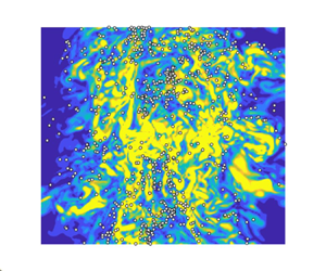
To illustrate the qualitative differences between the particle-laden jets at the three different Stokes numbers, figure 4 presents a slice of the spatial distribution of particles at a single time instance overlapped with the magnitude of the instantaneous gas-phase vorticity. As can be seen, particle clustering in the particle-laden jets with $S{t_D} = 0.3$ and 1.4 is more significant than for $S{t_D} = 11.2$. For $S{t_D} = 0.3$ and 1.4, there is visual evidence of particles tending to concentrate in regions of low vorticity, consistent with expectation (Eaton & Fessler Reference Eaton and Fessler1994). However, there are also exceptions. For these two images, particles within the first few diameters of the inlet are observed to exhibit notable radial dispersion in response to the shear layer roll-ups (Mi, Nobes & Nathan Reference Mi, Nobes and Nathan2001), indicating a strong response to the gas-phase flow field. Meanwhile, for $S{t_D} = 11.2$, the particle locations show much less visual correspondence to the vorticity distribution. Also, for this high Stokes number case, particle clustering is less apparent than at $S{t_D} = 0.3$ and 1.4, and there is almost no radial dispersion within the first few jet diameters, where particles exhibit ballistic behaviour due to their large relaxation time scale compared with the local flow time scale. The observable radial dispersion only starts to occur after $15{D_j}$, consistent with the decrease in the local Stokes number with axial distance (Lau & Nathan Reference Lau and Nathan2016). More work is required to confirm or refine these visual observations with statistical analysis. Appendix D presents the investigation based on a Voronoi diagram, which provides a more quantitative analysis of particle clustering and preferential concentration in the low-vorticity region.

Figure 4. Instantaneous spatial distributions of particles overlaid with the vorticity magnitude normalised by a frequency defined by the inflow jet bulk velocity and jet diameter.

Figure 5 presents the predicted spatial distribution of the ensemble averaged mean particle number density in comparison with the experiment (Lau & Nathan Reference Lau and Nathan2016). For each image pair, the experimentally measured distribution is shown on the left, while the DNS is on the right. The particle number density was measured by using planar nephelometry, which infers the relative particle number density from the intensity of the measured Mie scattering signal (Birzer, Kalt & Nathan Reference Birzer, Kalt and Nathan2012). The particle number density in the DNS was computed as being $\langle \varTheta (\boldsymbol{x})\rangle = \sum\nolimits_{i = 1}^{{N_t}} {[\sum\nolimits_{k = 1}^{N_p^{(i)}} {G(\boldsymbol{x} - \boldsymbol{x}_p^{(k,i)})} ]} /{N_t}$, where ${N_t}$ is the number of time instances used for the statistics, $N_p^{(i)}$ is the number of particles at the ith time instance, $\boldsymbol{x}_p^{(k,i)}$ represents the location of the kth particle at the ith time instance and $G(\boldsymbol{x} - \boldsymbol{x^{\prime}})$ represents a top hat function, which is essentially a cube centred at the location $\boldsymbol{x}$ with its volume corresponding to the local grid cell. As shown, the spatial distribution of the particle number density is well reproduced by the simulations. Specifically, both experiments and the simulations show that, for the two lower Stokes number cases, i.e. $S{t_D} = 0.3$ and 1.4, the region of peak particle number density shifts from the jet edge towards the centreline as the flow convects downstream. Furthermore, the simulations match the experiments in showing that the axial decay rate of particle number density decreases as $S{t_D}$ increases. As the only force term included in the equations of motion is the drag force, the close match between the experiment and simulation implies that incorporating only the drag force is sufficient to reasonably predict the large-scale features of the particle-phase motion for all particle-laden jets considered in this work.

Figure 5. Comparison of the measured (left) and simulated (right) spatial distributions of the mean particle number density ($\langle \varTheta \rangle $) for three values of Stokes number. Experimental data from Lau & Nathan (Reference Lau and Nathan2016).

Figure 6 presents the radial profiles of the mean particle number density at three axial locations, $x/{D_j} = 5.0$, 10.0 and 25.0. As can be seen, the radial profiles of $\langle \varTheta \rangle /\langle {\varTheta _c}\rangle $ for all three Stokes number cases were reproduced quantitatively by the simulations for most cases, although there are some differences. The relative error is less than 12 % in general. Moreover, Gaussian fits are applied to the measured profiles in the experiment, as it is well established that the passive scalar profile of a single-phase jet approaches a Gaussian in the far field (Pope Reference Pope2000). For $S{t_D} = 0.3$, the radial profiles of $\langle \varTheta \rangle /\langle {\varTheta _c}\rangle $ at all three axial locations match the Gaussian profiles reasonably well, especially for $x/{D_j} > 5.0$. Consistent with the findings in the experiment, the simulation results show that, for the case of $S{t_D} = 0.3$, the particles quickly reorganize from being preferentially concentrated at the jet edge (see figure 2b) to being preferentially concentrated towards the jet centreline within the first ~5 diameters of the inlet. For $S{t_D} = 11.2$, the radial profiles exhibit notable deviation from a Gaussian even at downstream distances of $x/{D_j} = 25.0$. These profiles show a steep decline with radial distance near the jet centreline followed by a long tail. In fact, these profiles resemble more the right half of a log-normal profile rather than a Gaussian profile. These findings indicate that the particle number density profile approaches a Gaussian at increasing axial distances as the inlet Stokes number increases, which is consistent with Lau & Nathan (Reference Lau and Nathan2016).

Figure 6. Measured and simulated radial profiles of the mean particle number density ($\langle \varTheta \rangle $) at three different axial locations. Experimental data from Lau & Nathan (Reference Lau and Nathan2016).

Figure 7 presents the radial profiles of the particle-phase mean axial velocity ($\langle {U_{p,x}}\rangle $) at $x/{D_j} = 5.0$, 10.0 and 30.0. As shown, the mean particle-phase velocity is reasonably reproduced by the PP-DNS, especially for the low Stokes number cases, i.e. $S{t_D} = 0.3$ and 1.4. However, for the high Stokes number case of $S{t_D} = 11.2$, the PP-DNS predicts slightly wider radial profiles of $\langle {U_{p,x}}\rangle $ near to the shear layer at $x/{D_j} = 5.0$ and 10.0. The slight overprediction of the particle-phase velocity spread may be attributed to the limitation of the point-particle method, as illustrated in Appendix A. The Stokes number based on the Kolmogorov scale is over 30 before $x/{D_j} = 10.0$, therefore, the point-particle assumption may not be strictly valid at $x/{D_j} = 5.0$ and 10.0 for the case of $S{t_D} = 11.2$. At $x/{D_j} = 30.0$, the numerical and experimental data exhibit better agreement for the case of $S{t_D} = 11.2$. This is consistent both with the quadratic decrease in Stokes number and with the decrease in volumetric loading with the axial distance, both of which will increase the validity of the point-particle approximation.

Figure 7. Radial profiles of the particle-phase mean axial velocity ($\langle {U_{p,x}}\rangle $) at three different axial locations. Experimental data from Lau & Nathan (Reference Lau and Nathan2016).

Figure 8 presents the radial profiles of the particle-phase r.m.s. axial velocity at $x/{D_j} = 5.0, 10.0$ and 30.0, respectively. As expected, the prediction of the r.m.s. velocity is in general less accurate than that of the mean velocity. For $S{t_D} = 0.3$, the relative error is in general less than 10 % at the two selected locations. The relative error increases with the inlet Stokes number, for $S{t_D} = 1.4$ and 11.2, the maximum relative errors at the selected locations are approximately 20 % and 35 %, respectively. For all three cases, the relative error in r.m.s. velocity at $x/{D_j} = 10.0$ is, in general, larger than that at $x/{D_j} = 30.0$. This again points to the limitation of the point-particle assumption.

Figure 8. Radial profiles of the particle-phase r.m.s. axial velocity at three different axial locations. Experimental data from Lau & Nathan (Reference Lau and Nathan2016).

Notwithstanding the potential role of the point-particle approximation, the synthesised inflow turbulence based on the Passot–Pouquet energy spectrum and Taylor's frozen turbulence hypothesis may also be a source of difference between the numerical simulation and the experimental measurement. Nevertheless, the error in the r.m.s. ${U_{p,x}}$ is expected to have a minor impact on the rest of the analyses. Specifically, for the results presented in § 3.2, the first-order impact of particles on the gas-phase TKE is via the mean drag force determined by the gas- and particle-phase mean velocity, which is illustrated to be reasonably well reproduced, as shown in figure 7. In addition, the influence of the r.m.s. ${U_{p,x}}$ on the conditional mean velocity statistics, as well as the integral length scale, is also minor, therefore, the error in r.m.s. ${U_{p,x}}$ has a minor impact on the particle response presented in § 3.3. In general, the PP-DNS results provides a reasonable baseline for the subsequent analysis of turbulence–particle interactions in terms of turbulence modulation and particle response.

3.2. Modulation of turbulence

To investigate turbulence modulation, figure 9 presents the axial evolution of the mean slip velocity to illustrate the region where the particle phase lags or leads the gas phase. The mean slip velocity is computed as $\langle {U_{slip,x}}\rangle = \langle {U_{g,x}}|\boldsymbol{x} = {\boldsymbol{x}_p}\rangle - \langle {U_{p,x}}\rangle $, where $\langle {U_{g,x}}|\boldsymbol{x} = {\boldsymbol{x}_p}\rangle $ represents the conditionally averaged gas-phase velocity at the particle location. Figure 9(a) presents the centreline slip velocity, which is positive in the near-field region. This is because the centreline mean velocity of the gas phase is slightly higher than that of the particle phase at the pipe exit, as a result of the dynamics of the particle-laden pipe flow (Lau & Nathan Reference Lau and Nathan2014, Reference Lau and Nathan2016). The positive slip velocity illustrates that the particle phase lags the gas phase in the near-field region. Downstream of the inlet plane, due to particle inertia, the particle-phase velocity decays at a lower rate than the gas phase. Therefore, the particle-phase velocity eventually exceeds the gas-phase velocity, resulting in a negative slip velocity further downstream. The slip velocity eventually approaches zero in the far field as the local Stokes number decreases, resulting in the particles more faithfully following the flow. Figure 9(b) presents the slip velocity at the location of the gas-phase velocity half-width, which is negative throughout the domain illustrating that, for all three particle-laden jets, the particle phase leads the gas phase at the velocity half-width location within the first $30{D_j}$ from the inlet. Both figure 9(a,b) illustrate that, in the region where the particle phase leads, the higher Stokes number case exhibits a greater (in magnitude) slip velocity due to the higher particle inertia. This results in a larger positive momentum transfer to the gas phase via $\langle {F_{p,x}}\rangle $ (see (2.2)), and therefore, a slower decay of the mean gas-phase velocity for the higher Stokes number cases.

Figure 9. Axial evolution of the slip velocity ($\langle {U_{slip,x}}\rangle $) at the centreline (a) and the velocity half-width location (b). The inset is a zoom in plot for $0 < x/{D_j} < 2$.

To quantify the modulation on turbulence due to the presence of the particle phase, figure 10(a) presents the axial evolution of the normalised gas-phase TKE ($k = \langle {u^{\prime}_{g,i}}{u^{\prime}_{g,i}}\rangle /2$) at the velocity half-width location (${R_{0.5{U_{g,x - c}}}}$) for the single-phase jet together with the particle-laden jet at all three Stokes numbers. Compared with the single-phase jet, the gas-phase TKE in the particle-laden jet is damped for $x < 5{D_j}$ for all three Stokes numbers. The low Stokes number cases, i.e. $S{t_D} = 0.3$ and 1.4, yield much more significant damping relative to $S{t_D} = 11.2$. Specifically, $S{t_D} = 0.3$ and 1.4 reduce the peak value of TKE by approximately 30 % compared with the single phase, while $S{t_D} = 11.2$ results in only minor damping of less than 5 %. In the intermediate region, $5{D_j} < x < 20{D_j}$, the gas-phase TKE in the particle-laden jet is greater than that of the single-phase jet for all Stokes numbers. The level of increase appears to be less dependent on the Stokes number, i.e. 15 %–25 % for all the three cases considered. The increase of the gas-phase TKE persists to the end of the computational domain as the presence of the particle phase slows down the decay of the gas-phase TKE owing to the higher particle inertia (see figure 14 for further discussion).

Figure 10. Axial variation of the normalised gas-phase TKE, variance of axial and radial velocities ($\langle u^{\prime 2}_{g,x}\rangle $ and $\langle u^{\prime 2}_{g,r}\rangle $) at the velocity half-width location (${R_{0.5{U_{g,x - c}}}}$), for the single-phase case and the particle-laden cases $S{t_D} = 0.3$, 1.4 and 11.2. The y-axis is normalised by the square of the inflow jet bulk velocity.

Figure 10(b,c) presents the normalised variance of the gas-phase velocity component in the axial and radial directions. For $x < 5{D_j}$, the presence of the particle phase damps the fluctuating velocity in both the axial and radial directions, especially for low Stokes number cases. For example, the peak values of $\langle u^{\prime 2}_{g,r}\rangle $ and $\langle u^{\prime 2}_{g,x}\rangle$ for the $S{t_D} = 0.3$ and 1.4 cases are approximately 40 % and 20 % lower than the corresponding peak values for the single-phase case. The significant radial damping in this region ($x < 5{D_j}$) may be attributed to the reorganisation of the particle concentration towards a Gaussian-like profile (Lau & Nathan Reference Lau and Nathan2016), with this reorganisation being expected to occur at a greater rate for the two lower Stokes number cases due to the highly non-Gaussian initial particle distributions for these cases (see figure 5). In the intermediate region of $5{D_j} < x < 20{D_j}$, the presence of the particle phase increases both $\langle u^{\prime 2}_{g,x}\rangle $ and $\langle u^{\prime 2}_{g,r}\rangle $. However, $\langle u^{\prime 2}_{g,x}\rangle $ is increased more significantly. For all three particle-laden jets, the increase of $\langle u^{\prime 2}_{g,x}\rangle $ is around 35 %, which is notably larger than the 20 % increase for $\langle u^{\prime 2}_{g,r}\rangle $. The preferential increase of the gas-phase fluctuating velocity in the axial direction is consistent with the preferential axial response of the particle phase owing to the lower characteristic Stokes number in axial direction (see § 3.4 for detailed discussion). The increase of $\langle u^{\prime 2}_{g,x}\rangle $ and $\langle u^{\prime 2}_{g,r}\rangle $ persists to the end of the computational domain. As far as turbulence anisotropy is concerned, the single-phase jet exhibits significant anisotropy, as indicated by $\langle u^{\prime 2}_{g,x}\rangle /\langle u^{\prime 2}_{g,r}\rangle$ being larger than unity. Specifically, the ratio of $\langle u^{\prime 2}_{g,x}\rangle /\langle u^{\prime 2}_{g,r}\rangle $ at the velocity half-width location is ~1.4, which is consistent with previous single-phase experimental measurements (Hussein, Capp & George Reference Hussein, Capp and George1994). The presence of the particle phase causes the preferential damping of $\langle u^{\prime 2}_{g,r}\rangle $ in the near field and the preferential increase of $\langle u^{\prime 2}_{g,x}\rangle $ in the intermediate region which, therefore, results in an overall higher anisotropy than for the single-phase jet. For example, the anisotropy indicated by the ratio of $\langle u^{\prime 2}_{g,x}\rangle /\langle u^{\prime 2}_{g,r}\rangle $ at the velocity half-width location of $x = 20{D_j}$ is 1.6, 1.9 and 2.0 for $S{t_D} = 0.3$, 1.4 and 11.2, respectively.

Given the strong spatial variation in the gas-phase TKE, figure 11 presents the normalised TKE radial at three representative locations corresponding to the near, intermediate and ‘far’ fields, i.e. $x/{D_j} = 1.5$, 15.0 and 25.0, respectively. Note that previous work (Mi et al. Reference Mi, Nobes and Nathan2001) has shown that true similarity of the far field for both the mean and r.m.s. quantities for a single-phase jet is not reached until $x/{D_j} = 70$, although the equivalent data are not available for a two-phase jet. As shown, compared with the single-phase jet, the gas-phase TKE is in general damped in the near field of the particle-laden jets, especially for $S{t_D} = 0.3$ and 1.4, and then increased in the intermediate field, consistent with the results presented in figure 10. The increase of the gas-phase TKE persists to the end of the computational domain, for example, at $x/{D_j} = 25$, the increase in the magnitude of the peak TKE for $S{t_D} = 0.3$ is around 10 % of its single-phase counter part, while that for $S{t_D} = 1.4$ and 11.2 is more than 20 %.

Figure 11. Radial profiles of the normalised gas-phase TKE at $x/{D_j} = 1.5$, 15.0 and 25.0, for the single-phase case and the particle-laden cases for $S{t_D} = 0.3$, 1.4 and 11.2. The TKE is normalised by the square of the inflow jet bulk velocity.

In addition to TKE, the radial profiles of Reynolds stress components, $\langle {u^{\prime}_{g,x}}{u^{\prime}_{g,x}}\rangle $, $\langle {u^{\prime}_{g,r}}{u^{\prime}_{g,r}}\rangle $ and $\langle {u^{\prime}_{g,x}}{u^{\prime}_{g,r}}\rangle $, are presented to provide more details about the modulation of turbulence. Figure 12 presents the radial profiles of the gas-phase Reynolds stress components, $\langle {u^{\prime}_{g,x}}{u^{\prime}_{g,x}}\rangle $, $\langle {u^{\prime}_{g,r}}{u^{\prime}_{g,r}}\rangle$ and $\langle {u^{\prime}_{g,x}}{u^{\prime}_{g,r}}\rangle$ at $x/{D_j} = 1.5$ and 25. As can be observed, the variation of the Reynolds stress due to the presence of the particle phase strongly depends on the inlet Stokes number.

Figure 12. Radial profiles of the normalised Reynolds stresses, i.e. $\langle {u^{\prime}_{g,x}}{u^{\prime}_{g,x}}\rangle $, $\langle {u^{\prime}_{g,r}}{u^{\prime}_{g,r}}\rangle $ and $\langle {u^{\prime}_{g,x}}{u^{\prime}_{g,r}}\rangle $ at $x/{D_j} = 1.5$ (a) and 25 (b), for the single-phase jet and the particle-laden jets $S{t_D} = 0.3$, 1.4 and 11.2. The y-axis is normalised by the square of the inflow jet bulk velocity.

The results at $x/{D_j} = 1.5$ show that the profiles of the Reynolds stresses for all Stokes number cases, as well as the single-phase case, have a peak in the shear layer ($r/{D_j} = 0.5$), consistent with expectation. Furthermore, the three components of Reynolds stress in the particle-laden jets are lower than the single-phase jet. This illustrates that the presence of particles damps the Reynolds stresses, with the damping of $\langle {u^{\prime}_{g,r}}{u^{\prime}_{g,r}}\rangle $ is more significant than that of $\langle {u^{\prime}_{g,x}}{u^{\prime}_{g,x}}\rangle $ and $\langle {u^{\prime}_{g,x}}{u^{\prime}_{g,r}}\rangle $. Taking $S{t_D} = 1.4$ as an example, the peak values of $\langle {u^{\prime}_{g,x}}{u^{\prime}_{g,x}}\rangle $ and $\langle {u^{\prime}_{g,x}}{u^{\prime}_{g,r}}\rangle $ are 21 % and 26 % lower than the single-phase jet, respectively, while the peak value of $\langle {u^{\prime}_{g,r}}{u^{\prime}_{g,r}}\rangle $ is as much as 37 % lower than the single-phase jet. These findings are consistent with previously published experimental results, which showed that particles tend to preferentially respond to the axial fluctuations in the gas-phase velocity compared with the radial fluctuations (Lau & Nathan Reference Lau and Nathan2014). As the inlet Stokes number is increased, the three Reynolds stress components approach the corresponding ones in the single-phase jet, illustrating that larger particles have less impact on the gas-phase velocity in the near-field region. This is attributed to the decrease of the overall particle drag as the inlet Stokes number is increased (as later analysed in figure 13).

Figure 13. Radial profiles of the normalised TKE budgets at $x/{D_j} = 1.5$, for the single-phase case and the particle-laden cases $S{t_D} = 0.3$, 1.4 and 11.2. The y-axis is normalised by a rate defined by the inflow jet bulk velocity and jet diameter ($U_{g,x - b - e}^3/{D_j}$).

Figure 14. Radial profiles of the normalised TKE budgets at $25.0{D_j}$, for the single-phase case and the particle-laden cases $S{t_D} = 0.3$, 1.4 and 11.2. The y-axis is normalised by a rate defined by the inflow jet bulk velocity and jet diameter ($U_{g,x - b - e}^3/{D_j}$).

At $x/{D_j} = 25$, the three Reynolds stress components in the particle-laden jet are higher than those in the single-phase jet for all Stokes numbers. This is because the Reynolds stress decays more slowly in the particle-laden jet than the single-phase jet due to the greater inertia in the former. The peak magnitude of the Reynolds stress consistently increases with the inlet Stokes number, which is consistent with the later findings from figure 14. In addition, the increase of $\langle {u^{\prime}_{g,x}}{u^{\prime}_{g,x}}\rangle $ and $\langle {u^{\prime}_{g,x}}{u^{\prime}_{g,r}}\rangle $ is more significant than that of $\langle {u^{\prime}_{g,r}}{u^{\prime}_{g,r}}\rangle $. Taking $S{t_D} = 1.4$ as an example, the peak value of $\langle {u^{\prime}_{g,r}}{u^{\prime}_{g,r}}\rangle $ is 40 % higher than the single-phase jet, while the peak values of $\langle {u^{\prime}_{g,x}}{u^{\prime}_{g,x}}\rangle $ and $\langle {u^{\prime}_{g,x}}{u^{\prime}_{g,r}}\rangle $ are as much as 55 % and 50 % higher than the single-phase jet, respectively.

To better explain the modulation of turbulence by the presence of the particle phase, a budget analysis of TKE is carried out. The transport equation of the gas-phase TKE ($k$) in particle-laden flows yields (Pope Reference Pope2000; Li et al. Reference Li, Luo, Wang, Xiao and Fan2019):

(3.1)\begin{equation}\frac{{\partial k}}{{\partial t}} ={-} \langle {U_{g,i}}\rangle \frac{{\partial k}}{{\partial {x_i}}} + {P_k} + {\epsilon _k} + {S_k} + {D_k},\end{equation}

where ${P_k}$ represents the production term, ${\epsilon _k}$ represents the dissipation term and ${S_k}$ is a source term due to the presence of the particle phase. The other terms, i.e. turbulent convection, viscous diffusion and pressure transport are lumped to ${D_k}$,

(3.2)\begin{gather}{P_k} ={-} \langle {u^{\prime}_{g,i}}{u^{\prime}_{g,j}}\rangle \frac{{\partial \langle {U_{g,i}}\rangle }}{{\partial {x_j}}},\end{gather}

(3.3)\begin{gather}{\epsilon _k} ={-} 2{\nu _g}\langle {s^{\prime}_{g,ij}}{s^{\prime}_{g,ij}}\rangle ={-} {\nu _g}\left\langle {\frac{{\partial {{u^{\prime}}_{g,i}}}}{{\partial {x_j}}}\left( {\frac{{\partial {{u^{\prime}}_{g,i}}}}{{\partial {x_j}}} + \frac{{\partial {{u^{\prime}}_{g,j}}}}{{\partial {x_i}}}} \right)} \right\rangle ,\end{gather}

(3.4)\begin{gather}{S_k} = \langle {f^{\prime}_i}\,{u^{\prime}_{g,i}}\rangle ,\end{gather}

(3.5)\begin{gather}{D_k} ={-} \frac{1}{2}\frac{{\langle \partial {{u^{\prime}}_{g,j}}{{u^{\prime}}_{g,i}}{{u^{\prime}}_{g,i}}\rangle }}{{\partial {x_j}}} - \frac{1}{{{\rho _g}}}\frac{{\partial \langle {{p^{\prime}}_g}{{u^{\prime}}_{g,j}}\rangle }}{{\partial {x_j}}} + {\nu _g}\frac{{{\partial ^2}k}}{{\partial {x_j}\partial {x_j}}},\end{gather}

where ${u^{\prime}_{g,i}}$ and ${f^{\prime}_i}$ represents fluctuating components of the velocity and the particle-induced force, while ${U_{g,i}}$ represents the total instantaneous gas-phase velocity component. Einstein notation is applied to the repeated indices. Note that the influence of the particle volume on the gas-phase TKE is neglected as the particle-phase volume fraction is negligibly low, i.e. ${\sim} {10^{ - 4}}$. The dissipation term (${\epsilon _k}$) is computed as the dissipation rate based on the total instantaneous velocity (${\boldsymbol{U}_g}$) minus the dissipation rate based on the mean velocity ($\langle {\boldsymbol{U}_g}\rangle $). The lumped diffusion term (${D_k}$) is mostly responsible for spatially transferring TKE within the gas-phase itself, while not making a direct contribution to turbulence increase or reduction (Li et al. Reference Li, Luo, Wang, Xiao and Fan2019). In the following, the budget analysis mostly focuses on the source and sink terms, i.e. ${P_k}$, ${\epsilon _k}$ and ${S_k}$. As illustrated in (3.1), the gas-phase TKE is influenced by the particle phase directly via the source term ${S_k}$, and indirectly via ${P_k}$ and ${\epsilon _k}$ through the particles’ influence on the gas-phase velocity field.

Figure 13 presents the radial profiles of the normalised TKE budget in the jet near field, $x/{D_j} = 1.5$. As can be seen, the production and dissipation terms reach their peak magnitudes near to the shear layer region (${\sim} r/{D_j} = 0.5$) for both the single-phase jet and the particle-laden jets. Compared with the single-phase jet, the presence of particles results in a notably reduced production term (${P_k}$), especially for cases with small particles, i.e. $S{t_D} = 0.3$ and 1.4. This is because the presence of particles reduces the spatial gradient of the gas-phase mean velocity. More specifically, the gas velocity within the upstream pipe is lower than the particle phase in the near-wall region ($r/{D_j} > 0.4$), due to viscous drag from the pipe wall, but higher than the particle phase in the core of the jet. Once the particle-laden flow leaves the pipe, the particle phase retains a similar velocity due to its higher inertia. Therefore, in the near-field region, the particle phase lags the gas phase in the high-speed jet core, but leads it near to the low-speed jet edge, resulting in a decrease of the main component of the velocity gradient, i.e. $\partial \langle {U_{g,x}}\rangle /\partial r$, relative to the single phase, and thus to a decrease in ${P_k}$.

It can also be seen that the peak magnitudes of ${P_k}$ and ${\epsilon _k}$ are notably reduced for the low Stokes number cases of $S{t_D} = 0.3$ and 1.4, but almost unchanged for the highest Stokes number case ($S{t_D} = 11.2$). The stronger reduction of ${P_k}$ and ${\epsilon _k}$ by the smaller particles can be qualitatively explained by calculating the magnitude of the particle drag force (${\boldsymbol{F}_p}$). By definition, $|{{\boldsymbol{F}_p}} |\; \sim \; m_p^0 \times {\varTheta _b}/{\tau _p} \times |{{\boldsymbol{U}_{slip}}} |\times {\varTheta ^\mathrm{\ast }}$, where $|{{\boldsymbol{U}_{slip}}} |$ is the magnitude of the local slip velocity and ${\varTheta ^\mathrm{\ast }}$ is the local particle number density normalised by the bulk number density (${\varTheta _b}$). The product of the first three terms scales as $1/d_p^2$, so that $|{{\boldsymbol{F}_p}} |\sim|{{\boldsymbol{U}_{slip}}} |\times {\varTheta ^\mathrm{\ast }}/d_p^2$. At the location of $x/{D_j} = 1.5$ and $r/{D_j} = 0.5$, even though $S{t_D} = 11.2$ has a value of $|{{\boldsymbol{U}_{slip}}} |$ that is some 15 times greater than for $S{t_D} = 0.3$, this is more than offset by the fortyfold increase in $d_p^2$. Moreover, $S{t_D} = 0.3$ has a value of ${\varTheta ^\mathrm{\ast }}$ which is 2.5 times greater than for $S{t_D} = 11.2$. Combining all these, $|{{\boldsymbol{F}_p}} |$ for $S{t_D} = 0.3$ is around 6 times higher than for $S{t_D} = 11.2$ in the near field, which explains why smaller particles have a stronger impact on the gas-phase velocity in the near-field region and thus also a stronger reduction of ${P_k}$ and ${\epsilon _k}$.

The particle-induced source term (${S_k}$) is negative for all three particle-laden cases, indicating that the direct impact of the particle phase is to dissipate the gas-phase TKE. The previous analysis also applies here to explain that the magnitude of ${S_k}$ for $S{t_D} = 11.2$ is much smaller than that for $S{t_D} = 0.3$ and 1.4. It is worth noting that, for the low Stokes number cases $S{t_D}$=0.3 and 1.4, the magnitude of ${S_k}$ is comparable to that of the dissipation term (${\epsilon _k}$), illustrating that the particles under these conditions play an important role in dissipating TKE. That is, in addition to the reduction of ${\epsilon _k}$ due to the presence of the particle phase, further dissipation of similar order is provided through ${S_k}$. Nevertheless, the total dissipation, i.e. ${\epsilon _k} + {S_k}$ is approximately the same as that of ${\epsilon _k}$ for the single-phase jet. Meanwhile, the production term is reduced in particle-laden jets due to the decrease of the mean velocity gradient. Therefore, the reduction of the near-field TKE in particle-laden jets is mostly due to the reduction of the overall production, rather than the increase of the total dissipation. Furthermore, the level of reduction for ${P_k}$ increases monotonically as the inlet Stokes number is reduced. This explains why $S{t_D} = 0.3$ yields the most significant damping, while $S{t_D} = 11.2$ yields the least damping for gas-phase TKE in the near field. Note that figure 13 only presents the source terms, i.e. ${P_k}$, ${\epsilon _k}$ and ${S_k}$ for clarity, and this results in obviously imbalanced TKE budgets. Figure 25 in Appendix B presents the balanced TKE budgets by including the lumped diffusion term ($D_k$) and the transport term due to mean convection.

Figure 14 presents the radial profiles of the normalised TKE budget at the downstream location of $x/{D_j} = 25$. For the single-phase jet, the production term reaches its peak magnitude near to the shear layer, while the dissipation term exhibits a flat profile from the centreline to the shear layer region, consistent with previous measurements in a turbulent single-phase jet (Hussein et al. Reference Hussein, Capp and George1994). Compared with the single-phase case, the peak magnitudes of ${P_k}$ and ${\epsilon _k}$ are increased in particle-laden jets. This is because the particle phase leads the gas phase downstream of $25\; {D_j}$ (see figure 9), increasing the momentum of the gas phase. The positive momentum transfer slows down the decay of the gas-phase velocity and its gradients. This, then, results in greater values of ${P_k}$ and ${\epsilon _k}$ at a given downstream location than for the single-phase case. Since the higher Stokes number case yields a slower decay of both the gas-phase velocity and its gradients, owing to the higher particle inertia, this explains the consistent increase in the peak magnitudes of ${P_k}$ and ${\epsilon _k}$ with the inlet Stokes number.

The particle-induced source term (${S_k}$) remains negative at $25{D_j}$ for all three particle-laden cases. It is worth noting that the particle phase leads the gas phase at $25{D_j}$, as illustrated by the negative mean slip velocity shown in figure 9. However, ${S_k}$ remains negative. This seemingly counterintuitive finding is because the mean slip velocity determines the mean quantities, e.g. mean drag and mean kinetic energy, but not the fluctuating quantities such as ${S_k}$, which is defined as the product of fluctuating drag and fluctuating gas-phase velocity (${S_k} = \langle {f^{\prime}_i}{u^{\prime}_{g,i}}\rangle $). By its definition, there is not a one-to-one correspondence between the sign of the mean slip velocity and the sign of ${S_k}$. The negative ${S_k}$ illustrates that the particle phase continues to play a role in dissipating gas-phase TKE. This confirms that there is no positive TKE transfer from the particle to the gas phase. Instead, the increase of the intermediate-field TKE in particle-laden jets also results mostly from the slower decay of the gas-phase velocity. As discussed above, a higher Stokes number case maintains the axial momentum of the gas phase for a longer distance which, in turn, results in the $S{t_D} = 11.2$ case yielding the most prominent increase, while the $S{t_D} = 0.3$ case yields the least increase for the gas-phase TKE in the intermediate field.

3.3. Direction-dependent response of the particle phase

Figure 15 presents scatter plots of the instantaneous axial particle-phase velocity as a function of the gas-phase velocity at the corresponding particle location. Data are reported at the velocity half-width location ($r = {R_{0.5{U_{g,x - c}}}}$) at $x/{D_j} = 15$. Also drawn is a reference line of ${U_{p,x}} = {U_{g,x}}$, representing the perfect response of particles to the flow field. As expected, particles of $S{t_D} = 0.3$ and $S{t_D} = 1.4$ exhibit notably stronger response than those of $S{t_D} = 11.2$. It can be seen that the data are skewed, with the particle phase tending to lead the gas phase, which is expected to occur at the velocity half-width location throughout the computational domain (see figure 9). Furthermore, the skewness increases with $S{t_D}$.

Figure 15. Scatter of the instantaneous particle velocity versus the gas velocity at the corresponding particle location. Samples were taken at the velocity half-width location at $x/{D_j} = 15$, with a sampling region of $0.2{D_j}$ and $0.5{D_j}$ in the r and x directions, respectively.

The probability density function (PDF) of the ${U_{p,x}}/{U_{g,x}}$ is shown in figure 16. Data are reported at the velocity half-width locations at $x/{D_j} = 5.0$, 15.0 and 25.0. Consistent with the findings from figure 15, the PDF in $S{t_D} = 0.3$ is very narrow, with values close to 1.0, while the PDF becomes boarder with an increase in the Stokes number given an axial distance, consistent with the fact that the particle response increases as the Stokes number is reduced. The trend in skewness observed in figure 15 is better illustrated here. Specifically, the distribution of ${U_{p,x}}/{U_{g,x}}$ is skewed to the side greater than unity. This can be explained by figure 9, in which the particle phase is shown to lead the gas phase in the intermediate-field region owing to the higher particle inertia there, resulting in a large number of samples having ${U_{p,x}}/{U_{g,x}}$ greater than unity. Since larger particles have higher inertia, this explains why the distribution of ${U_{p,x}}/{U_{g,x}}$ is more skewed in the particle-laden jet with higher inlet Stokes number. The skewness reduces with downstream distance following the corresponding decrease in local Stokes number.

Figure 16. Probability density function of the ratio ${U_{p,x}}/{U_{g,x}}$. Samples were taken at the velocity half-width location at $x/{D_j} = 15$, with a sampling region of 0.2$D_j$ and 0.5$D_j$ in the r and x directions, respectively.

To quantify the level of particle response, the conditionally averaged particle velocity ($\langle {U_{p,i}}|{U_{g,i}}\rangle $) is plotted as a function of the gas velocity at the particle location for a series of axial distances and at radial locations corresponding to the velocity half-width. To compute $\langle {U_{p,i}}|{U_{g,i}}\rangle $ numerically, ${U_{g,i}}$ is divided into 100 bins, and the ensemble average of ${U_{p,i}}$ is calculated within each bin. A perfect particle response would result in $\langle {U_{p,i}}|{U_{g,i}}\rangle = {U_{g,i}}$. In figure 17(a), $\langle {U_{p,x}}|{U_{g,x}}\rangle $ is plotted against ${U_{g,x}}$ to present the particle response in the axial direction, while in figure 17(b), $\langle {U_{p,r}}|{U_{g,r}}\rangle $ is plotted against ${U_{g,r}}$ to present the particle response in the radial direction. The linear regression for each direction was also calculated, such that the slope, i.e. ${K_{{U_x}}} = \arg {\min _K}\parallel K{U_{g,x}} + {b_x} - \langle {U_{p,x}}|{U_{g,x}}\rangle {\parallel _2}$ or ${K_{{U_r}}} = \arg {\min _K}\parallel K{U_{g,r}} + {b_r} - \langle {U_{p,r}}|{U_{g,r}}\rangle {\parallel _2}$, measures how strongly the particle-phase velocity is correlated to the gas-phase velocity in the corresponding direction, with a value of unity meaning perfect correlation, and a value of zero meaning no correlation. It can be seen that both the axial and radial particle responses increase consistently with the axial distance, as indicated by the observation that ${K_{{U_x}}}$ and ${K_{{U_r}}}$ approach unity. This is expected because the local Stokes number decreases with the square of axial distance.

Figure 17. Conditionally averaged particle velocity as a function of gas velocity at the corresponding particle location for a series of axial distances and at radial locations corresponding to the velocity half-width (where the sampling region is 0.2$D_j$ and 0.5$D_j$ in the r and x directions, respectively). (a) Axial velocity component; (b) radial velocity component. The dashed black lines are linear fits of the data. The dot-dashed lines represent the reference of unity slope.

Figure 18 presents the axial variation of the dimensionless particle response indicated by ${K_{{U_x}}}$ and ${K_{{U_r}}}$. Figure 18(a) presents the values of ${K_{{U_x}}}$ and ${K_{{U_r}}}$ obtained at the velocity half-width location for the three particle-laden jets. As can be observed, for a given axial distance, the values of ${K_{{U_x}}}$ and ${K_{{U_r}}}$ approach unity with a decrease in the values of the inlet Stokes number. Moreover, ${K_{{U_x}}}$ and ${K_{{U_r}}}$ both increase with axial distance, which is as expected given that the local Stokes number decreases with ${x^{ - 2}}$. Furthermore, ${K_{{U_x}}}$ is closer to unity than ${K_{{U_r}}}$ for a given axial distance in all three particle-laden jets, illustrating the direction-dependent response of particles to the axial gas-phase velocity component in comparison with the radial component. For example, for $S{t_D} = 0.3$, ${m_x}$ exceeds 0.95 as near to the inlet plane as $x/{D_j} = 5$, indicating a close response to the axial gas-phase velocity. However, ${K_{{U_r}}}$ is only 0.8 at the same axial distance ($x/{D_j} = 5$), and only exceeds 0.95 for $x > 20{D_j}$. Interestingly, the value of ${K_{{U_r}}}$ is as low as ~0.07 in the near field for the case where $S{t_D} = 11.2$. This implies that the particles have a near-zero correlation to the radial gas velocities near the inlet, particularly for large Stokes numbers.

Figure 18. Axial variation of the particle response, as indicated by ${K_{{U_x}}}$ and ${K_{{U_r}}}$. Samples taken from (a) the velocity half-width; and (b) the centreline.

Figure 18(b) presents the corresponding results sampled along the centreline as for those presented along the half-width in figure 18(a). Comparing these figures shows that some differences in the particle response, as indicated by ${K_{{U_x}}}$ and ${K_{{U_r}}}$, occur for the two radial locations. This is as expected since the particle response depends on the characteristic flow time scale and the local particle concentration, both of which vary radially. However, the key conclusions remain the same, i.e. the particle response improves with an increase in axial distance and a decrease in Stokes number, with the particle phase preferentially responding more to the axial velocity than the radial velocity. The preferential axial response implies a larger characteristic time scale of the gas-phase flow field in the axial direction than in the radial direction (Lau & Nathan Reference Lau and Nathan2016), which results in a smaller characteristic Stokes number in the axial direction.

To compute the characteristic Stokes number in the axial and radial directions ($S{t_{{l_{t,x}}}}$ and $S{t_{{l_{t,r}}}}$), the characteristic flow time scale in these two directions is defined based on the axial and radial integral length scales, respectively, i.e. $S{t_{{l_{t,x}}}}(x) = {\tau _p}/({l_{t,x}}(x,0)/\langle {U_{g,x - c}}(x)\rangle )$ and $S{t_{{l_{t,r}}}}(x) = {\tau _p}/({l_{t,r}}(x,0)/\langle {U_{g,x - c}}(x)\rangle )$, where ${l_{t,x}}(x,0)$ and ${l_{t,r}}(x,0)$ represent the axial and radial integral length scales on the centreline, and $\langle {U_{g,x - c}}(x)\rangle $ is the centreline mean axial velocity. The integral length scale is computed by integrating the velocity auto-correlation function, i.e. ${l_{t,x}}(x,r) = \int_0^\infty {{R_{11}}(\mathrm{\Delta }x;x,r)(\mathrm{d\Delta }x)} $ and ${l_{t,r}}(x,r) = \int_0^\infty {{R_{12}}(\mathrm{\Delta }r;x,r)(\mathrm{d\Delta }r)} $. Following the definition of the velocity auto-correlation function (Pope Reference Pope2000), ${R_{11}}(\mathrm{\Delta }x;x,r)$ and ${R_{12}}(\mathrm{\Delta }r;x,r)$ are computed as

(3.6)\begin{gather}{R_{11}}(\mathrm{\Delta }x;x,r) = \langle {u^{\prime}_{g,x}}(x + \mathrm{\Delta }x,r){u^{\prime}_{g,x}}(x,r)\rangle /\langle {u^{\prime}_{g,x}}(x,r){u^{\prime}_{g,x}}(x,r)\rangle ,\end{gather}

(3.7)\begin{gather}{R_{12}}(\mathrm{\Delta }r;x,r) = \langle {u^{\prime}_{g,x}}(x,r + \mathrm{\Delta }r){u^{\prime}_{g,x}}(x,r)\rangle /\langle {u^{\prime}_{g,x}}(x,r){u^{\prime}_{g,x}}(x,r)\rangle ,\end{gather}

where ${u^{\prime}_{g,x}}(x,r)$ is the gas-phase fluctuating axial velocity at the location $(x,r)$. Figure 19 presents the velocity auto-correlation functions on the centreline at $x/{D_j} = 20.0$, i.e. ${R_{11}}(\mathrm{\Delta }x;20{D_j},0)$ and ${R_{12}}(\mathrm{\Delta }r;20{D_j},0)$. It is known that statistical error can pollute auto-correlation functions at large separation distances, which prevents the accurate calculation of the integral length scale where integration to infinity is used. Therefore, exponential fits were employed for the raw data following previous work (Bewley, Chang & Bodenschatz Reference Bewley, Chang and Bodenschatz2012). As can be seen, $S{t_D} = 0.3$ yields a slightly broader distribution of ${R_{11}}$, while $S{t_D} = 1.4$ and 11.2 yield notably narrower ${R_{11}}$ than for the single-phase jet. Specifically, ${R_{11}}$ drops to below 0.1 for $\mathrm{\Delta }x/{D_j} > 1.7$, 1.9, 0.74, and 0.92 in the single-phase jet and the particle-laden jet with $S{t_D} = 0.3$, 1.4 and 11.2, respectively. The same trend is observed for ${R_{12}}$. Furthermore, ${R_{12}}$ is notably narrower than ${R_{11}}$, with the former dropping to below 0.1 for $\mathrm{\Delta }r/{D_j} > 0.54$, 0.72, 0.32, and 0.34 in single-phase jet and particle-laden jets with $S{t_D} = 0.3$, 1.4 and 11.2, respectively. The narrower ${R_{12}}$ compared with ${R_{11}}$, implies that the integral length scale in radial direction (${l_{t,r}}$) is smaller than its axial counterpart (${l_{t,x}}$). This is illustrated further in figure 20.

Figure 19. Log-normal fitted velocity auto-correlation functions on centreline at $x/{D_j} = 20.0$, where markers represent the raw data and lines represent the exponential fit: (a) ${R_{11}}(\mathrm{\Delta }x;20{D_j},0)$; (b) ${R_{12}}(\mathrm{\Delta }r;20{D_j},0)$.

Figure 20. Axial variations of three measures of the centreline integral length scale: (a) axial integral length scale (${l_{t,x}}$); (b) radial integral length scale (${l_{t,r}}$); (c) ratio of ${l_{t,r}}/{l_{t,x}}$.

Figure 20(a,b) presents the axial evolution of the centreline integral length scales in the axial and radial directions, respectively, i.e. ${l_{t,x}}(x,0)$ and ${l_{t,r}}(x,0)$. Since ${l_{t,x}}$ and ${l_{t,r}}$ are determined from the integration of a two-point correlation function, its statistical convergence requires many more sample points than do single-point quantities. Although the results presented in figure 20 have not reached full statistical convergence, the convergence in figure 20(a,b) is sufficient to show that ${l_{t,x}}$ is larger than the corresponding ${l_{t,r}}$ throughout the entire domain. Furthermore, the particle-laden case with $S{t_D} = 0.3$ generally follows that of the single-phase jet, while the cases of $S{t_D} = 1.4$ and 11.2 exhibit notably different profiles at $15.0 < x/{D_j} < 25.0$ compared with their single-phase counterpart. Moreover, figure 20(c) shows that the ratio of ${l_{t,r}}/{l_{t,x}}$ is mostly below 0.5 at all selected locations. The larger integral length scale in the axial direction results in a smaller characteristic Stokes number in the axial direction compared with that in the radial direction. As an indicator of isotropy, ${l_{t,r}}/{l_{t,x}} = 0.5$ corresponds to isotropic turbulence (Pope Reference Pope2000). Due to the anisotropic nature of the shear-driven turbulence in a turbulent jet, ${l_{t,r}}/{l_{t,x}}$ is mostly below 0.5.

Figure 21 presents the axial variation of the local Stokes numbers based on the integral scale in the axial and radial directions, i.e. $S{t_{{l_{t,x}}}}$ and $S{t_{{l_{t,r}}}}$, respectively. The dashed lines are quadratic functions to show that $S{t_{{l_{t,x}}}}$ and $S{t_{{l_{t,r}}}}$ reduce quadratically with axial distance. As a result of the larger integral length scale in the axial direction, $S{t_{{l_{t,x}}}}$ is in general less than half that of the corresponding $S{t_{{l_{t,r}}}}$. This explains the preferential particle response in the axial direction.

Figure 21. Axial variation of the characteristic local Stokes number based on the integral scale in the axial and radial directions, $S{t_{{l_{t,x}}}}$ and $S{t_{{l_{t,r}}}}$: (a) $S{t_D} = 0.3$ and 1.4; (b) $S{t_D} = 11.2$.

Figure 22 combines the results of all three Stokes number cases and presents the particle response indicated by ${K_{{U_x}}}$ and ${K_{{U_r}}}$ as a function of the axial and radial Stokes numbers ($S{t_{{l_{t,x}}}}$ and $S{t_{{l_{t,r}}}}$), respectively. Specifically, figure 22(a,b) presents the ${K_{{U_x}}}$ and ${K_{{U_r}}}$ computed from particles at the centreline and velocity half-width locations, respectively. As can be seen, the two profiles of ${K_{{U_x}}}$ versus $S{t_{{l_{t,x}}}}$ and of ${K_{{U_r}}}$ versus $S{t_{{l_{t,r}}}}$ collapse reasonably well, especially for local Stokes numbers less than 20. This illustrates that the current definitions of $S{t_{{l_{t,x}}}}$ and $S{t_{{l_{t,r}}}}$ qualitatively describe the particle response in the sense that the particle phase would exhibit a similar level of response in the axial and radial directions given the same $S{t_{{l_{t,x}}}}$ and $S{t_{{l_{t,r}}}}$, i.e. the particle response itself is independent of the direction, and the differences in particle behaviour are attributable to differences in the fluid time scale in the axial and radial directions. Nevertheless, despite the use of these directional Stokes numbers, ${K_{{U_x}}}$ still has greater values than ${K_{{U_r}}}$, particularly at high Stokes numbers, implying that the directional Stokes numbers used here do not fully capture the anisotropy in the flow. This implies that the particle response as indicated by ${K_{{U_x}}}$ and ${K_{{U_r}}}$ depends on additional parameters to the local flow time and length scales, such as the local mass loading and the history of particle–fluid interaction. Additionally, it should also be noted that, in a turbulent jet, a range of turbulence scales are present at any given location within the flow. Therefore, while the local Stokes number is one measure of the particle response, it is necessary to incorporate additional parameters to fully characterise the particle response.

Figure 22. Particle response indicated by ${K_{{U_x}}}$ and ${K_{{U_r}}}$ as a function of $S{t_{{l_{t,x}}}}$ and $S{t_{{l_{t,r}}}}$, respectively. Samples taken from (a) the centreline; and (b) the velocity half-width location.