


1. Introduction
Rayleigh–Bénard convection (RBC) refers to natural convection in a horizontal fluid layer caused by unstable vertical temperature stratification and is a fundamental flow system that creates large-scale fluid motion in both nature and industry. Convection is dominated by two dimensionless numbers, the Rayleigh number,  $Ra = g\beta \Delta TL^3/(\kappa \nu )$, and the Prandtl number,
  $Pr = \nu /\kappa$, and the shape and size of the fluid layer, where
  $g$,
$g$,  $\Delta T$ and
  $L$ denote the acceleration due to gravity, vertical temperature difference and height of the fluid layers, respectively, and
  $\beta$,
  $\kappa$ and
  $\nu$ are the thermal expansion rate, thermal diffusivity and kinematic viscosity of the test fluids, respectively (see review papers and books by Koschmieder (Reference Koschmieder1993), Bodenschatz, Pesch & Ahlers (Reference Bodenschatz, Pesch and Ahlers2000), Ahlers, Grossmann & Lohse (Reference Ahlers, Grossmann and Lohse2009), Lappa (Reference Lappa2010) and Lohse & Xia (Reference Lohse and Xia2010)). According to linear stability theory, the onset of convection in infinite fluid layers is independent of
  $Pr$, whereas the development of convective motion with increasing
  $Ra$ number strongly depends on the
  $Pr$ number. For
  $Pr$ numbers smaller than unity, the transition from steady convection to thermal turbulence occurs more drastically with decreasing
  $Pr$ number (Krishnamurti & Howard Reference Krishnamurti and Howard1981). Such drastic transitions have also been represented by smaller stable regions of two-dimensional (2-D) convection rolls at smaller
  $Pr$ numbers formed at the onset of convection. The stable region determined by stability analysis, the so-called ‘Busse balloon’, shrinks with decreasing
  $Pr$ number (Busse Reference Busse1978).
In actual situations of liquid metal layers ( $Pr = O(10^{-2})$), the stable region of 2-D convection rolls can be difficult to access in experiments because of the very small cross-section of the Busse balloon at low
  $Pr$ conditions. The application of a horizontal magnetic field enlarges the stable region and the quasi-2-D constraint arises from the influence of the Lorentz force with respect to the roll orientation. This reorganizes the flow structure in ways that ensure that both the global Joule dissipation and global kinetic energy decline in strict accordance with the conservation of linear and angular momentum (Davidson Reference Davidson1995). RBC affected by external magnetic fields is also characterized by the Chandrasekhar number,
  $Q = B^2L^2\sigma /(\rho \nu )$, which is the ratio of the Lorenz and viscous damping forces (equivalent to the square of the Hartmann number,
  $Q = Ha^2$), where
  $B$,
$B$,  $\sigma$ and
  $\rho$ denote the intensity of the external magnetic field, electrical conductivity and density of the test fluids, respectively. Linear stability theory suggests that the application of a horizontal magnetic field to infinite fluid layers does not affect the critical
  $Ra$ value for the onset of convection (Chandrasekhar Reference Chandrasekhar1961), and weakly nonlinear theory (Clever & Busse Reference Clever and Busse1987) predicts that magnetic fields with a small
  $Q$ (e.g.
  $Q = 30$ for RBC in infinite fluid layers) widen the Busse balloon. One of the balloon boundaries is for the oscillatory instability that accompanies travelling waves on 2-D convection rolls. Further increases of
  $Q$ on the applied magnetic field are expected to further widen the balloon, and oscillatory convection rolls with travelling waves would be observed even under relatively high
  $Ra$ conditions. However, actual situations in finite fluid layers show different aspects, which are detailed below.
In the case of fluid layers confined by sidewalls (so-called finite fluid layers), the magnetic field restricts convection because of sidewall Hartmann braking, depending on the wall material. Burr & Müller (Reference Burr and Müller2002) expressed the effect as an upward shift of the neutral stability curve for the onset of convection, and predicted an increasing wavenumber of 2-D rolls with increasing  $Q$. From laboratory experiments using eutectic sodium–potassium,
  $\textrm {Na}^{22}\textrm {K}^{78}$, Burr & Müller (Reference Burr and Müller2002) also reported the development of thermal turbulence via oscillatory convection by modifying the
  $Ra$ and
  $Q$; thermal turbulence is suppressed with increasing
  $Q$ for fixed
  $Ra$ as variations of the power spectrum of the temperature fluctuations inside the fluid layer. However, the displayed variations do not present a straightforward progression to thermal turbulence, which leaves the detailed flow structure during these changes unexplained owing to a lack of flow field information.
Liquid metal experiments restrict the adoption of ordinary optical visualization techniques to observe flow fields because of their opaqueness. Recent developments in ultrasonic velocity profiling (or ultrasonic Doppler velocimetry using different terminology) (Eckert, Cramer & Gerbeth Reference Eckert, Cramer and Gerbeth2007; Takeda Reference Takeda2012) have provided a breakthrough in the understanding of this problem. Line measurements of instantaneous, single-velocity components in UVP provide both flow pattern and quantitative information of the spatio-temporal velocity field in liquid metal layers. As a typical example of UVP applied to RBC, small-scale turbulent statistics (Mashiko et al. Reference Mashiko, Tsuji, Mizuno and Sano2004) and the behaviour of large-scale circulation (Tsuji et al. Reference Tsuji, Mizuno, Mashiko and Sano2005) have been investigated. Quasi-2-D convection rolls in liquid metal layers confined by a rectangular vessel and periodic oscillatory motion of the rolls have also been visualized (Yanagisawa et al. Reference Yanagisawa, Yamagishi, Hamano, Tasaka, Yoshida, Yano and Takeda2010).
In our studies on RBC in a finite liquid metal layer confined by a horizontal magnetic field (Yanagisawa et al. Reference Yanagisawa, Hamano, Miyagoshi, Yamagishi, Tasaka and Takeda2013), we provided a regime diagram describing the development of the convection pattern from weak convection (very slow flows that are difficult to measure), steady quasi-2-D rolls, oscillatory convection and transition regimes to thermal turbulence with respect to  $Ra$ at fixed regions of somewhat small
  $Q$. In the regime diagram, the transitions between regimes are organized by
  $Ra/Q$. This relation holds over a widened regime diagram (Tasaka et al. Reference Tasaka, Igaki, Yanagisawa, Vogt, Zuerner and Eckert2016) at a somewhat higher
  $Q$ range. The regime diagrams (Yanagisawa et al. Reference Yanagisawa, Hamano, Miyagoshi, Yamagishi, Tasaka and Takeda2013; Tasaka et al. Reference Tasaka, Igaki, Yanagisawa, Vogt, Zuerner and Eckert2016; Vogt et al. Reference Vogt, Ishimi, Yanagisawa, Tasaka, Sakuraba and Eckert2018) also indicate that a larger
  $Q$ range generates smaller convection rolls (i.e. larger wavenumber of the structure), as predicted by Burr & Müller (Reference Burr and Müller2002). Vogt et al. (Reference Vogt, Ishimi, Yanagisawa, Tasaka, Sakuraba and Eckert2018) recently investigated the development of convection flow structures with increasing
  $Ra$ at fixed
  $Q$ conditions to observe stepwise increases in
  $Ra/Q$. They reported that oscillatory convection occurs when maintaining the quasi-2-D state, which differs from the three-dimensional (3-D) travelling waves considered in the Busse balloon. Incipient instabilities can be assumed to be associated with quasi-2-D flow structures, and the 2-D character is lost with further reduction of the magnetic field until the flow ultimately becomes 3-D. Here, 2-D implies that the magnetic field reduces the velocity gradients along the magnetic field lines.
In this paper, we elucidate the 2-D oscillation features of convection rolls and their associated mechanisms, which disagree with theoretical predictions of a simple enlargement of the Busse balloon. This allows the present study to provide ideas for the Busse balloon when extended to the case of an applied horizontal magnetic field with vessel sidewalls. We investigated flow development with decreasing  $Q$ from sufficiently large values that forms steady convection at fixed
  $Ra$. This provides a simpler way to modify flow conditions than adjustments to
  $Ra$ by simultaneously measuring both the flow field and temperature fluctuation using UVP and thermocouples. The spatio-temporal velocity field measurements allow monitoring of the variations in the number of rolls and also provide data for consideration from the point of view of specific velocity variations as they develop. After a brief description of the experimental arrangement, we detail the measurement tools and conditions in § 2. The experimental results and investigations on the morphology of the 2-D oscillations are summarized in § 3 with supplemental numerical simulations to show the flow structure details. A detailed discussion of the results in § 4 elucidates the conditions for the onset of oscillations with variations in the Reynolds number (
 $Re$) as inertia-induced oscillation.
2. Experimental set-up and measurement procedure
The experimental arrangement used here has also been applied in a series of previous studies (Yanagisawa et al. Reference Yanagisawa, Yamagishi, Hamano, Tasaka and Takeda2011, Reference Yanagisawa, Hamano, Miyagoshi, Yamagishi, Tasaka and Takeda2013; Tasaka et al. Reference Tasaka, Igaki, Yanagisawa, Vogt, Zuerner and Eckert2016; Vogt et al. Reference Vogt, Ishimi, Yanagisawa, Tasaka, Sakuraba and Eckert2018). The vessel has a square cross-section with 200 mm sides and  $L = 40\ \textrm {mm}$ height, as shown in figure 1. The vessel is bounded by copper plates at the top and bottom to achieve isothermal boundaries and by resin walls at the sides to ensure thermal and electrical insulation. Channels machined in the top and bottom copper plates were connected to thermostatic baths and water circulation maintained a constant temperature at the top and bottom vessel boundaries. The test fluid for the fluid layer filling the vessel is eutectic gallium–indium–tin (
 $\textrm {Ga}^{67}\textrm {In}^{20.5}\textrm {Sn}^{12.5}$), which is electrically conductive and has a small Prandtl number (
 $Pr \sim 0.03$). Details of the material properties are summarized in table 1. A quasi-uniform magnetic field (
 $\boldsymbol {B}$ in figure 1) was created using an electromagnet consisting of two water-cooled copper coils and a magnetic yoke. The maximum intensity and non-uniform magnetic field strength were 700 mT and better than 7 % at maximum intensity.

Figure 1. Experimental set-up, dimensions and sensor arrangement: (a) top view and (b) side view.
Table 1. Physical properties of the test fluid, eutectic GaInSn ( $\textrm {Ga}^{67}\textrm {In}^{20.5}\textrm {Sn}^{12.5}$) at
  $25\,^{\circ }\textrm {C}$ (Morley et al. Reference Morley, Burris, Cadwallader and Nornberg2008; Plevachuk et al. Reference Plevachuk, Sklyarchuk, Eckert, Gerbeth and Novakovic2014).

Two measurement techniques were used in the experiments, ultrasonic velocity profiling (UVP) and thermocouples for capturing the flow field and temperature fluctuations, respectively. Sensor arrangements are shown in figure 1 from a top view (a) and side view (b). Three ultrasonic transducers for the UVP were mounted on the vessel: at  $z = 10\ {\rm mm}$ from the bottom plate and 40 mm from the sidewall (
 $x = 160\ \textrm {mm}$) for UV1;
  $z = 30\ \textrm {mm}$ and
  $x = 160\ \textrm {mm}$ for UV2; and
  $z = 10\ \textrm {mm}$ and
  $x = 100\ \textrm {mm}$ for UV3. The instantaneous flow velocity profiles were recorded along the propagation lines of the ultrasonic waves,
  $u_y(y, t)$, which were aligned perpendicular to the magnetic field. One thermocouple (
 $T$) was placed in the fluid layer (figure 1), 3 mm below the top plate. Two thermocouples were inserted in the top and bottom copper plates to monitor the temperature at the vessel boundaries, top,
  $T_{L}$ and bottom,
  $T_{H}$. The temperature difference used to calculate
  $Ra$ is obtained as
  $\Delta T = T_{H} - T_{L}$. Details of the experimental set-up are also provided in Tasaka et al. (Reference Tasaka, Igaki, Yanagisawa, Vogt, Zuerner and Eckert2016).
The experiments were strictly carried out according to the following procedure. The temperature difference was first adjusted by controlling the temperatures in the thermostatic baths. After 30 min, a magnetic field was applied. After an additional 10 min, the flow measurements began, assuming that the fluid layer had reached equilibrium. In each series of experiments, which were always started at the highest magnetic field strength, the temperature difference was held constant and the magnetic field intensity was reduced in stages. At each stage, the field intensity was held constant for 30 min, which is considerably longer than the thermal diffusion time of the fluid layer (153 s) and turnover time of a single convection roll (6–10 s). The total measurement time was longer than 4 h for the shortest experiments.
We performed direct numerical simulations for the same geometry as in the laboratory experiment, considering a horizontal magnetic field imposed on a rectangular vessel with no-slip velocity boundaries. The numerical code used here is identical to that in Yanagisawa, Hamano & Sakuraba (Reference Yanagisawa, Hamano and Sakuraba2015) and Vogt et al. (Reference Vogt, Ishimi, Yanagisawa, Tasaka, Sakuraba and Eckert2018), and successfully reproduces the diverse convection regimes observed in the experiments for variations of  $Ra$ and
  $Q$. In the code, a set of governing equations for magnetohydrodynamic flows is solved for a Boussinesq fluid (see Yanagisawa et al. (Reference Yanagisawa, Hamano and Sakuraba2015) for further details). The
  $Pr$ number for the simulations was set to 0.025. The grid resolution is a compromise between a sufficient number of grid points in the Hartmann layer and reasonable computation time. The calculations were conducted on a mesh of
  $600 \times 600 \times 120$ grid points. Additional calculations were performed at a finer mesh with
  $1280 \times 1280 \times 256$ grid points for shorter durations to check the reliability of the results.
3. Results
3.1. Variety of initial number of rolls at high  $Q$
$Q$

The application of a magnetic field restricts flow structures to quasi-2-D shape by Joule dissipation on the fluid motion parallel to the magnetic field (Davidson Reference Davidson1995). For RBC with a horizontal magnetic field, this provides convection rolls arranged parallel to the magnetic field, and also modifies the number of convection rolls (i.e. wavenumber of the structure) depending on  $Ra$ and
  $Q$ (Yanagisawa et al. Reference Yanagisawa, Hamano, Miyagoshi, Yamagishi, Tasaka and Takeda2013; Tasaka et al. Reference Tasaka, Igaki, Yanagisawa, Vogt, Zuerner and Eckert2016). Unlike our earlier studies conducted at smaller
  $Q$ (Yanagisawa et al. Reference Yanagisawa, Yamagishi, Hamano, Tasaka and Takeda2011, Reference Yanagisawa, Hamano, Miyagoshi, Yamagishi, Tasaka and Takeda2013; Tasaka et al. Reference Tasaka, Igaki, Yanagisawa, Vogt, Zuerner and Eckert2016), a notable feature of the present experiments performed at relatively high
  $Q$ is that several repetitions of the experiments do not produce exactly the same number of convection rolls. Depending on the
  $Ra$ number, different probabilities are found for the occurrence of an initial number of rolls
  $n$. Figures 2(a)–2( f) show histograms of the probability density on
  $n$ observed at a fixed
  $Q$ of
  $2.0 \times 10^5$, and variable
  $Ra$ values (
 $2.3 \times 10^4$ to
  $1.5 \times 10^5$), where solid circles with bars represent the averages and corresponding standard deviations. The number of rolls was identified using the spatio-temporal velocity maps,
  $u_y(y, t)$, measured by the ultrasonic transducer (UV1, figure 1). An example of a map is shown in figure 2(g), where the seven white and black stripes represent individual convection rolls and the adjacent rolls show opposite rotation directions. The identification of the number of rolls based on velocity measurements along the measurement line perpendicular to the magnetic field is quite straightforward, because a sufficiently high field strength stabilizes the rolls and aligns them along the field lines. The seven-roll regime (
 $n = 7$) shown in figure 2(g) was first observed in this study, whereas previous studies assumed this number of rolls for sufficiently high
  $Q$ from the observation that
  $n$ increases with
  $Q$ (Yanagisawa et al. Reference Yanagisawa, Hamano, Miyagoshi, Yamagishi, Tasaka and Takeda2013; Tasaka et al. Reference Tasaka, Igaki, Yanagisawa, Vogt, Zuerner and Eckert2016).

Figure 2. Probability density function for the initial number of convection rolls observed at  $Q = 2.0 \times 10^5$ and at several
  $Ra$ numbers: (a)
  $2.3 \times 10^4$, (b)
  $3.8 \times 10^4$, (c)
  $7.7 \times 10^4$, (d)
  $9.2 \times 10^4$, (e)
  $1.2 \times 10^5$, and (f)
  $1.5 \times 10^5$, where solid circles with bars represent the average and standard deviations. (g) An example of a spatio-temporal velocity map for
  $n = 7$.
The initial number of convection rolls obtained in the present experiments ranges from  $n = 3$ to 8 as shown in the histograms (figure 2a–f). In these,
  $n = 3$, 4 and 8 are unstable states, where the initial roll number changed over time for the same
  $Ra$ and
  $Q$ numbers. With three stable states,
  $n = 5$, 6 and 7 occur with bistability that has not been previously reported for smaller
  $Q$. This may be due to a reduced horizontal size of the stable convection rolls at larger
  $Q$ relative to the vessel size,
  $\varGamma = 5$ in aspect ratio. The experimental procedure in the present study, giving initially a certain temperature difference for the set
  $Ra$ number, may also affect the bistability. The average and standard deviation of
  $n$ in the histograms show no significant tendency with respect to
  $Ra$ number in the range examined here.
The present study focuses on the onset of convection roll oscillations with decreasing  $Q$ at a given
  $Ra$ number by velocity mapping and temperature fluctuation measurements. The thermocouple positions with respect to the convection rolls must be taken into account to evaluate the temperature fluctuation because, in the case of oscillations, their amplitude should be greater if the measuring position is in between two adjacent rolls. In the stable states, five- and six-roll states are sustained with decreasing
  $Q$ whereas the seven-roll state shows a transition to the six-roll state with slight decrease of
  $Q$. We therefore investigated the onset of the oscillations for the five- and six-roll states. In figure 3, the examined
  $Ra$ and
  $Q$ values are displayed with the corresponding roll number state and flow regimes with different symbols. Light circular symbols with a central mark and bold circular symbols with no central mark indicate five- and six-roll states, respectively, and bold circular symbols with a central mark indicate that both states are observed for the same set parameters; and open and red-filled symbols represent non-oscillation and oscillatory regimes, respectively. The recognition of an oscillatory or non-oscillation regime was tentatively given from the spatio-temporal velocity map.

Figure 3. Parameter range examined in the present experiments. Open and red-filled circles represent non-oscillation and oscillatory states, respectively. The thickness of the circle and central mark in the circles indicates the corresponding number of rolls.
3.2. Onset of oscillatory convection
Each measurement series performed for a  $Ra$ number starts with sufficiently large
  $Q$ values at which distinct oscillatory motion is not observed. With the stepwise reduction of the magnetic field, oscillations occur at certain
  $Q$, whose properties change with further reduction of
  $Q$. Figure 4 shows an example for an oscillating five-roll state at
  $Ra = 1.2 \times 10^5$ and
  $Q = 5.0 \times 10^4$. The spatio-temporal velocity map in figure 4(a) was measured by UV1 and the corresponding temperature fluctuation in figure 4(b) was measured by the temperature probe
  $T$ (figure 1). In the velocity map, oscillations are visible as periodic changes in the boundaries between the neighbouring convection rolls, with the three inner rolls showing greater fluctuations than those on the vessel sidewalls. The main features are similar to those observed in the 2-D oscillations (Vogt et al. Reference Vogt, Ishimi, Yanagisawa, Tasaka, Sakuraba and Eckert2018, figures 4 and 10), which are the main subject for investigation in the present study. The two-dimensionality of the oscillations is further evaluated below. The corresponding temperature fluctuation shows clearer periodic oscillations than in the velocity map; in the five-roll state, the position of probe
  $T$ is at the boundary between the second and third rolls and can effectively capture the oscillation because of the relatively large oscillation amplitude expected at the boundary.

Figure 4. Sample of (a) spatio-temporal velocity map measured by UV1 and (b) corresponding temperature fluctuations measured by temperature probe  $T$ (figure 1) in the oscillation regime at
  $Ra = 1.2 \times 10^5$ and
  $Q = 5.0 \times 10^4$.
The power spectra from a Fourier transformation of the fluctuations of velocity and temperature shown in figure 4 are plotted in figure 5. The velocity fluctuation for the spectra in figure 5(a) is extracted from figure 4(a) at  $y = 120.56\ \textrm {mm}$ and corresponds to the boundary between the main convection rolls, where the root-mean-square (r.m.s.) value of the velocity fluctuations reaches the maximum. Both spectra have a sharp peak corresponding to the roll oscillation at
  $f = 0.086\ \textrm {Hz}$ (
 $\,f_{OS}$). The critical Chandrasekhar number for the onset of oscillations,
  $Q_{OS}$, is determined from the velocity fluctuations. Taking into account the occurrence of the five- or six-roll state, the location to extract the velocity fluctuations is always chosen as the boundary between the two central convection rolls. The zero-crossing point from the linear extrapolation of the spectral peak values from the velocity fluctuations gives the critical value
  $Q_{OS}$ (see schematic diagram in figure 5c). The spectral peak values of the temperature fluctuations are also used to cross-check the
  $Q_{OS}$ values estimated from the velocity fluctuations.

Figure 5. Power spectra for (a) velocity (at  $y = 120.56\ \textrm {mm}$) and (b) temperature fluctuations, both with the data shown in figure 4. (c) Schematic diagram for the variation of peak power of the frequency component of the velocity fluctuation at
  $f = f_{{OS}}$.
The determined  $Q_{OS}$ values obtained at both the five- and six-roll states and at different
  $Ra$ numbers are plotted in figure 6, with the five- and six-roll states shown by solid squares and open circles, respectively. The symbols for the two states appear to overlap, which suggests only a small influence of the number of rolls on the onset of oscillation. For comparison, the critical values obtained in similar experimental work by Burr & Müller (Reference Burr and Müller2002) are plotted as crosses in figure 6. The difference between the present results and data obtained in Burr & Müller (Reference Burr and Müller2002) is apparent, even if different criteria and procedures were applied to determine the critical values. For a given
  $Q$ value, the critical
  $Ra$ number for the onset of oscillatory convection is one order of magnitude smaller than the present results. The most significant difference between the experiments is the size of the fluid layer; the present study uses a square vessel with
  $\varGamma = 5$ aspect ratio, whereas Burr & Müller (Reference Burr and Müller2002) used a larger rectangular vessel with sides of
  $10L$ and
  $20L$ in directions, respectively, parallel and perpendicular to the magnetic field. Simply stated, this difference is from a magnetohydrodynamics (MHD) effect due to the vessel size and differences in the oscillatory convection criteria. A detailed investigation of the corresponding flow structures in § 3.4 elucidates that a different oscillatory convection type emerges even below the boundary determined here. These points are further discussed below.

Figure 6. Critical  $Q$ for the onset of oscillation,
  $Q_{OS}$, obtained at different
  $Ra$ values with decreasing
  $Q$. Solid squares and open circles represent
  $Q_{OS}$ for
  $n = 5$ and 6, respectively. The crosses indicate critical
  $Ra$ numbers for the onset of oscillation obtained at different
  $Q$ values from Burr & Müller (Reference Burr and Müller2002).
3.3. Development of oscillatory convection
This section considers the development of oscillation intensity with decreasing magnetic field strength beyond the onset of oscillations at  $Q = Q_{OS}(Ra)$. Temperature fluctuations are used to monitor the development instead of the spatio-temporal velocity maps. This decision is justified by the long measurement times of approximately 4 h, during which a noticeable separation of reflecting particles occurs due to the small difference in density between the liquid metal and particle. This leads to a deterioration of the measured signals by the increasing noise level. The variations of r.m.s. of the temperature fluctuations,
  $T_{rms}$, with decreasing
  $Q$ are shown in figure 7(a) for different
  $Ra$ values, in a five-roll state (i.e.
  $n = 5$). The grey band at the bottom of the figure indicates the noise level below which no temperature fluctuations can be reliably detected. The points at which the curves reach the noise level correspond fairly well with the onset of oscillations determined by analysing the velocity data (see figure 5).

Figure 7. (a) Variations of the r.m.s. value of the temperature fluctuations  $T$ (figure 1) with decreasing
  $Q$ at different
  $Ra$ values, where the grey hatched area represents data lower than the noise level. (b) Variations normalized by the maximum r.m.s. values, with respect to
  $Q/Ra$, where the grey symbols (right side) represent data points lower than the noise level. The corresponding number of convection rolls is
  $n = 5$ (five-roll state).
The variations of  $T_{rms}$ versus
  $Q$ can be merged into a single curve by normalizing
  $T_{rms}$ with the maximum r.m.s. value,
  $T_{rms,max}$, for the respective measurement series at a given
  $Ra$ (figure 7b) and
  $Q$ with
  $Ra$ values. This suggests that developments in the oscillation are organized by
  $Ra/Q$, such as the organization of different flow regimes determined in our previous studies (Yanagisawa et al. Reference Yanagisawa, Hamano, Miyagoshi, Yamagishi, Tasaka and Takeda2013; Tasaka et al. Reference Tasaka, Igaki, Yanagisawa, Vogt, Zuerner and Eckert2016; Vogt et al. Reference Vogt, Ishimi, Yanagisawa, Tasaka, Sakuraba and Eckert2018). It may be expected from the unified curves that
  $T_{rms}$ decreases with a further reduction of
  $Q$ at lower
  $Ra$ conditions than
  $Ra = 1.8 \times 10^5$. This might be caused by 3-D developments of the oscillatory motion of a convection roll (Vogt et al. Reference Vogt, Ishimi, Yanagisawa, Tasaka, Sakuraba and Eckert2018), and is discussed further in § 3.5 from the viewpoint of the oscillation frequency and characteristic velocity of the convection roll.
3.4. Structures and source of the 2-D oscillations
To verify the two-dimensionality of the oscillatory motions from phase differences of the local velocity fluctuations, we simultaneously measured velocity profiles along three different measurement lines at UV1, UV2 and UV3 (figure 1). The velocity fluctuations corresponding to  $f = f_{OS}$ were extracted by discrete Fourier transformation from the time series of the velocity signals for the position
  $y = 120.56\ \textrm {mm}$, where two neighbouring rolls encounter each other. Figure 8 presents the velocity time series of all three sensors, showing distinct oscillations at
  $f = f_{OS}$. The signals of sensors UV1 and UV3, which are mounted at the same height (
 $z = 10\ \textrm {mm}$) and different
  $x$-positions (
 $x = 160$ and 100 mm), are in phase, whereas the signals recorded by UV1 and UV2 mounted at the same
  $x$-position at the bottom (
 $z = 10\ \textrm {mm}$) and top (
 $z = 30\ \textrm {mm}$) of the fluid layer oscillate in antiphase. These results coincide with the basic features of the 2-D flow structure and thus fundamentally differ from the 3-D travelling wave oscillations in conventional Rayleigh–Bénard convection (Clever & Busse Reference Clever and Busse1987).

Figure 8. Velocity fluctuations extracted at  $f = f_{OS}$ by Fourier transformation from the original velocity fluctuations measured by different ultrasonic transducers, UV1 to UV3 (figure 1) at
  $y = 120.56\ \textrm {mm}$, and at
  $Ra = 1.2 \times 10^5$ and
  $Q = 5.0 \times 10^4$.
The reason that 2-D oscillatory motion appears at the onset of oscillatory convection rather than the 3-D travelling waves, as predicted in previous studies (Busse & Clever Reference Busse and Clever1983; Clever & Busse Reference Clever and Busse1987), requires further explanation. Stability analysis performed by Busse & Clever (Reference Busse and Clever1983) indicated that the stable region boundary of the 2-D convection rolls in ordinarily occurring oscillatory instability widens by applying a horizontal magnetic field. Our measurements suggest that another type of instability occurs in the case of the magnetic field. This section discusses the mechanics of these 2-D oscillations, together with the details of roll motion corresponding to the 2-D oscillations obtained in the present experimental results.
The mean flow structure in the case where the 2-D oscillations occur at  $Ra = 1.2 \times 10^5$ and
  $Q = 5.0 \times 10^4$ (
 $Q/Ra = 0.42$) is presented in figure 9 as profiles of the time-averaged velocity
  $U_y$ (solid line) measured at the bottom (black, UV1) and top (grey, UV2) (see figure 1). The mean velocity profile exhibits five conversions of flow directions corresponding to a five-roll state. However, the profile shape is not simply sinusoidal but shows substantial asymmetric deformations (i.e. humps). Furthermore, neighbouring positive and negative parts of the profile with a hump seem to appear in the point symmetry, and the profiles measured by the top and bottom line are also related by point symmetry. A profile of the standard deviation of the velocity fluctuations measured along the bottom line (UV1),
  $u_{y,rms}$, is also plotted in figure 9 (broken line). The standard deviation assumes sharp peaks around positions with
  $U_y = 0$, corresponding to the boundaries between rolls and large values around the deformation area of the
  $U_y$ profiles.

Figure 9. Profiles of mean velocity  $U_y$ and standard deviation of velocity fluctuations
  $u_{y,rms}$ measured at
  $Ra = 1.2 \times 10^5$ and
  $Q = 5.0 \times 10^4$ (
 $Q/Ra = 0.42$) by ultrasonic transducers at the bottom and top positions, UV1 and UV2 (figure 1) (the corresponding spatio-temporal velocity map for UV1 is shown in figure 4a).
We performed additional numerical simulations to obtain more details of the structures corresponding to the typical velocity profiles. The simulation parameters were set close to the experimental conditions in figure 9,  $Ra = 1.0 \times 10^5$ and
  $Q = 3.2 \times 10^4$ (
 $Q/Ra = 0.32$). The isosurface of the
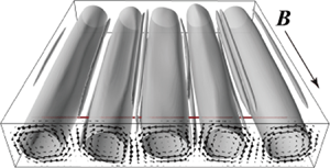
  $Q_{3D}$ value, the second invariant of the velocity gradient tensor calculated from the simulation results, displays convection rolls. A quasi-2-D shape of the rolls in the oscillatory condition provides evidence of 2-D oscillatory motion (figure 10a). We also calculated a spatio-temporal velocity map from the simulation results along a line corresponding to the present UV1 line measurement (
 $z = 0.25L$; dark red line in figure 10a). This map shows finer structures of the oscillatory convections (figure 10b). The corresponding mean velocity profile shown in figure 10(c) also has humps that reflect modifications of the main rolls. Figures 10(d)–10(f) show sequential snapshots of the vorticity field on a vertical cross-section of the fluid layer perpendicular to the magnetic field (
 $\omega _x$). Red and blue contours in the various panels represent positive and negative values of vorticity in the direction of the applied magnetic field (
 $x$-axis), respectively. The broken line in figure 10(d) indicates the measurement line corresponding to the ultrasonic transducer (figure 1). At the places corresponding to the humps, there is an additional recirculation vortex pair between the main rolls. The vortices seem to be a separation vortex pair from the main rolls and appear in between the roll flows detached from the wall, not approaching or adhering to the wall.

Figure 10. Results of numerical simulation performed for  $Ra = 1.0 \times 10^5$ and
  $Q = 3.2 \times 10^4$ (
 $Q/Ra = 0.32$). (a) The isosurface of
  $Q_{3D}$ represents the roll structures, where the dark red line indicates the place of the UV1 measurement line. (b) Spatio-temporal velocity map extracted along a line corresponding to the UV1 measurement line (see figure 1). (c) Time-averaged velocity profile of the velocity map. (d–f) Instantaneous contour maps of vorticity on the vertical cross-section at
  $x = 160\ \textrm {mm}$, where red and blue contours represent positive and negative values of the vorticity, respectively (see also supplementary movie 1).
Sequential snapshots shown in figure 10(d–f) also represent the motion of the rolls corresponding to the 2-D oscillations as a periodic distortion of the rolls into elliptic shapes. A remarkable feature of this distortion is that the roll axes are almost fixed at both horizontal and vertical positions. The distortion is accompanied by entraining the vorticity from the recirculation vortex pair; the entrainment occurs periodically and alternately between neighbouring main rolls, and deformation of the rolls behaves synchronously (see also supplementary movie 1 available at https://doi.org/10.1017/jfm.2020.1047). By the entrainment, the main rolls seem to be surrounded by an annular layer of opposite-sign vorticity. In this oscillation mode, fluid particles may follow an elliptic particle path in a  $y$–
$y$– $z$ cross-section different from the 3-D travelling wave oscillations. Along the periodic distortion, the cross-sectional area of the rolls periodically expands and shrinks similar to ‘breathing’. This behaviour of the rolls with rotation of the major axis of the elliptic shape is expressed by diagonal lines on the space–time velocity map (figure 10b). Similar diagonal stripe patterns are also observed in the velocity map measured by UVP (figure 4a). This supports the reliability of this numerical simulation.
No oscillatory convection is detected at  $Q > Q_{OS}(Ra)$, according to the present criteria. We investigated the mean velocity profile taken at this condition of the experiment to highlight the differences in the convection roll structures (figure 11). Here the profile was measured along UV1 at
  $Ra = 7.9 \times 10^4$ and
  $Q = 2.0 \times 10^5$ (
 $Q/Ra = 2.5$). The profile still has small but distinct humps and is asymmetric, representing elliptic main rolls with small recirculation vortex pairs. The corresponding r.m.s. values of the velocity fluctuations are small but significantly distributed. This condition therefore cannot be distinguished as a steady-state regime, even though a distinct peak frequency is not detected on the velocity fluctuation spectra. Under considerably smaller
  $Ra$ conditions, the velocity profile assumes a sinusoidal shape with horizontal symmetry in each roll. An example of these profiles is shown in figure 12 as the mean velocity profiles, where the original velocity data for the profile is from Vogt et al. (Reference Vogt, Ishimi, Yanagisawa, Tasaka, Sakuraba and Eckert2018) measured at
  $Ra = 1.7 \times 10^4$ and
  $Q = 8.0 \times 10^3$ (
 $Q/Ra = 0.47$) by UV2. Even in this condition, the profile of the r.m.s. value shows small, local maxima at the boundaries between the main rolls. A numerical simulation was also performed at similar parameters,
  $Ra = 1.4 \times 10^4$ and
  $Q = 5.7 \times 10^3$ (
 $Q/Ra = 0.41$), to determine the corresponding motion of the main rolls. A snapshot of the isosurface of the
  $Q_{3D}$ value also represents quasi-2-D rolls along the direction of the magnetic field (figure 13a).

Figure 11. Profiles of mean velocity  $U_y$ and standard deviation of velocity fluctuations
  $u_{y,rms}$ measured at
  $Ra = 7.9 \times 10^4$ and
  $Q = 2.0 \times 10^5$ (
 $Q/Ra = 2.5$) by UV1.

Figure 12. Profiles of mean velocity  $U_y$ and standard deviation of velocity fluctuations
  $u_{y,rms}$ using data from Vogt et al. (Reference Vogt, Ishimi, Yanagisawa, Tasaka, Sakuraba and Eckert2018) at
  $Ra = 1.7 \times 10^4$ and
  $Q = 8.0 \times 10^3$ (
 $Q/Ra = 0.47$) by UV2.

Figure 13. Results of numerical simulation performed for  $Ra = 1.4 \times 10^4$ and
  $Q = 5.7 \times 10^3$ (
 $Q/Ra = 0.41$). (a) Isosurface of the
  $Q_{3D}$ value representing roll structures, where the dark red line indicates the UV2 measurement line. (b) Spatio-temporal velocity map extracted along a line corresponding to the UV2 measurement line (figure 1). (c) Time-averaged velocity profile of the velocity map. (d,e) Instantaneous contour map of vorticity on the vertical cross-section at
  $x = 160\ \textrm {mm}$, where red and blue contours represent positive and negative values of the vorticity, respectively (see also supplementary movie 2).
The spatio-temporal velocity map shown in figure 13(b) extracted from the simulation results along the line corresponding to the UV2 measurement line (dark red line in figure 13a) displays longer-period periodic oscillation with substantially smaller amplitude than in the oscillations shown in figure 10(b). The mean velocity profile calculated from the map also has a quasi-sinusoidal shape with small deformation around the boundaries between the main rolls (figure 13c). Contour maps of the instantaneous vorticity field given from the simulation show the existence of small recirculation vortex pairs (figures 13d and 13e; see also supplementary movie 2). The numerical simulation elucidates that the vortex pair oscillates periodically and locally, and the distinct peaks of the r.m.s. values shown in figure 12 may represent such local oscillations. Such small vortex pairs and oscillations may not be distinguished by UVP measurements in the present experiment because of the arrangement of the measurement lines relative to the vortex pair and the inability to resolve small velocity fluctuations. The results summarized above suggest that there are two different types of 2-D oscillatory convection: weak and local oscillations on the recirculation vortex pair (corresponding to figures 11–13), and more dynamic and global elliptic oscillations of the main rolls accompanied by vorticity entrainment from the recirculation vortex pairs (figures 9 and 10).
Previous studies that assumed a wake of straight cylinders reported that such recirculation vortex pairs show absolute instability at relatively small Reynolds numbers,  $Re = O(10)$, and display periodic oscillations (e.g. Drazin & Reid Reference Drazin and Reid1998). With increasing
  $Re$ number,
  $O(10^2)$, the oscillations propagate from the recirculation vortex pair downstream. Here, unlike the wake, the main rolls are in tight interaction with the recirculation vortex pairs via vorticity entrainment and elliptic deformation of the roll in the 2-D oscillation with increasing velocity of the main rolls. In the next section, we investigate the convective flow velocity and dimensionless frequency of the oscillatory motion to characterize the 2-D oscillations.
3.5. Frequency and flow velocity on the 2-D oscillatory convection
This section discusses the characteristic frequency of the oscillatory convection  $f_{OS}$ and the local maximum value of the time-averaged velocity profile at the central convection rolls
  $U_{y,max}$ (figure 9), which are the basis for calculating the dimensionless frequency and
  $Re$ numbers. Variations in these values with respect to
  $Q$ are shown in figure 14. The
  $f_{OS}$ and
  $U_{y,max}$ values for the plots were obtained from spatio-temporal velocity maps measured by UV1 at different
  $Ra$ numbers for the five-roll state via the spatially averaged power spectrum of the velocity fluctuations and time-averaged velocity profile, respectively. The
  $f_{OS}$ detected by UV3 placed at the centre of the vessel parallel to UV1 are also plotted to evaluate the range of the 2-D oscillations in figure 14(a). The frequency gradually increases with decreasing
  $Q$ at all of the
  $Ra$ conditions studied here, with the largest increases observed for small
  $Q$ and the highest
  $Ra$ number of
  $Ra = 1.8 \times 10^5$. There is a very close coincidence of the
  $f_{OS}$ obtained by UV1 and UV3 at relatively large
  $Q$ values within the frequency resolution as expressed by the symbol overlap. At smaller
  $Q$, however, distinct peaks corresponding to
  $f_{OS}$ in UV3 cannot be distinguished and are buried in multiple peaks or noise, whereas the spectra obtained by UV1 show clear peaks. The coincidence suggests the existence of 2-D oscillations, whereas the disappearance may indicate a transition from the 2-D oscillatory convection regime to a 3-D flow regime. Vogt et al. (Reference Vogt, Ishimi, Yanagisawa, Tasaka, Sakuraba and Eckert2018) suggested that a transition from quasi-2-D convection to a 3-D flow regime appears as a meandering structure along the centreline of the vessel perpendicular to the magnetic field while fine structures move along the roll axis. The disappearance of a distinct peak in the spectra obtained by UV3 may reflect this; however, further detailed investigation is beyond the scope of the present study.

Figure 14. Variations of (a) the main frequency on the oscillatory convection,  $f_{OS}$, obtained by UV1 and UV3, and (b) the maximum time-averaged velocity of the central convection rolls,
  $U_{y,max}$, in the five-roll state with respect to
  $Q$ obtained at different
  $Ra$. In (a), the frequencies obtained by UV3 at most of the
  $Q$ values agree with those by UV1 within the frequency resolution as overlaps of the solid and open symbols.
The dependence of  $U_y$ on
  $Q$ shown in figure 14(b) is similar to the behaviour of the temperature oscillations in figure 7(a): the mean velocity initially slightly increases with decreasing magnetic field, reaches a maximum and then decreases. These observations can also be understood as growth of the 2-D oscillations and subsequent transition to a 3-D flow regime. At the opposite viewpoint,
  $U_{y,max}$ increases with increasing magnetic field strength in the range of small
  $Q$. This effect can likely be attributed to the stabilization and strengthening of the mean flow by the magnetic field. Burr & Müller (Reference Burr and Müller2002) reported an increase in heat transfer in RBC with the application of a horizontal magnetic field over a specific parameter range for Hartmann numbers
  $Ha = Q^{1/2} < 400$. As an explanation for the increase of flow transport properties, the authors suggested an enhancement of the quasi-2-D roll-type convection. A damping of the flow intensity occurs with further increases in
  $Q$ due to the emerging magnetic damping. This point is important in the discussion of flow transition and is further addressed in the following section.
The dimensionless frequency reduced by the circulation time (turnover time) of the main convection rolls,  $f^* = f_{OS}\tau _{TO}$, is plotted as a function of
  $Q/Ra$ in figure 15, where the circulation time is given as
  $\tau _{TO} = 2{\rm \pi} \Delta z/U_{y,max}$, with the displacement of the measurement line from the centre of the rolls,
  $\Delta z = 10\ \textrm {mm}$ (figure 1). At sufficiently high magnetic fields (
 $Q/Ra \gtrsim 0.3$) the values obtained by UV1 and UV3 collapse into a unified curve (i.e. the symbols overlap) and
  $f^*$ assumes a nearly constant value around 0.6. The supplemental numerical simulations shown in figures 10 and 13 provide a similar dimensionless frequency,
  $f^* \sim 0.6$. As mentioned, the finding of a consistent and constant dimensionless frequency can be interpreted as an indication of a 2-D flow structure, whereas the scattering of the data for
  $Q/Ra \lesssim 0.3$ can be understood as the transition from the 2-D oscillatory convection regime to a 3-D flow regime. The transition point at
  $Q/Ra \approx 0.3$ corresponds to the one at which the r.m.s. value of the temperature fluctuation,
  $T_{rms}$, reaches the maximum (figure 7b). Furthermore, the
  $Re$ number also reaches a maximum here as discussed in § 4.1. Together these results indicate that the decrease in
  $T_{rms}$ and flow velocity are both caused by the transition to a 3-D flow regime and that the transition can be organized by
  $Ra/Q$.

Figure 15. Dimensionless frequencies determined by UV1 and UV3 plotted at different  $Ra$ versus
  $Q/Ra$, where the frequencies obtained by UV3 at most of the
  $Q/Ra$ values agree with those by UV1 within the frequency resolution as overlaps of the solid and open symbols. There exist no symbols for UV3 for small
  $Q/Ra$ values because of unclear frequencies by UV3.
4. Discussion
The experimental and numerical results shown in the previous section indicate that the 2-D oscillatory convection accompanies oscillations of the recirculation vortex pairs situated between the main rolls, and that there are two different types of oscillations. The recirculation vortices play an important role in the onset of instabilities, which is deduced to be dominated by the inertia of the flow from the knowledge of absolute instability of the wake. Here we discuss the physics behind the variations in the  $Re$ number of quasi-2-D flows and its relation to the fraction of
  $Q/Ra$ with arguments based on MHD for a unified understanding of the involved phenomena.
4.1. Variation of the Reynolds number
In the case of quasi-2-D convection consisting of parallel convection rolls, we use the velocity in the rolls,  $U_{y,max}$, and the vessel height,
  $L$, to define the Reynolds number as
  $Re_{2D} = U_{y,max}L/\nu$. The variation of
  $Re_{2D}$ with
  $Q$ obtained at different
  $Ra$ values for the five- and six-roll states are plotted in figure 16(a,b), respectively. Larger open symbols (and grey crosses) indicate
  $Re_{2D}$ values corresponding to the critical value of the Chandrasekhar number for the onset of the oscillations
  $Q_{OS}$ shown in figure 6;
  $Q_{OS}$ here indicates the onset of more dynamic 2-D oscillations discussed in § 3.4 and is determined along the criteria mentioned in § 3.2. For the range of
  $Ra$ numbers considered here, the oscillations occur for
  $Re_{2D} > 800$. It can be assumed that the flow velocities in the main convection rolls are sufficiently large in this range to entrain the vorticity from the recirculation vortex pair to form dynamic 2-D oscillations. A re-examination of data published in our previous papers (Tasaka et al. Reference Tasaka, Igaki, Yanagisawa, Vogt, Zuerner and Eckert2016; Vogt et al. Reference Vogt, Ishimi, Yanagisawa, Tasaka, Sakuraba and Eckert2018) also indicates that for
  $Q > 10^3$ the steady conditions maintain
  $Re_{2D} < 800$ and the first oscillation of five or six rolls appears at
  $Re_{2D} > 800$. Here, the value 800 of the
  $Re$ number itself probably has no universal character and may change depending on the vessel aspect ratio, as discussed later.

Figure 16. Variations in Reynolds numbers for quasi-2-D flows,  $Re_{2D}$, plotted with decreasing
  $Q$ at different
  $Ra$ values and different number of rolls: (a)
  $n = 5$ and (b)
  $n = 6$, respectively. The grey lines are guides for variations proportional to
  $Q^{-0.2}$ and
  $Q^{-0.5}$; larger open symbols (grey cross symbols) indicate
  $Re_{2D}$ values corresponding to
  $Q_{OS}$ in figure 6. Coloured broken lines indicate approximations of the variations of
  $Re_{2D}$ considering the influence of
  $Q$ on the critical
  $Ra$ at the onset of convection,
  $Ra_{c}(Q)$. The constant 250 is set empirically.
The log–log plot in figure 16 indicates that the main part of the dependence of  $Re$ on
  $Q$ cannot be described by a single power law as shown by the grey auxiliary lines in the figure representing the slopes of
  $Re_{2D} \propto Q^{-0.2}$ and
  $\propto Q^{-0.5}$; the variations seem to be steeper with respect to
  $Q$. Notably, there is a maximum in the
  $Re$ number as in the temperature fluctuations (figure 7), especially in the case of large
  $Ra$. The reduction of
  $Re_{2D}$ in the case of small
  $Q$ may be accompanied by the transition to a 3-D flow regime, whereas the decrease in flow amplitude at high
  $Q$ may be due to the Hartmann braking effect.
4.2. Scaling for variations of Reynolds numbers
Here we consider the scaling law of  $Re_{2D}$ to cover a wide range of the variations shown in figure 16. To describe the variation in
  $Re_{2D}$ where the slope gradually changes with
  $Q$, we express the effect of magnetic damping using the critical Rayleigh number for the onset of convection as a function of
  $Q$. The key phenomenon to evaluate the magnetic damping is the Hartmann braking in the boundary layer formed on the walls perpendicular to the magnetic field (Hartmann layer, figure 17). Burr & Müller (Reference Burr and Müller2002) explained Hartmann braking in the present system as follows:

Figure 17. Schematic drawing of the Hartmann layer formed near a sidewall parallel to the magnetic field: (a) with convection rolls and (b) with contours of the induced electric currents displayed on the midplane.
In the core region the Lorenz forces are directed opposite to the convective motions whereas at the Hartmann walls their direction is reversed and the fluid is accelerated. This renders the Hartmann layers very thin and thereby, together with conducting Hartmann walls, they govern the current density and with it the damping of velocity in the core region. The energy removed from the core region is dissipated by Joule dissipation in the Hartmann walls and by Joule and viscous dissipation in the Hartmann layers.
In the present system, an electrically insulating material is used as the sidewalls and thus the energy dissipation occurs in the Hartmann layer. With increasing  $Q$, the Hartmann layer becomes thinner and viscous dissipation becomes stronger. In the results of linear stability analysis performed by Burr & Müller (Reference Burr and Müller2002), the critical
  $Ra$ number for the onset of convection with regard to Hartmann braking,
  $Ra_{c}(Q)$, was given as a relation of
  $Ra_{c}$ versus
  $1/\tau _{m}$ (figure 18). The time scale of magnetic damping by the Hartmann braking,
  $\tau _{m}$, is given from (22) in Burr & Müller (Reference Burr and Müller2002) as
 \begin{equation} \frac{1}{\tau_{m}} = \frac{Q^{1/2}}{b} + \frac{Qc_{H}}{b+c_{H}}, \end{equation}
where  $b$ and
  $c_{H}$ denote the dimensionless half-width of the fluid layer parallel to the magnetic field and the electrical conductivity of the sidewall, respectively.

Figure 18. Neutral stability curve for the onset of convection replotted from Burr & Müller (Reference Burr and Müller2002). The top axis represents the corresponding Chandrasekhar number  $Q$ for
  $c_{H}$ = 0 and
  $b = 2.5$ calculated from magnetic damping time
  $\tau _{m}$ in (22) of Burr & Müller (Reference Burr and Müller2002), where the arrow indicates the range of
  $Q$ examined in the present study.
The Prandtl free-fall velocity for thermal convection indicates that the representative velocity  $W_0$ is
  $W_0 \sim \sqrt {g\beta \Delta TL}$. This makes the
  $Re$ number for the case of non-magnetic field approximately
  $Re \sim (Ra/Pr)^{1/2}$. By extending this relation, the variations in
  $Re$ number can be expressed as
 \begin{equation} Re_Q \sim \left[\frac{Ra}{Pr}\frac{Ra_c(Q=0)}{Ra_c(Q)} \right]^{1/2} = A \left[ \frac{Ra}{Ra_{c}(Q)} \right]^{1/2}\quad (\text{with $A$ a coefficient constant}), \end{equation}
where the inertia generated by buoyancy is given as a value of  $Ra$ relative to
  $Ra_{c}(Q)$. We revisit figure 16 to evaluate the applicability of the present scaling law derived above. The dimensionless half-length is
  $b = 2.5$ and the sidewalls are electrically insulated (
 $c_{H} = 0$). The
  $Ra_{c}$–
 $Q$ dataset was formed (figure 18) by reading off
  $Ra_{c}$–
 $1/\tau _{m}$ in Burr & Müller (Reference Burr and Müller2002). Variations of
  $Re_Q$ are thus calculated from the dataset at different
  $Ra$ numbers, as shown by dashed lines in figure 16, where the coefficient
  $A = 250$ was empirically determined to fit the result for the five-roll state (
 $n = 5$) at
  $Ra = 7.9 \times 10^4$. This value is very close to
  $[Ra_c(Q=0)/Pr]^{1/2} = (1708/0.03)^{1/2} \approx 239$ in (4.2). The variations of
  $Re_{2D}$ can be approximated by the present scaling law of (4.2) in the moderate
  $Q$ range depending on
  $Ra$. This suggests that the convection velocity is determined by the effective
  $Ra$ numbers, i.e. distance from the neutral stability curve under a horizontal magnetic field. The critical Chandrasekhar numbers,
  $Q_{OS}$, for the onset of 2-D oscillations appear to occur at which the present
  $Re_{2D}$ data fail to match the present scaling law for large Q. The data also deviate from the scaling law for small
  $Q$, which arises from the transition to a 3-D flow regime discussed in the previous section.
4.3. Scaling in the steady 2-D regime
Variations in  $Re_{2D}$ appear steeper and detach from the scaling law of (4.2) for relatively large
  $Q$ values (figure 16). At sufficiently large
  $Q$, 2-D oscillatory convection may be suppressed into steady 2-D convection. The scaling law describing the steeper slope may thus be derived to consider the condition. The influence of viscous dissipation can be disregarded in cases of sufficiently large
  $Ra$ and
  $Q$, and the equation of motion for the vertical velocity
  $w$ in the quasi-2-D flows is reduced to
 \begin{equation} \frac{\textrm{D}w}{\textrm{D}t} \sim F_{b} - F_{H}, \end{equation}
where  $\textrm {D}/\textrm {D}t$ is a material derivative, and the force terms on the right-hand side are the buoyancy and the magnetic damping by Hartmann braking. The order of (4.3) is evaluated using the characteristic velocity
  $W$ with the time scale of Hartmann braking
  $\tau _{H}$ as
 \begin{equation} \frac{\textrm{D}W}{\textrm{D}t} \sim g\beta \Delta T - \frac{W}{\tau_{H}}. \end{equation}
 From Sommeria & Moreau (Reference Sommeria and Moreau1982), the dissipation time scale of the Hartmann braking is given as  $\tau _{H} = (a/2B)(\rho/\sigma \nu)^{1/2}$ with the spacing between walls
  $a$. The expression of
  $\tau _{H}$ is equivalent to
  $\tau _{m}$ in (4.1) for
  $c_{H} = 0$. Here we reformulate the time scale using length scale
  $L$ as
 \begin{equation} \frac{1}{\tau_{H}} \sim \frac{Q^{1/2}}{b}\frac{\nu}{L^2}. \end{equation}
This includes the dimensionless half-width  $b$ (= 2.5), whereas the thickness of the Hartmann layer,
 \begin{equation} \delta_{H} \sim Q^{-1/2}L, \end{equation}
is independent of  $b$.
$b$.
It is assumed that the fluid flow is in steady condition with  $Q$ larger than the critical Chandrasekhar number
  $Q_{OS}(Ra)$ for the onset of 2-D oscillations. Equilibrium velocity
  $W^*$ in the condition is thus determined by the balance between the buoyancy and the magnetic damping by Hartmann braking. Following the procedure to evaluate convection velocity considering magnetic damping in Davidson (Reference Davidson2017, § 6.2.5), (4.4) is simplified by substituting (4.5):
 \begin{equation} \left. \begin{gathered} g\beta \Delta T = \frac{W^*}{\tau_{H}}, \\ Ra\frac{\kappa\nu}{L^3} = W^*\frac{Q^{1/2}}{b}\frac{\nu}{L^2},\\ W^* = \frac{Ra}{Q^{1/2}}\frac{\kappa}{L}b. \end{gathered} \right\} \end{equation}
The  $Re$ number for steady quasi-2-D flows becomes
 \begin{equation} Re_{2D} = \frac{W^*L}{\nu} \sim \frac{Ra}{Q^{1/2}}\frac{b}{Pr}. \end{equation}
Equation (4.8) indicates that the variations in  $Re_{2D}$ depend on
  $Q$ with an exponent of
  $-1/2$ for the limiting case that inertia can be neglected compared with the electromagnetic forces, here
  $Q > 10^5$ in figure 16. Using Prandtl free-fall theory for a non-magnetic field,
  $Re \sim (Ra/Pr)^{1/2}$, the relative
  $Re$ number under magnetic field to this
  $Re$ becomes
 \begin{equation} \frac{Re_{2D}}{Re} \sim \left(\frac{Ra}{Q}\right)^{1/2} \frac{b}{Pr^{1/2}}. \end{equation}
 Variations in  $Re_{2D}$ reduced by
  $Ra^{1/2}$ are shown in figure 19, where
  $Q$ in the abscissa is also reduced by
  $Ra$. The curve representing the power law derived above is indicated by a broken line. The data collapse reasonably well into a unified curve and the variations of
  $Re$ seem to approach the slope of the broken line for larger
  $Q$,
$Q$,  $Q/Ra \gtrsim 1$. It can be speculated that, if
  $Q / Ra$ values decrease, the data deviate from this power law after the 2-D oscillations have appeared. The power law based on the assumption of the balance between the buoyancy and the magnetic damping by Hartmann braking is not valid at weaker magnetic fields where inertia must be taken into account.

Figure 19. Values of  $Re_{2D}$ as a function of
  $Q/Ra$ for different
  $Ra$ conditions reduced by
  $Ra^{0.5}$ according to the scaling law: (a)
  $n = 5$ and (b)
  $n = 6$. Larger open symbols (grey cross symbols) indicate
  $Re_{2D}$ values corresponding to
  $Q_{OS}$ in figure 6.
The applicability of the criterion that the present power law of  $Re_Q$ determines the onset of 2-D oscillation is now evaluated for the previous results obtained with
  $Q/Ra < 1$. The regime diagram summarized in Vogt et al. (Reference Vogt, Ishimi, Yanagisawa, Tasaka, Sakuraba and Eckert2018) is shown in figure 20 with the critical Chandrasekhar number
  $Q_{OS}$ obtained in this study, where square and diamond symbols indicate the steady and the 2-D oscillation regimes with five or six rolls, respectively. The red line in figure 20 represents the contour
  $Re_Q = 250[Ra/Ra_{c}(Q)]^{1/2} = 800$, where
  $Re_{2D} = 800$ is chosen as the lower limit at which the 2-D oscillation emerges (figure 16). The line is a good approximation of the border between the steady and the 2-D oscillation regimes.

Figure 20. Critical Chandrasekhar number  $Q_{OS}$ for different
  $Ra$ values (figure 6) plotted on the regime diagram provided by Vogt et al. (Reference Vogt, Ishimi, Yanagisawa, Tasaka, Sakuraba and Eckert2018), where broken black lines indicate contours of
  $Ra/Q$. The solid black line shows critical Rayleigh numbers for the onset of convection calculated from the results of Burr & Müller (Reference Burr and Müller2002) with
  $b = 2.5$. The red line represents the contour line of
  $Re_Q = 250[Ra/Ra_{c}(Q)]^{1/2} = 800$ as the proposed critical condition of quasi-2-D oscillations for cases of
  $Q/Ra \lesssim 1$.
Through a detailed investigation of the results obtained here and following the above discussion, the flow regimes may be dominated by a  $Re$ number determined by the distance from the neutral stability curve (black solid line in figures 18 and 20). The fraction
  $Q/Ra$ appears as the dominant factor that determines the regimes in conjunction with
  $Re$, e.g.
  $Q/Ra \approx 1$ for the onset of dynamic oscillation, and
  $Q/Ra \approx 0.3$ for the transition to a 3-D flow regime. These conditions of the fraction, however, are given for the specific value of
  $b\ (= 2.5)$. It is thus trivial that the fraction may not be a universal factor to describe the phenomena, and the condition
  $Q/Ra \approx 1$ for the onset of dynamic oscillation is modified by different
  $b$ values.
4.4. Relation to previous studies
According to the derivation process of the scaling law in (4.9), the  $Re$ number strongly depends on the half-length of the fluid layer (
 $b$ in (4.9)) in the direction of the magnetic field because of the dominance of Hartmann braking on the fluid layer. The fluid layer used in Burr & Müller (Reference Burr and Müller2002) has a larger
  $b = 5$, compared with
  $b = 2.5$ in the present set-up (figure 17). The differences in the critical conditions for the onset of oscillatory convection in their results show substantially smaller critical
  $Ra$ numbers than the present results, which can be explained by a further discussion of reasons below. Here we assume that the flow regimes are dominated by the
  $Re$ number according to the previous discussions. Fluid layers of larger horizontal extents in the direction of the magnetic field would achieve sufficiently large
  $Re$ numbers for the transitions even with smaller
  $Ra$, at similar
  $Q$ conditions to those in the present study. This is because of the reduced influence of Hartmann braking on the variations of
  $Re$. There are also differences in the criterion determining the onset of oscillation. Burr & Müller (Reference Burr and Müller2002) used the temperature fluctuation intensity measured at the central part of the fluid layer, whereas we determined the investigated frequency component
  $f = f_{OS}$ of the velocity fluctuations at which the r.m.s. value reaches the local maximum in the profile. As mentioned in § 3.4, there are two different types of 2-D oscillatory convection: weak and local oscillations of the recirculation vortex pair between the main rolls, and more dynamic and global elliptic oscillations of the main rolls accompanying vorticity entrainment from the recirculation vortex pair. From these observations it is suggested that Burr & Müller (Reference Burr and Müller2002) detected the former, whereas the present study investigated the latter.
The flow development and transitions dominated by Hartmann braking are not a specific problem in this study, but are common characteristics that influence low-magnetic-Reynolds-number flows confined by walls of electrically insulating materials. Knaepen & Moreau (Reference Knaepen and Moreau2008) predicted that MHD damping in the flows confined by walls perpendicular to the magnetic field is not characterized by the interaction parameter  $N = Q/Re$, but by
  $Ha/Re$ (or
  $N/Ha$ in a different form; see also Sommeria & Moreau (Reference Sommeria and Moreau1982) and Moreau, Thess & Tsinober (Reference Moreau, Thess and Tsinober2007)). In the present system,
  $Ha/Re$ is modified to
  $(QPr/Ra)^{1/2}$ as
  $Re \propto (Ra/Pr)^{1/2}$. This prediction agrees with the results obtained here. It may thus be concluded that the present results provide experimental evidence for this prediction.
5. Concluding remarks
We investigated 2-D oscillatory motions on quasi-2-D convection rolls that have been reported in Rayleigh–Bénard convection with an imposed horizontal magnetic field at relatively large Rayleigh-number  $Ra$ and Chandrasekhar-number
  $Q$ conditions. The investigation was performed by considering the morphology, generation and mechanism that give rise to the oscillations through laboratory experiments using eutectic GaInSn as the test fluid filling in a vessel with an aspect ratio of five. Supplemental numerical simulations were performed to determine the details of the flow structures. Multi-line measurements of the instantaneous velocity profiles performed by ultrasonic velocity profiling at conditions of
  $7.9 \times 10^4 \le Ra \le 1.8 \times 10^5$ and
  $2.5 \times 10^4 \le Q \le 1.9 \times 10^5$ and the numerical simulations elucidated the emergence of two different types of 2-D oscillations. One is dynamic and global oscillations accompanied by vorticity entrainment from recirculation vortex pairing of separation flows detaching from the walls between neighbouring main rolls. The other is weak localized oscillations of the vortex pair. The source of the oscillations was found to lie in the periodic oscillations of the recirculation vortex pair. Despite different
  $Ra$ conditions, the oscillations occur at similar Reynolds numbers (
 $Re_{2D} > 800$). These
  $Re_{2D}$ values are sufficiently large to cause oscillatory instability in the recirculation vortex pairs. This is considerably different from the 3-D travelling wave propagation along the roll axis predicted by stability analysis at relatively small
  $Q$ conditions,
  $Q = O(10)$, as enlargements of the Busse balloon. The 2-D oscillations are caused by sufficiently high inertia provided by the large
  $Ra$ and 2-D restrictions. The intensity of the temperature fluctuations and Reynolds number
  $Re_{2D}$ increase with decreasing
  $Q$, along with the development of 2-D oscillations, and further decrease with decreasing
  $Q$ because of a transition from the 2-D oscillation regime to a 3-D flow regime.
A scaling law describing the variation of  $Re_{2D}$ was derived with an effective
  $Ra$ number reduced by a critical
  $Ra$ number as a function of
  $Q$ as
  $Re_Q \propto [Ra/Ra_{c}(Q)]^{1/2}$. The contour of
  $Re_Q = 800$ given from the scaling law shows good agreement with the boundaries of oscillatory and steady-state regimes obtained in previous experiments under relatively small
  $Q$ conditions. A considerably steeper decrease of
  $Re_{2D}$ around the onset of the 2-D oscillations for relatively large
  $Q$ seems to approach
  $(Q/Ra)^{-1/2}$. This corresponds to the scaling law derived from the assumption of a balance between buoyancy and magnetic damping by Hartmann braking near the sidewall of the vessel perpendicular to the magnetic field in the steady regime. These results suggest that the emergence of 2-D oscillatory convection is governed by the competition between the buoyancy in the core region and viscous dissipation in the thin Hartmann layer, and therefore its onset is determined by
  $Re_{2D}$.
Supplementary movies
Supplementary movies are available at https://doi.org/10.1017/jfm.2020.1047.
Acknowledgements
Numerical simulations were performed on the Earth Simulator at JAMSTEC.
Funding
This work was supported by JSPS KAKENHI grant no. 24244073. The activities of Y.T. at Helmholtz Zentrum Dresden-Rossendorf (HZDR) were supported by JSPS KAKENHI grant no. 15KK01219. The authors acknowledge Dr S. Eckert and Dr T. Vogt in HZDR for their technical support in the experiments and fruitful discussions.
Declaration of interests
The authors report no conflict of interest.


