


1. Introduction
Industrial processes dealing with micro-object manipulation mainly use vacuum (suction) as a handling principle. However, at microscale (typically below 1 mm), these processes reach some limitations. Physically, these limitations are primarily due to adhesion forces interfering with vacuum (van der Waals, electrostatic, etc.) that are, indeed, no more negligible at these scales (Lambert et al. Reference Lambert, Borno, Lendersand, Malharbizand, Mastrangeli, Ondarçuhu, Takei, Valsamis and De Volder2013). And technically, the reliability of the assembly is limited by the positioning precision of the actuators.
One way to overcome adhesion and positioning issues at the same time would be to use capillary forces as a gripping principle. Previous research has evidenced that it was possible to tune these forces and to take advantage of them in order to facilitate microassembly and microgripping processes. A recent work by Iazzolino et al. (Reference Iazzolino, Tourtit, Chafaï, Gilet, Lambert and Tadrist2020) reviews the proofs of concept for capillary gripping tools or capillary self-assembly processes. Without aiming to be exhaustive on the technical capillary handling and assembly solutions, we may, however, give a few examples. Some of these capillary grippers are based on water condensation and temperature variations (Uran, Safaric & Bratina Reference Uran, Safaric and Bratina2017), on laser evaporation and changes in the contact conformity (Iazzolino et al. Reference Iazzolino, Tourtit, Chafaï, Gilet, Lambert and Tadrist2020), variation of wettability (Fantoni, Hansen & Santochi Reference Fantoni, Hansen and Santochi2013), on liquid volume control through 3-D printed and replicated microchannels (Dehaeck et al. Reference Dehaeck, Cavaiani, Chafai, Tourtit, Vitry and Lambert2019), or finally based on electrowetting as introduced by Apoorva, Maccurdy & Lipson (Reference Apoorva, Maccurdy and Lipson2014) and Vasudev et al. (Reference Vasudev, Jagtiani, Du and Zhe2009). High-speed self-assembly lines using capillary forces are presented by Knuesel & Jacobs (Reference Knuesel and Jacobs2010) and Park et al. (Reference Park, Fang, Biswas, Mozafari, Stauden and Jacobs2015).
Capillary forces are generated by a liquid meniscus binding a substrate (e.g. a circuit card or a gripper) and the object to assemble or to handle. One crucial phenomenon occurring in this case is the self-alignment effect. It consists of a passive alignment motion centring the component with respect to the substrate, and coming to a stop when the state of minimum energy is reached in the system.
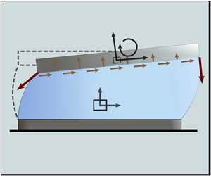
This paper focuses on the modelling of the capillary self-alignment process. Prior models have aimed at describing the modes of deformation of menisci either in statics or in dynamics. These six modes of deformation are presented in figure 1(a). Translational movements along the horizontal axis are called shifts, while those along the vertical axes are named lifts. Rotations around horizontal and vertical axes are called tilts and twists, respectively.

Figure 1. Usual terminology used in capillary gripping and self-assembly fields. (a) Modes of deformation of a liquid meniscus bounding two solid objects; (b) one-dimensional (1-D) uncoupled model for the shift where the 1-D linear fluid velocity distribution is described as  $\boldsymbol {v}_x=\dot {x}z/h \, \boldsymbol {1}_x$; (c) 1-D coupled model for the shift where
  $\boldsymbol {v}_x=f(t,z) \, \boldsymbol {1}_x$; (d) two-dimensional (2-D) coupled model for shift, tilt, lift with a two degrees of freedom (2-DOF) fluid,
  $\boldsymbol {v}_x$ and
  $\boldsymbol {v}_z$.
Models of liquid flows between two planes have been reviewed by Engmann, Servais & Burbidge (Reference Engmann, Servais and Burbidge2005). Several boundary conditions for the fluid velocity are considered (i.e. perfect and partial slip or no-slip boundary conditions). In the presented models, deformations and stresses inside the liquid meniscus are mathematically described.
Concerning static descriptions of the self-alignment, the twist motion has been studied by Takei, Matsumoto & Shimoyama (Reference Takei, Matsumoto and Shimoyama2010) where the capillary torque is measured for validation thanks to an experimental set-up using a magnetic field in which the specific micro-object behaves like a compass. A quasi-static axisymmetric 2-D study is presented by Mastrangeli et al. (Reference Mastrangeli, Valsamis, Van Hoof, Celis and Lambert2010), in which a finite element model based on the Surface Evolver software (Brakke Reference Brakke1992) and one analytical energy minimisation model are presented. The validation relies on a force measurement experiment where the bottom pad is mechanically shifted and the top pad is linked to two parallel cantilevers acting as a spring. This way, this system provides a specific kinematics, where the top pad is forced to move only by shifting, and without tilting. Mastrangeli et al. (Reference Mastrangeli, Valsamis, Van Hoof, Celis and Lambert2010) highlight the self-alignment hysteresis for large shifts. The shifts, tilts, lift and twist modes of deformations are further considered for square pads (Berthier et al. Reference Berthier, Brakke, Grossi, Sanchez and Di Cioccio2010), while Berthier et al. (Reference Berthier, Mermoz, Brakke, Sanchez, Frétigny and Di Cioccio2013) focus on shifts for more complex geometries. The stability of the tilt is studied in a different configuration by Berthier et al. (Reference Berthier, Brakke, Mermoz, Frétigny and Di Cioccio2015) with hydrophilic bands to increase the stabilisation of the square pads on the substrate. A model for capillary forces where a square pad is linked by a droplet of glue has been developed by Lienemann et al. (Reference Lienemann, Greiner, Korvink, Xiong, Hanein and Böhringer2003). The Surface Evolver software is used to get the geometry of the glue meniscus and coupled to ANSYS to get its elastic properties. The model has been used to investigate the influence of surface defects and self-assembly processes optimisation.
Papers studying self-alignment effects are also found in the specific literature of packaging. There, the self-alignment motion of the chip is induced by the surface tension of the solder joints. Goldmann (Reference Goldmann1993) introduces an equation linking the lift motion to the force applied on the upper cylindrical pad. This axisymmetric model is valid for deformations up to  $10\,\%$ of the zero-loaded meniscus height. Patra & Lee (Reference Patra and Lee1991) present a three-dimensional (3-D) quasi-static model for cylindrical pads, based on the surface energy minimisation, and taking no tilt and twist motions into account. A 3-D volume of fluid (VOF) modelling is investigated by Najib et al. (Reference Najib, Abdullah, Saad, Samsudin and Che Ani2017), where the authors focus on the self-assembly of surface mounted components. As the fluid is here a solder paste, the equations modelling the situation are coupled with the heat equation, and solved together in Fluent. Validation of the transient state is not documented in detail but the steady state shows a good agreement with experimental data.
First dynamical models have been developed by Meurisse & Querry (Reference Meurisse and Querry2006) and van Veen (Reference van Veen1999). The latter presents an analytical solution for independent lift and shift motions. The lift motion derives from Newton's equation, where the spring force is obtained from the surface energy minimisation method. The friction force in the liquid meniscus arises from the rheology literature and in particular Stefan's adhesion equation, which describes the normal viscous force acting between two disks being separated or brought closer. For the shift motion, the height of the liquid meniscus is considered to be constant. For the viscous friction force, the liquid velocity is modelled as in the steady state fluid flow with a linear distribution. This situation corresponds to figure 1(b). The axial and lateral motions of the micro-object are therefore the solution of second-order linear ordinary differential equations. But because the period of the oscillations can be smaller than the time required to reach the steady state, as shown by Lu & Bailey (Reference Lu and Bailey2005), it is necessary to couple the mechanical and fluid physics to describe the self-alignment process in a more accurate way. A model considering such a velocity distribution (see figure 1c) is introduced by Lu & Bailey (Reference Lu and Bailey2005). In this model, Surface Evolver is used to compute the force applied by the liquid on the object. The speed and displacement of the latter are computed and used in order to get the flow velocity distribution for the considered time step by solving coupled Newton and Navier–Stokes equations with the software Physica. Kaneda et al. (Reference Kaneda, Yamamoto, Nakaso, Yamamoto and Fukai2007) present a dynamical model for the tilt and lift motions. This model predicts the oscillatory characteristics of the system and the shape of the meniscus by solving Newton's equations for viscous and capillary forces applied on the solid structure. The shape of the meniscus is obtained thanks to geometrical and volume conservation assumptions. This transient 2-D modelling of a 1-DOF circular pad describes one out of two tilt motions. A 2-D model (see figure 1d) based on the VOF method is studied by Lin et al. (Reference Lin, Tseng and Kan2009). There, the chip is not totally wetted as the meniscus is pinned because of hydrophobic areas on the chip and the substrate. Lambert et al. (Reference Lambert, Mastrangeli, Valsamis and Degrez2010) report a semianalytical solution using the Chebyshev spectral method to solve his coupled 1-D system of equations describing the physics, therefore providing an analytical solution for a 1-DOF shifting chip. For the lift degree of freedom, a model based on a Kelvin–Voigt material (setting a spring, a mass and a damper in parallel) is presented by Valsamis et al. (Reference Valsamis, Mastrangeli and Lambert2013). The stiffness, damping coefficient and the mass are analytically expressed. The model is simulated with COMSOL Multiphysics while harmonic response tests are performed for the validation. This axisymmetric model describing the lift motion applies to cylindrical chips. Table 1 gives an overview of these different dynamical models with additional information.
Table 1. Overview of the dynamical self-alignment models and their experimental validations. The terms ‘1-D uncoupled’, ‘1-D coupled’ and ‘2-D coupled’ refer to figure 1(b–d), respectively. The following abbreviations are used: rectangular (Rect.); finite element method (FEM).

In this paper, our different models, which all derive from one another with successive simplifying assumptions, will first be introduced and the experimental validation set-up will then be presented. Our models aim at describing the transient damped oscillatory motion of self-alignment that would be encountered in the capillary microgripping or microassembly fields.
Here, the arbitrary Lagrangian–Eulerian (ALE) method used to numerically solve the general description of the coupled self-alignment effect (model 1) and the spherical caps assumption for the 3-DOF modal analysis (models 2 and 3) are new and specific to this paper. The semianalytical equations obtained in models 3 and 4 are original ways to solve this coupled problem.
In these models, handled objects are submillimetre rectangular chips with sharp edges. Considering a capillary gripping or self-assembly system, the liquid binding the chip to its substrate would be pinned on these edges. Because of these context requirements, our models must thereby give a transient description of the physics and take the geometrical pinning of the meniscus and the rectangular shape of the chip into account.
Eventually, the results from modelling and experimental tests will be compared (in terms of period of oscillation and damping constant) by changing the volume of the liquid layer. These results are finally discussed.
2. Self-alignment models
Models presented in this paper all consider the motion of a rectangular chip linked by a liquid meniscus to a rectangular substrate.
Figure 2 presents the configuration and the supplementary material defines the notations used in the following 2-D models. There, points  $P$ and
  $Q$ represent left- and right-hand edges in the
  $\boldsymbol {1}_y$ direction. In three dimensions, the length of these edges would be
  $D$. Angles
  $\phi +\varTheta _P$ and
  $\psi -\varTheta _Q$ are defining the direction of the force acting on the triple line during the motion. The height of the solid pad in motion at abscissa
  $x$ and at time
  $t$ is given by
  $H(x,t)$. The liquid meniscus is assumed to be pinned on the edges of the chip and substrate (i.e. at points
  $P$,
$P$,  $S_P$,
  $Q$ and
  $S_Q$). The shift, tilt and lift motions of the chip are computed by solving these models, while the twist motion is not considered in this work. Note that not all the notations are used in each model.

Figure 2. Illustration of 2-D self-alignment motion of a rectangular pad linked to a similarly shaped substrate by a liquid meniscus. The grey dashed lines sketch the rest state of the system. Here  $\boldsymbol {F}_{T_P}$ and
  $\boldsymbol {F}_{T_Q}$ are the tension forces applied on the triple line interface,
  $P_g$ is the ambient pressure and point
  $G$ is the centre of mass of the rectangular pad. Its coordinates along
  $\boldsymbol {1}_x$ and
  $\boldsymbol {1}_z$ are the shift and lift DOF. Here
  $\theta$ (the tilt) is the third degree of freedom of the pad. The meniscus, respectively, forms the angles
  $\phi +\varTheta _P$ and
  $\psi -\varTheta _Q$ at points
  $P$ and
  $Q$ with the vertical axis. Angles
  $\varTheta _P$ and
  $\varTheta _Q$ expressed as functions of the DOF
  $x_G$,
  $z_G$ and
  $\theta$ can be found in appendix B. These two angles are positive when the solid shifts rightwards.
2.1. Fully numerical 2-D nonlinear model
The model presented in this section is the most general of the four models presented here and allows nonlinearities for the coupled solid and fluid physics. The stresses are computed in the solid pad domain. The equations used in this model are numerically solved in the software COMSOL Multiphysics and rely on references COMSOL (2017) and COMSOL (2018).
The model consists of a meshed solid domain (i.e. the pad) and a meshed fluid domain (the liquid meniscus). The substrate is included in the model as a boundary and is not meshed. Considering that Eulerian and Lagrangian descriptions (for the fluid and the solid physics, respectively) are mixed in this model, the ALE method (Donea et al. Reference Donea, Huerta, Ponthot and Rodriguez-Ferran2017) is used to combine these descriptions in the following developments. In both domains, the Laplace equation  $\nabla ^{2} \boldsymbol {u}_{{mesh}} = 0$ is solved to spread the deformation of the mesh. The mesh displacement vector is given by
  $\boldsymbol {u}_{{mesh}}$ (m).
2.1.1. Physical description of the liquid meniscus
As sketched in figure 2, in this numerically solved model, we consider a liquid meniscus pinned on the edges of a solid pad on one side, and of a substrate on the other side. The liquid is considered incompressible. The viscous dissipation and inertial effects are likely to be significant. Therefore, the velocity and pressure fields in the meniscus are obtained by solving the isothermal Navier–Stokes equations for an incompressible fluid
 \begin{gather} \rho\frac{\partial \boldsymbol{v}}{\partial t} + \rho\left(\left( \boldsymbol{v}-\frac{\partial \boldsymbol{u}_{{mesh}}}{\partial t}\right) \boldsymbol{\cdot} \boldsymbol{\nabla}\right) { \boldsymbol{v}} = \boldsymbol{\nabla} \boldsymbol{\cdot} {\boldsymbol{\mathsf{T}}} + \boldsymbol{F}, \end{gather}
 \begin{gather}\boldsymbol{\nabla} \boldsymbol{\cdot} \boldsymbol{v} = 0 . \end{gather}
 The mesh velocity  $\partial \boldsymbol {u}_{{mesh}}/ \partial t$ arises from the definition of time derivatives in the coordinate system of the deformed mesh;
  $\boldsymbol {v}$ (
 $\textrm {m}\,\textrm {s}^{-1}$) is the velocity vector;
  $\rho$ (
 $\textrm {kg}\,\textrm {m}^{-3}$) is the density of the fluid; and
  $\boldsymbol {F}$ (
 $\textrm {N}\,\textrm {m}^{-3}$) is the volume force vector. Taking gravity into account, it yields
  $\boldsymbol {F}=\rho \boldsymbol {g}$, with
  $\boldsymbol {g}=(0, 0, -g)$.
Here  ${\boldsymbol{\mathsf{T}}}=[-p{\boldsymbol{\mathsf{I}}} + \boldsymbol {\tau } ]$ (Pa) is the total stress tensor, which can be separated in two parts:
  $p$ (Pa) is the pressure; and
  $\boldsymbol {\tau }=\mu ( \boldsymbol {\nabla } \boldsymbol {v}+( \boldsymbol {\nabla } \boldsymbol {v})^{T})$ (Pa) is the viscous stress tensor for incompressible fluids, with
  $\mu$ (Pa s) the dynamic viscosity;
  ${\boldsymbol{\mathsf{I}}}$ is the identity tensor.
At the liquid–gas interface, where the mass flow and the surface tension gradient are considered zero, the additional stress due to the curvature of the meniscus leads to the boundary condition
 \begin{equation} \boldsymbol{n}_i \boldsymbol{\cdot} {\boldsymbol{\mathsf{T}}}= -P_g \boldsymbol{n}_i+ \gamma( \boldsymbol{\nabla}_s \boldsymbol{\cdot} \boldsymbol{n}_i) \boldsymbol{n}_i, \end{equation}
where  $P_g$ (Pa) is the external gas pressure,
  $\gamma$ (
 $\textrm {N}\,\textrm {m}^{-1}$) is the surface tension coefficient,
  $\boldsymbol {n}_{i}$ the local normal to the liquid–gas interface pointing outward, and
  $\boldsymbol {\nabla }_s$ (
 $m^{-1}$) is the surface gradient operator, which is defined as
 \begin{equation} \boldsymbol{\nabla}_s= ({\boldsymbol{\mathsf{I}}}- \boldsymbol{n}_i \boldsymbol{n}_i^{T}) \boldsymbol{\nabla}. \end{equation}
At this same interface, the mesh velocity is imposed by the kinematic relationship
 \begin{equation} \frac{\partial \boldsymbol{u}_{{mesh}}}{\partial t} \boldsymbol{\cdot} \boldsymbol{n}_i= \boldsymbol{v} \boldsymbol{\cdot} \boldsymbol{n}_i . \end{equation}
At the liquid–substrate interface, the fluid is constrained by a no-slip condition and the nodes of the mesh are fixed. It reads as
 \begin{equation} \boldsymbol{v}(x,z=0,t)= \boldsymbol{0} \quad \mathrm{and} \quad \boldsymbol{u}_{{mesh}}(x,z=0,t)= \boldsymbol{0}. \end{equation}
The liquid is considered to be initially at rest,
 \begin{equation} \boldsymbol{v}(x,z,t=0)= \boldsymbol{0}. \end{equation}
 Also, the mesh displacement at time  $t=0$ is
  $\boldsymbol {u}_{{mesh}}(x,z,t=0)= \boldsymbol {0}$. It is free to deform during the solving and will adjust to the motion of the pad through a constrained mesh displacement and velocity continuity conditions (see § 2.1.3). The spatial discretisation of the liquid domain is ensured by using quadratic elements for the velocity field and linear elements for the pressure field.
2.1.2. Physical description of the solid pad
A brief presentation of the solid physics is made in this section. The full physical description of the solid pad can be found in appendix A.
Aiming at modelling a planar capillary driven motion of the solid, the latter is chosen to be described by a 2-D plane strain model, i.e. where the strain components  $\epsilon _{y}$,
  $\epsilon _{xy}$ and
  $\epsilon _{yz}$ are forced to be zero. The solid domain is subjected to gravity, pressure from the fluid phases, viscous shear stress from the liquid domain and capillary forces. These last three coupling terms are presented in § 2.1.3.
As this model is meant to be as general as possible, and thus compatible with potentially large strains, the total Lagrangian formulation is chosen. In this formulation, the equations of solid mechanics are expressed in the initial (or reference) configuration. Therefore, any given element of the solid is described by  $\boldsymbol {X}=(X, Z)$, its initial position vector (i.e. in the fixed reference frame). At time
  $t$, this element has moved to
  $\boldsymbol {x}( \boldsymbol {X},t)$. Its displacement vector is thus defined as
  $\boldsymbol {u}( \boldsymbol {X},t)= \boldsymbol {x}- \boldsymbol {X}$ (m).
2.1.3. Solid and fluid physics coupling
The solid and fluid physics now need to be coupled in displacement, speed, stress and mesh motion.
First, the initial guess for the pressure in the liquid meniscus is the combination of the hydrostatic pressure, the external gas pressure  $P_g$ (Pa) and the compression of the meniscus due to the weight of the solid object (modelled in § 2.1.2),
 \begin{equation} p(x,z,t=0)=(h_0-z)g\rho+d\,g\rho_{{s}_0}+P_g, \end{equation}
where  $d$ (m) is the height of the pad and
  $h_0$ (m) is the initial height of the meniscus. As defined earlier in § 2.1.2,
  $\rho _{{s}_0}$ (
 $\textrm {kg}\,\textrm {m}^{-3}$) is the initial density of the pad.
The following two coupling terms are related to the capillary force  $\boldsymbol {F}_{C}$ (N), which can be written as
  $\boldsymbol {F}_{C} = \boldsymbol {F}_{T}+ \boldsymbol {F}_{L}$ , the sum of the Laplace force
  $\boldsymbol {F}_{L}$ and the tension force
  $\boldsymbol {F}_{T}$.
The tension force  $\boldsymbol {F}_{T}$ is applied to the solid, and distributed on the physical intersection of the solid, liquid and gas domains. In our 2-D models, this intersection (also known as the triple line) is merged with the edges of the solid object on its underside, and is represented by two points at each extremity of the solid in figure 2 (i.e. points
  $P$ and
  $Q$). The tension force is
 \begin{equation} \boldsymbol{F}_T = \gamma D \boldsymbol{t}_i, \end{equation}
where  $\boldsymbol {t}_i$ is the local tangent vector to the meniscus at each node describing the position of the triple line and
  $D$ is the length of the triple line in the transverse direction. The edges along
  $\boldsymbol {1}_{x}$ do not play any role in the definition of this restoring force.
The Laplace force arises from the pressure jump across the liquid–gas interface, and results in an additional stress to be applied on the wetted surface of the solid object. The driving terms of this stress, also driving the meniscus curvature, are the boundary conditions (2.3) and (2.5). Note that the Laplace force, which could be seen has a force the substrate would apply on the object through the contribution of the liquid meniscus acting like a spring, can either be attractive or repulsive depending on the meniscus curvature. In the same way, and as the meniscus’ tangent vectors on the triple line would always be directed towards the substrate, the tension force is always attractive.
This coupling by the Laplace force is achieved simultaneously with the pressure and shear stress continuity conditions. Together, they constitute the force exerted on the solid by the liquid meniscus on the boundary located at  $z=H$,
 \begin{equation} \boldsymbol{f}= \boldsymbol{n} \boldsymbol{\cdot} {\boldsymbol{\mathsf{T}}}, \end{equation}
where  $\boldsymbol {n}$ is the unit vector normal to the underside of the chip pointing outward of the liquid. The total stress tensor
  ${\boldsymbol{\mathsf{T}}}$ has been defined previously in § 2.1.1.
To project  $\boldsymbol {f}$ in the reference frame, it needs to be rewritten thanks to the mesh elements scale factors in the deformed and reference frames
  $\textrm {d}v$ and
  $\textrm {d}V$, respectively, as follows:
 \begin{equation} \boldsymbol{F}= \boldsymbol{f} \frac{\textrm{d}v}{\textrm{d}V}. \end{equation}
The solid acts on the fluid through a no-slip condition at the solid–liquid interface. There, the velocity continuity condition reads as
 \begin{equation} \boldsymbol{v}=\frac{\partial \boldsymbol{u}}{\partial t} \quad \mathrm{at} \quad z=H. \end{equation}
Note that due to the choice of the ALE method, which does not handle topological changes, the model would lose its physical meaning for shifts large enough to lead to the dewetting of the solid surfaces. The rupture of the liquid meniscus is therefore also incompatible with the model.
2.2. Semianalytical 3-DOF modal analysis
Starting from the most general 2-D model presented in § 2.1, we will now make some assumptions leading to a simplified model. In particular, we here consider that the menisci remain circular during the motion. The pad is assumed to be a rectangular rigid body, in accordance with the elastocapillary length computed in appendix A. The forces, stresses and momentum are applied to its centre of gravity located at ( $x_G;z_G$).
In a similar manner to the foregoing model, the liquid meniscus velocity field  $\boldsymbol {v}=v_x \boldsymbol {1}_x + v_z \boldsymbol {1}_z$ and the pressure
  $p$ are modelled using the Navier–Stokes equations for isothermal incompressible fluids. Equations (2.1) and (2.2) may be rewritten as
 \begin{gather} \rho\left(\frac{\partial{ \boldsymbol{v}}}{\partial t} + ( \boldsymbol{v} \boldsymbol{\cdot} \boldsymbol{\nabla}) { \boldsymbol{v}}\right) = - { \boldsymbol{\nabla} p} + {\mu \nabla^{2}{ \boldsymbol{v}}} + {\rho}{ \boldsymbol{g}}, \end{gather}
 \begin{gather}{ \boldsymbol{\nabla}} \boldsymbol{\cdot} \boldsymbol{v} = 0 . \end{gather}
 The no-slip boundary conditions (2.6a,b) for the velocity of the liquid at the liquid–substrate and (2.12) the pad–liquid interfaces are also rewritten according to our current geometrical assumptions. At  $z=0$ and at
  $z~=~H(x,t)$, where
  $H$ is now a linear function in
  $x$, it yields
 \begin{gather} \boldsymbol{v}(x,z=0,t) = \boldsymbol{0} , \end{gather}
 \begin{gather}\boldsymbol{v}(x,z=H,t) =\frac{\partial{ \boldsymbol{u}}}{{\partial t}}(x,z=H,t), \end{gather}
where  $\boldsymbol {u}$ is the displacement of the pad.
2.2.1. Rectangular and rigid body assumptions
As we now consider that the rectangular rigid body is tilted at an angle of  $\theta$ with the horizontal axis, (2.16) can be rewritten as
 \begin{equation} v_{x|{z=H}}=\frac{\partial{x_G}}{{\partial t}}-\left[H-z_G\right]\frac{\partial{\theta}}{{\partial t}} \quad \mathrm{and}\quad v_{z|{z=H}}=\frac{\partial{z_G}}{{\partial t}}+\left[x-x_G\right]\frac{\partial{\theta}}{{\partial t}}, \end{equation}
where  $x_G$,
  $z_G$ and
  $\theta$ are the three DOF (the shift, lift and tilt motions) of the rigid pad. Here
  $H$ can be written as a function of the coordinates of chip edges
  $P(x_P,z_P)$ and
  $Q(x_Q,z_Q)$ (themselves depending on the DOF
  $x_G$,
  $z_G$ and
  $\theta$) as follows:
 \begin{equation} H(x,t) = z_P(t)+ \frac{{z_Q(t)-z_P(t)}}{{x_Q(t)-x_P(t)}} \left[ x-x_p(t) \right] . \end{equation}
 Note that  $\partial {H}/\partial {x}=\tan (\theta )$, and that in the absence of phase change, the kinematic equation relates the time-derivative of
  $H$ to the liquid velocity as
 \begin{equation} \frac{\partial{H}}{\partial{t}}=v_{z|z=H}-v_{x|z=H}\frac{\partial{H}}{{\partial {x}}}. \end{equation}
 By defining  $Q(x,t)$ the volumetric flux (per unit length in the
  $\boldsymbol {1}_y$ direction) by
 \begin{equation} Q(x,t)=\int_{0}^{H(x,t)} v_x(x,z,t) \, \mathrm{d}z, \end{equation}
and by integrating equation (2.14) from  $z=0$ to
  $z=H$ and using (2.19), we express the local conservation of liquid volume using
 \begin{equation} \frac{\partial{H}}{\partial{t}}+\frac{\partial{Q}}{\partial{x}}=0 . \end{equation}
The latter equation is valid everywhere but near to a liquid–gas interface. There, instead of the full hydrodynamic boundary conditions at the deformable liquid–gas interface, a simplified approach will be applied in view of the lubrication-type assumption to be used later on.
2.2.2. Circular menisci assumptions
Specifically, we will assume the menisci to remain circular (see figures 2 and 3) and to simply cause an excess capillary pressure with respect to the ambient, i.e. we write
 \begin{gather} p(-L/2,z_P/2,t) = P_g+2 \gamma \sin(\phi) \left/\sqrt{(x_P+L/2)^{2}+z_P^{2}}\right., \end{gather}
 \begin{gather}p(L/2,z_Q/2,t) = P_g+2 \gamma \sin(\psi) \left/ \sqrt{(x_Q-L/2)^{2}+z_Q^{2}}\right. , \end{gather}
where  $\phi$ and
  $\psi$ are defining the circular shapes of the menisci, respectively, and the left- and right-hand sides (see figure 2). A careful global consideration of liquid volume conservation is needed as well. First, the total volume must remain constant and equal to its value
  $V_0$ in the rest state. This reads as
 \begin{align} V_0 &={\int_{x_P}^{x_Q} H(x,t)\,\mathrm{d}x}+\left(x_P+\frac{L}{{2}}\right)\frac{z_P}{{2}}-\left(x_Q-\frac{L}{{2}}\right)\frac{z_Q}{{2}}\nonumber\\ &\quad +\left[\left(x_P+\frac{L}{{2}}\right)^{2}+z_P^{2}\right]\mathrm{Cap}(\phi)+\left[\left(x_Q-\frac{L}{{2}}\right)^{2}+z_Q^{2}\right]\mathrm{Cap}(\psi) , \end{align}
where  $\mathrm {Cap}(\alpha )= [\alpha -\sin (\alpha ) \cos (\alpha )]/4\sin ^{2}(\alpha )$ is the area of a circular cap with angle
  $\alpha$ and unit base. Second, cutting the domain in two parts at
  $x = 0$, it must be expressed that the volumetric flux
  $Q$ passing to the domain
  $x > 0$ must be equal to the time derivative of liquid volume (actually, area) on this side, i.e.
 \begin{equation} Q(x=0,t)=\frac{\partial}{\partial{t}} \left\{\vphantom{\left.+\left[\left(x_Q-\frac{L}{{2}}\right)^{2}+z_Q^{2}\right]\mathrm{Cap}(\psi) \right\}} {\int_{0}^{x_Q} H(x,t)\,\mathrm{d}x} -\left(x_Q-\frac{L}{{2}}\right)\frac{z_Q}{{2}}\right.\nonumber\\ \left.+\left[\left(x_Q-\frac{L}{{2}}\right)^{2}+z_Q^{2}\right]\mathrm{Cap}(\psi) \right\} . \end{equation}
Figure 3. Geometrical parameterisation for the calculation of the excess capillary pressure with respect to the ambient on the left-hand side of the meniscus. A similar parameterisation is adopted for the right-hand side, i.e. at point  $Q$, using
  $\psi$ instead of
  $\phi$. As the solid shifts towards the left, angles
  $\varTheta _P$ and
  $\varTheta _Q$ are negative.
Finally, besides equations governing the fluid motion, we will also need equations for the motion of the chip. The latter is subjected to capillary forces acting on points  $P$ and
  $Q$, where the meniscus, respectively, forms the angles
  $\phi +\varTheta _P$ and
  $\psi -\varTheta _Q$ at points
  $P$ and
  $Q$ with the vertical axis. Accordingly, these forces read as
 \begin{gather} \boldsymbol{F}_P =-\gamma [ \sin(\phi +\varTheta _P) \boldsymbol{1}_x+\cos( \phi +\varTheta _P) \boldsymbol{1}_z], \end{gather}
 \begin{gather}\boldsymbol{F}_Q =\gamma [ \sin( \psi - \varTheta _Q ) \boldsymbol{1}_x-\cos(\psi - \varTheta _Q) \boldsymbol{1}_z] , \end{gather}
where, the angles  $\varTheta _P$ and
  $\varTheta _Q$ can be expressed as functions of the degrees of freedom
  $x_G$,
  $z_G$ and
  $\theta$, as shown in appendix B. Angles
  $\varTheta _P$ and
  $\varTheta _Q$ are positive when the solid shifts towards the right. In contrast, the angles
  $\phi$ and
  $\psi$ are additional DOF for which a sufficient number of constraints have now been written. In addition to these capillary forces, other forces acting on the chip are gravity, ambient pressure on its top boundary and viscous/pressure stresses exerted by the liquid. As defined in (2.10), the unit vector normal to the underside of the chip pointing outward from the meniscus is
  $\boldsymbol {n}$. It should, however, be rewritten as
  $\boldsymbol {n} = -\sin (\theta ) \boldsymbol {1}_x+\cos (\theta ) \boldsymbol {1}_z$ according to our current geometrical assumptions. The corresponding stress reads as
 \begin{align} \boldsymbol{S}_n &= \boldsymbol{1}_x \left[ \left(p-2\mu \frac{\partial{v_x}}{\partial{x}}\right) \sin(\theta)+\mu \left( \frac{\partial{v_x}}{\partial{z}}+\frac{\partial{v_z}}{\partial{x}} \right) \cos(\theta) \right]\nonumber\\ &\qquad + \boldsymbol{1}_z \left[-\mu \left( \frac{\partial{v_x}}{\partial{z}}+\frac{\partial{v_z}}{\partial{x}} \right) \sin(\theta)-\left( p-2\mu \frac{\partial{v_z}}{\partial{z}} \right) \cos(\theta) \right]. \end{align}
 Defining position vectors  $\boldsymbol {R}_G = x_G \boldsymbol {1}_x + z_G \boldsymbol {1}_z,$
  $\boldsymbol {R}_P = x_P \boldsymbol {1}_x + z_P \boldsymbol {1}_z,$
  $\boldsymbol {R}_Q = x_Q \boldsymbol {1}_x + z_Q \boldsymbol {1}_z$ as well as the
  $x$-dependent vector
  $\boldsymbol {R}_H = x \boldsymbol {1}_x +H \boldsymbol {1}_z$, Newton's equation for the centre of mass
  $G$ becomes
 \begin{equation} m\frac{\mathrm{d}^{2} \boldsymbol{R}_G}{\mathrm{d}t^{2}}=-m \boldsymbol{g}-P_g L \boldsymbol{n} + \boldsymbol{F}_P + \boldsymbol{F}_Q - (\cos(\theta))^{-1} {\int_{x_P}^{x_Q} \boldsymbol{S}_n\,\mathrm{d}x} , \end{equation}
where  $m$ is the chip mass per unit length in the
  $\boldsymbol {1}_y$ direction.
The angular momentum conservation reads as
 \begin{equation} I_G\frac{\partial^{2}{\theta}}{\partial{t^{2}}} =( \boldsymbol{R}_P- \boldsymbol{R}_G) \times \boldsymbol{F}_P + ( \boldsymbol{R}_Q- \boldsymbol{R}_G) \times \boldsymbol{F}_Q\nonumber\\ - (\cos(\theta))^{-1}{\int_{x_P}^{x_Q} ( \boldsymbol{R}_H- \boldsymbol{R}_G)\times \boldsymbol{S}_n\,\mathrm{d}x}, \end{equation}
where  $I_G=m L^{2} \varLambda$ is the moment of inertia of the chip, in which
  $\varLambda =(1+d^{2}/L^{2})/12$ is a geometric factor, while the cross product must be understood as
  $\boldsymbol {A} \times \boldsymbol {B} = A_x B_z - A_z B_x$.
2.2.3. Lubrication assumption and linearisation
The above problem is made dimensionless by scaling horizontal lengths by the chip length  $L$ in the
  $\boldsymbol {1}_x$ direction and vertical lengths by the thickness of the liquid
  $h_0$ when in the rest state and time by
  $\omega ^{-1} = \sqrt {m h_0 / 2 \gamma }$.
The smallest parameter underlying the lubrication assumption in the liquid is  $\epsilon =h_0/L\ll 1$. In addition, the deviation from the equilibrium position of the chip (to be defined hereafter) is small and measured by another small parameter
  $\delta \ll 1$, which will be used to linearise the whole boundary value problem. Specifically, we write
 \begin{gather} x_G(t) = \delta L \tilde{x}_G(\tilde{t}) , \end{gather}
 \begin{gather}z_G(t) = h_0 \left( 1+ \frac{\tilde{d}}{{2}} + \delta \tilde{z}_G(\tilde{t}) \right), \end{gather}
 \begin{gather}\theta(t) = \delta \tilde{\theta}(\tilde{t}), \end{gather}
 \begin{gather}\phi(t) = \phi _0 +\delta \tilde{\phi}(\tilde{t}) , \end{gather}
 \begin{gather}\psi(t) = \phi _0 +\delta \tilde{\psi}(\tilde{t}), \end{gather}
where  $\tilde {t} = \omega t$ is the dimensionless time,
  $\tilde {d} = d/h_0$ is the scaled thickness of the chip, while
  $\phi _0$ is the angle measuring the deformation of the menisci at equilibrium (to be calculated later). As for liquid velocity components
  $v_x$,
  $v_z$ and pressure
  $P$, we use the following scalings:
 \begin{gather} v_x(x,z,t) = \delta L \omega \tilde{v}_x(\tilde{x},\tilde{z},\tilde{t}) , \end{gather}
 \begin{gather}v_z(x,z,t) = \delta \epsilon L \omega \tilde{v}_z(\tilde{x},\tilde{z},\tilde{t}) , \end{gather}
 \begin{gather}p(x,z,t) = P_g + P_0 - \rho g z + \delta \mu \omega \epsilon^{-2} \tilde{p}(\tilde{x},\tilde{z},\tilde{t}) , \end{gather}
where  $P_g$ is the gas pressure and
  $P_0$ is a yet-undetermined uniform pressure to be calculated along with the equilibrium curvature of the meniscus. Note that the volumetric flux, defined by (2.20), is rescaled as
 \begin{equation} Q(x,t)= \delta L \omega h_0 \tilde{Q}(\tilde{x},\tilde{t}), \quad \mathrm{where} \ \tilde{Q}=\int_{0}^{\tilde{H}(\tilde{x},\tilde{t})} \tilde{v}_x \, \mathrm{d}\tilde{z} , \end{equation}
in which  $\tilde {H}(\tilde {x},\tilde {t})$ =
  $H(x,t)/h_0$ is the dimensionless counterpart of
  $H$ and can be written as a function of
  $\tilde {x}_G$,
  $\tilde {z}_G$ and
  $\tilde {\theta }$.
After having substituted the above scalings into the governing equations and boundary conditions stated in the previous subsections, the various powers of  $\delta$ can be collected.
For the rest state (i.e. order  ${\delta ^{0}}$), when taking the limit
  $\delta \rightarrow 0$ of the boundary value problem, the expression of the total volume conservation (2.24) reduces to
 \begin{equation} V_0=L h_0 + 2 h_0^{2} \,\textrm{Cap}(\phi_0), \end{equation}
which actually relates the volume of the bridge to its thickness  $h_0$. Note, however, that the angle
  $\phi _0$ in this equation may depend on
  $h_0$ itself, as it must be found from the projection of the force balance (2.29) on the vertical, in which
  $p=P_g+P_0=P_g+2 \gamma h_0^{-1} \sin (\phi _0)$ according to (2.38) and (2.22)–(2.23). This yields
 \begin{equation} \frac{m g}{2 \gamma}+\cos( \phi_0) = \frac{L}{h_0} \sin (\phi_0)\quad \textrm{or}\quad \frac{\rho_{{s}}}{\rho}\frac{d}{h_0} \frac{Bo}{2}+\epsilon \cos (\phi_0) - \sin (\phi_0)=0 , \end{equation}
where  $\rho _{{s}}$ is the chip's density, while
  $Bo=\rho g h_0^{2}/\gamma$ is the Bond number, which is assumed to be small coherently with the assumption of circular menisci. More precisely, we assume that
  $Bo \,d/h_0 \ll \epsilon$, i.e.
  $d L\ll \ell ^{2}_c$. In this case, as
  $\rho _{{s}}/\rho =O(1)$, there is a balance between second and third terms in (2.41), i.e. between the capillary force exerted by the menisci and the excess capillary pressure due to their curvature, with negligible influence of the chip's weight (first term). Thus, (2.41) is solved by
  $\phi _0 \simeq \epsilon \ll 1$, while the total volume is very well approximated by
  $V_0=L h_0$. Note that in order to keep track of the physical origin of terms in the equations,
  $\phi _0$ will not yet be substituted by
  $\epsilon$ everywhere in what follows, though it will be assumed to be small.
Let us now develop order  ${\delta ^{1}}$, i.e. the fluctuation dynamics around the rest state. We will proceed by expanding all equations and collecting terms proportional to
  $\delta$, starting with the hydrodynamic problem for the liquid velocity field. The Navier–Stokes and continuity ((2.13) and (2.14)) together with their boundary conditions ((2.15) and (2.16)) on the base and on the chip, yield at the first order the following dimensionless equations:
 \begin{gather} Re \frac{\mathrm{d}\tilde{v}_x}{\mathrm{d}\tilde{t}} = \frac{\partial ^{2} \tilde{v}_x}{\partial\tilde{z}^{2}} -\frac{\partial \tilde{p}}{\partial\tilde{x}}, \end{gather}
 \begin{gather}\frac{\partial \tilde{p}}{\partial\tilde{z}} = 0 , \end{gather}
 \begin{gather}\frac{\partial \tilde{v}_x}{\partial\tilde{x}} + \frac{\partial \tilde{v}_z}{\partial\tilde{z}} = 0 , \end{gather}
 \begin{gather}\tilde{v}_x(\tilde{z}=0) = 0 , \end{gather}
 \begin{gather}\tilde{v}_x(\tilde{z}=1) = \frac{\mathrm{d}\tilde{x}_G}{\mathrm{d}\tilde{t}} +\frac{\tilde{d}\epsilon}{2} \frac{\mathrm{d}\tilde{\theta}}{\mathrm{d}\tilde{t}} , \end{gather}
where  $\boldsymbol {1}_x$ and
  $\boldsymbol {1}_z$ components of the Navier–Stokes equations have been separated and the lubrication hypothesis has been applied in view of the assumption
  $\epsilon \ll 1$, coherently with the scalings (2.36)–(2.38). We have also defined a Reynolds number as
 \begin{equation} Re=\frac{\rho \omega h_0^{2}}{\mu}. \end{equation}
Now, expanding (2.18) up to first order, we get
 \begin{equation} \tilde{H}=\frac{H}{h_0}= 1+\delta \left (\tilde{z}_G+\epsilon^{-1} \tilde{x}\, \tilde{\theta} \right ) , \end{equation}
from which (2.21) together with (2.39) leads, after integration on  $\tilde {x}$, to
 \begin{equation} \tilde{Q}=\int_0^{1} \tilde{v}_x\, \mathrm{d}\tilde{z} = \tilde{Q}_0(\tilde{t}) + \tilde{x} \tilde{Q}_1(\tilde{t})+\frac{\tilde{x}^{2}}{2} \tilde{Q}_2(\tilde{t}), \end{equation}
where we have defined
 \begin{equation} \tilde{Q}_1=-\frac{\mathrm{d}\tilde{z}_G}{\mathrm{d}\tilde{t}} \quad \mathrm{and} \quad \tilde{Q}_2=-\epsilon^{-1} \frac{\mathrm{d}\tilde{\theta}}{\mathrm{d}\tilde{t}}, \end{equation}
while  $\tilde {Q}_0$ is an integration constant. Accordingly, we decompose the velocity field
  $\tilde {v}_x$ as
 \begin{equation} \tilde{v}_x=\tilde{v}_{x 0}\left(\tilde{z},\tilde{t}\right)+ \tilde{x} \tilde{v}_{x1}\left(\tilde{z},\tilde{t}\right)+\frac{\tilde{x}^{2}}{2} \tilde{v}_{x2}\left(\tilde{z},\tilde{t}\right) \end{equation}
and the pressure field  $\tilde {p}$ as
 \begin{equation} \tilde{p}= \tilde{p}_0\left(\tilde{t}\right) + \tilde{x} \tilde{p}_1\left(\tilde{t}\right)+\frac{\tilde{x}^{2}}{2} \tilde{p}_2(\tilde{t})+\frac{\tilde{x}^{3}}{6} \tilde{p}_3\left(\tilde{t}\right), \end{equation}
which indeed has to be independent of  $\tilde {z}$ according to (2.43). The hydrodynamic problem can then be solved by the linear superposition of three types of flows:
 \begin{gather} \left. \begin{gathered} Re \dfrac{\mathrm{d}\tilde{v}_{x2}}{\mathrm{d}\tilde{t}} =\dfrac{\partial^{2}\tilde{v}_{x2}}{\partial\tilde{z}^{2}}-\tilde{p}_3,\\ \tilde{v}_{x2}(\tilde{z}=0)=\tilde{v}_{x2}(\tilde{z}=1)=0, \\ \tilde{Q}_2 =\int_0^{1} \tilde{v}_{x2} \, \mathrm{d}\tilde{z} =-\epsilon^{-1} \dfrac{\mathrm{d}\tilde{\theta}}{\mathrm{d}\tilde{t}}, \end{gathered} \right\} \end{gather}
 \begin{gather} \left. \begin{gathered} Re \dfrac{\mathrm{d}\tilde{v}_{x1}}{\mathrm{d}\tilde{t}} =\dfrac{\partial^{2}\tilde{v}_{x1}}{\partial\tilde{z}^{2}}-\tilde{p}_2,\\ \tilde{v}_{x1}(\tilde{z}=0)=\tilde{v}_{x1}(\tilde{z}=1)=0, \\ \tilde{Q}_1 =\int_0^{1} \tilde{v}_{x1} \, \mathrm{d}\tilde{z} =- \dfrac{\mathrm{d}\tilde{z}_G}{\mathrm{d}\tilde{t}}, \end{gathered} \right\} \end{gather}
 \begin{gather} \left. \begin{gathered} Re \dfrac{\mathrm{d}\tilde{v}_{x0}}{\mathrm{d}\tilde{t}} =\dfrac{\partial^{2}\tilde{v}_{x0}}{\partial\tilde{z}^{2}} -\tilde{p}_1, \\ \tilde{v}_{x0}(\tilde{z}=0)=0,\tilde{v}_{x0}(\tilde{z}=1)=\dfrac{\mathrm{d}\tilde{x}_G}{\mathrm{d}\tilde{t}}+\dfrac{\tilde{d} \epsilon}{2}\dfrac{\mathrm{d}\tilde{\theta}}{\mathrm{d}\tilde{t}},\\ \tilde{Q}_0 =\int_0^{1} \tilde{v}_{x0} \, \mathrm{d}\tilde{z}. \end{gathered} \right\} \end{gather}
 Note that the inertia is maintained in the unsteady terms. Given that we assume a small aspect ratio  $\epsilon = h_0/L$, together with small amplitudes of oscillations (which in particular allows dropping nonlinearities in the Navier–Stokes equations), this turns out to be fully coherent at the considered order. Regarding the order of magnitude of the Reynolds number (ranging from 4.96 to 56.3 in the experiments), it appears that values as large as
  $Re \sim 10^{2}$ can be considered, as shown by the rather satisfactory comparison between our semianalytical modal analysis and fully numerical simulations (see § 4).
These three flows have a clear physical interpretation:  $\tilde {v}_{x0}$ is a
  $x$-independent flow associated with the horizontal translation (due to shift and tilt variations) of the chip,
  $\tilde {v}_{x1}$ is an extensional (‘squeezing’) flow induced by variations of the lift, and
  $\tilde {v}_{x2}$ is a flow due to the vertical component of the chip velocity when the tilt varies. Note that while the first two problems, for
  $\tilde {v}_{x2}$ and
  $\tilde {v}_{x1}$, can be fully solved as a function of
  ${\mathrm {d}\tilde {\theta }}/{\mathrm {d}\tilde {t}}$ and
  ${\mathrm {d}\tilde {z}_G}/{\mathrm {d}\tilde {t}}$ (also leading to their corresponding pressure contributions
  $\tilde {p}_3$ and
  $\tilde {p}_2$, see hereafter), the last one is associated with a yet-undetermined flux
  $\tilde {Q}_0(\tilde {t})$, which has to be found from the conservation of mass to the right of
  $\tilde {x}=0$, i.e. (2.25). Expanding the latter and using (2.39) again, we get
 \begin{equation} \tilde{Q}_0=\tilde{Q}(\tilde{x}=0)=\frac{1}{2}\frac{\mathrm{d}\tilde{x}_G}{\mathrm{d}\tilde{t}}+\frac{1}{2}\frac{\mathrm{d}\tilde{z}_G}{\mathrm{d}\tilde{t}}+\frac{1}{8 \epsilon}\frac{\mathrm{d}\tilde{\theta}}{\mathrm{d}\tilde{t}}+\frac{\epsilon}{6}\frac{\mathrm{d}\tilde{\psi}}{\mathrm{d}\tilde{t}}, \end{equation}
where only highest-order terms in  $\epsilon$ have been kept (remember in particular that
  $\phi _0=\epsilon$, as seen when studying the rest state).
In addition to the chip's DOF  $\tilde {x}_G$,
  $\tilde {z}_G$ and
  $\tilde {\theta }$ for which equations will be obtained hereafter, it thus remains to couple the dynamics of fluctuations of the menisci angles
  $\tilde {\phi }$ and
  $\tilde {\psi }$ to other fluctuations around the rest state. In fact, three equations are needed for this purpose, as nothing determines yet the homogeneous pressure contribution
  $\tilde {p}_0$ in (2.52). These conditions correspond to the volume conservation (2.24) and to left and right pressure conditions (2.22) and (2.23), which at the first order in
  $\delta$, respectively, lead to
 \begin{gather} \tilde{z}_G+\epsilon \frac{\tilde{\phi}+\tilde{\psi}}{6} = 0 , \end{gather}
 \begin{gather}\tilde{p}(\tilde{x}=1/2)+\tilde{p}(\tilde{x}=-1/2) = 2 \tilde{p}_0 + \frac{\tilde{p}_2}{4} = \frac{2 \epsilon^{2}}{{Ca}} \left( \tilde{\phi}+\tilde{\psi} \right) , \end{gather}
 \begin{gather}\tilde{p}(\tilde{x}=1/2)-\tilde{p}(\tilde{x}=-1/2) = \tilde{p}_1 + \frac{\tilde{p}_3}{24} = \frac{2 \epsilon^{2}}{{Ca}} \left( \tilde{\psi}-\tilde{\phi}-\tilde{\theta}\right) , \end{gather}
again ignoring some higher-order contributions in  $\epsilon$ (
 $=\phi _0$), and where we have defined a capillary number,
 \begin{equation} {Ca}=\frac{\mu \omega h_0}{\gamma}, \end{equation}
which is itself small in general, therefore possibly able to balance the smallness of  $\epsilon ^{2}$ in (2.58) and (2.59).
It thus remains to expand the chip's equations of motion ((2.29) and (2.30)) at order  $\delta$ in order to close the system of (2.53)–(2.59). Again, considering that
  $\phi _0=\epsilon \ll 1$, we get the following equations for shift, lift and tilt:
 \begin{gather} \frac{\mathrm{d}^{2}\tilde{x}_G}{\mathrm{d}\tilde{t}^{2}}+\tilde{x}_G = \frac{\epsilon}{2} (\tilde{\psi}-\tilde{\phi})-\epsilon \left (1+\frac{\tilde{d}}{2} \right ) \tilde{\theta}-\frac{{Ca}}{2 \epsilon} \int_{-1/2}^{1/2} \left.\frac{\partial\tilde{v}_x}{\partial\tilde{z}}\right|_{\tilde{z}=1}\, \mathrm{d}\tilde{x}, \end{gather}
 \begin{gather}\frac{\mathrm{d}^{2}\tilde{z}_G}{\mathrm{d}\tilde{t}^{2}}-\frac{\epsilon}{2} (\tilde{\psi}+\tilde{\phi})= \frac{\mathrm{d}^{2}\tilde{z}_G}{\mathrm{d}\tilde{t}^{2}}+3 \tilde{z}_G = \frac{{Ca}}{2 \epsilon^{3}} \int_{-1/2}^{1/2} \tilde{p}\, \mathrm{d}\tilde{x}, \end{gather}
 \begin{gather}\varLambda\frac{\mathrm{d}^{2}\tilde{\theta}}{\mathrm{d}\tilde{t}^{2}}+\frac{\epsilon^{2}}{4} (2 + 3 \tilde{d} + \tilde{d}^{2}) \tilde{\theta} = -\frac{\epsilon}{2} (1 + \tilde{d}) \tilde{x}_G + \frac{\epsilon^{2}}{4} (1 + \tilde{d})(\tilde{\psi}-\tilde{\phi})\nonumber\\ \quad +\frac{{Ca}}{2 \epsilon^{2}} \int_{-1/2}^{1/2} \tilde{p}\,\tilde{x}\, \mathrm{d}\tilde{x}, \end{gather}
in the second of which we have used (2.57), and where we note that only the leading-order contributions in  $\epsilon$ are kept from the stress integrals along the underside of the chip, coherently with the lubrication assumption. It is complex to simplify the equations further, however, such that we keep other (apparently) small terms for the moment, and proceed to the resolution of this strongly coupled
  $O(\delta$) problem.
2.2.4. Modal analysis: dispersion equation for the fluctuations
Now, (2.51)–(2.63) constitute a linear homogeneous system which can be solved by a superposition of normal modes
 \begin{equation} \boldsymbol{U} =\exp\left(\textrm{i} \tilde{\varOmega} \tilde{t}\right)\, \boldsymbol{U}_0 , \end{equation}
where
 \begin{equation} \left. \begin{gathered} \boldsymbol{U}=\left( \tilde{v}_{x0}\ \tilde{v}_{x1}\ \tilde{v}_{x2}\ \tilde{p}_0\ \tilde{p}_{1} \ \tilde{p}_{2}\ \tilde{p}_{3}\ \tilde{Q}_0\ \tilde{Q}_1\ \tilde{Q}_2\ \tilde{\phi} \ \tilde{\psi}\ \tilde{x}_G \ \tilde{z}_G\ \tilde{\theta} \right),\\ \boldsymbol{U}_{0}=\left( \tilde{v}_{x00}\ \tilde{v}_{x10}\ \tilde{v}_{x20}\ \tilde{p}_{00}\ \tilde{p}_{10} \ \tilde{p}_{20}\ \tilde{p}_{30}\ \tilde{Q}_{00}\ \tilde{Q}_{10}\ \tilde{Q}_{20}\ \tilde{\phi}_0 \ \tilde{\psi}_0 \ \tilde{x}_{G0}\ \tilde{z}_{G0}\ \tilde{\theta}_0 \right) \end{gathered} \right\} \end{equation}
and  $\tilde {\varOmega }$ is the dimensionless complex pulsation, i.e. with
  $\varOmega =\omega \tilde {\varOmega }$.
Inserting these normal modes into the system (2.51)–(2.63) and solving for the  $z$-dependencies of
  $\tilde {v}_{x00}$,
  $\tilde {v}_{x10}$,
  $\tilde {v}_{x20}$ (along with the corresponding fluxes) leads to an algebraic homogeneous linear system which can be written as a matrix system
  ${\boldsymbol{\mathsf{M}}}_0 \boldsymbol {\cdot } \boldsymbol {U}_{00}=0$, with
  $\boldsymbol {U}_{00}$ the vector of remaining unknowns,
 \begin{equation} \boldsymbol{U}_{00}=\left( \tilde{p}_{00}\ \tilde{p}_{10}\ \tilde{p}_{20}\ \tilde{p}_{30}\ \tilde{\phi}_0 \ \tilde{\psi}_0\ \tilde{x}_{G0} \ \tilde{z}_{G0}\ \tilde{\theta}_0 \right)^{T} . \end{equation}
 The  $9 \times 9$ matrix
  ${\boldsymbol{\mathsf{M}}}_0$ is specified in appendix B. Non-trivial solutions exist only when the determinant of
  ${\boldsymbol{\mathsf{M}}}_0$ vanishes, which provides the (complex) dispersion relation allowing the determination of the complex pulsation
  $\tilde {\varOmega }$. This dispersion relation is too complex to be reproduced here, but might possibly be simplified on the basis of small
  ${Ca}$ and
  $\epsilon$.
Finally, the oscillation and damping time constants (respectively,  $T$ and
  $\tau$) are obtained as follows:
 \begin{equation} T =\frac{2{\rm \pi}}{ \mathrm{Re}(\omega\tilde{\varOmega})} \quad \mathrm{and} \quad \tau=\frac{1}{ \mathrm{Im}(\omega\tilde{\varOmega})}. \end{equation}
2.3. Semianalytical 1-DOF model
2.3.1. Pure shift and lubrication assumptions
A 1-D model will now be presented. It is applicable in the case of a floating rectangular rigid object lying on a thin liquid layer of thickness  $h_0$ (lubrication assumption) and horizontally shifting along
  $\boldsymbol {1}_x$ with small amplitudes with respect to the pad length
  $L$. The tilt and lift motions do not come into play in the equations any more.
Let us come back to the dimensional Newton's equation ruling the position of the pad, which, in the particular case of this subsection, writes as
 \begin{equation} m\frac{\mathrm{d}^{2} x_G} {\mathrm{d}t^{2}} = -\mu L \left. {\frac{\partial{v_x}}{\partial{z}}}\right|_{z=h_0} - \gamma \alpha x_G , \end{equation}
where we keep the same nomenclature as presented in the supplementary material, and where  $\alpha$ accounts for the geometrical distortion of the liquid meniscus at the edges. Here
  $\alpha$ arises from the minimisation of the surface energy for a straight meniscus:
  $\alpha = {{2}\big/\sqrt {x_{G}^{2}+h_0^{2}}}$ (Lambert et al. Reference Lambert, Borno, Lendersand, Malharbizand, Mastrangeli, Ondarçuhu, Takei, Valsamis and De Volder2013).
The first term in the right-hand side of the equation, corresponding to the viscous shear force exerted by the liquid on the solid at  $z=h_0$, should be computed from the Stokes equation
 \begin{equation} \rho\frac{\partial{v_x}}{\partial{t}} = \mu \frac{\partial{{}^{2} v_x}}{\partial{z^{2}}}. \end{equation}
 The object is assumed to be at rest in a shifted position at  $t=0$, so that
 \begin{equation} x_G(0) = x_{G0} \quad \mathrm{and} \quad \frac{\mathrm{d}{x_G}}{\mathrm{d}{t}} = 0, \end{equation}
where  $x_{G0}$ is the initial shift applied on the pad. Respectively, the initial condition for the liquid being at rest at
  $t=0$, and the no-slip conditions for the velocity field in the liquid at the interface with the substrate and with the pad read as
 \begin{equation} v_x(0,t) = 0 \quad \mathrm{and} \quad v_x (h_0,t) = \frac{\mathrm{d}x_G}{\mathrm{d}t} \quad \mathrm{and} \quad v_x(z,0)=0. \end{equation}
2.3.2. Linearisation
In the case of a small initial shift  $x_{G0}$ compared with the liquid depth (i.e. small horizontal displacements assumption,
  $x_{G0} \ll h_0$) one can take
  $\alpha =2/h_0$. Also, assuming small displacements of the pad compared with its length, i.e. for
  $x_{G0} / L \ll 1$, the eigenmode analysis writes as
 \begin{equation} x_G(t) = x_{G0} \exp(\textrm{i}\varOmega t) \quad \mathrm{and} \quad v_x (\kern-0.05em y,t) = {v}_{x0}\exp(\textrm{i}\varOmega t) , \end{equation}
where  ${v}_{x0}$ denotes the velocity perturbation and
  $\varOmega$ is the complex pulsation. Combining (2.72a,b) and (2.68) with (2.71a–c) yields
 \begin{gather} m \varOmega^{2} - \frac{{\mu L}}{{{x}_{G0}}} \left. {\frac{\partial{{v}_{x0}}}{\partial{z}}}\right|_{z=h_0} -\alpha \gamma =0 , \end{gather}
 \begin{gather}\frac{{\mu}}{{\rho}} \frac{\partial{{}^{2} {v}_{x0}}}{\partial{z^{2}}} -\textrm{i}\varOmega {v}_{x0} =0 , \end{gather}
 \begin{gather}{v}_{x0}(0) =0, \end{gather}
 \begin{gather}{v}_{x0}(h_0) = \textrm{i}\varOmega x_{G0} . \end{gather}
For the boundary conditions (2.75) and (2.76), the ordinary differential (2.74) has an analytical solution of the form
 \begin{equation} {v}_{x0}=\textrm{i}\, x_{G0} \varOmega \frac{{\sinh\left(\dfrac{\lambda z}{h_0}\right)}}{{\sinh(\lambda)}} , \quad \mathrm{with} \ \lambda = h_0\, \sqrt{\frac{\textrm{i} \rho \varOmega}{\mu}}. \end{equation}
Using (2.77) in (2.73) finally gives
 \begin{equation} m \varOmega ^{2} - \frac{\textrm{i} \mu L \lambda\varOmega\coth(\lambda)}{h_0} -\alpha \gamma =0. \end{equation}
 From the solution presenting a positive real part for the complex pulsation  $\varOmega$, the oscillation period and the damping time constant of the system are extracted as
 \begin{equation} T =\frac{2{\rm \pi}}{ \mathrm{Re}(\varOmega)} \quad \mathrm{and} \quad \tau =\frac{1}{ \mathrm{Im}(\varOmega)}. \end{equation}
3. Material and methods
The objective of the experimental set-up is to characterise the free oscillations of the meniscus in its symmetry plane. Therefore, the shift motion along  $\boldsymbol {1}_x$ is measured. Although the twist motion of the chip or the shift along the
  $\boldsymbol {1}_y$ axis are not modelled in this paper, these motions are of interest and should be tracked as they have been found to have an influence on the damping the system in the
  $\boldsymbol {1}_x$ direction. This point will be developed in § 4.1.
Figure 4 shows the experimental set-up used for the validation of the models. The free oscillations of the object are initiated by an SMAC LAL95 Series linear actuator able to reach an acceleration of approximately  $121 \ \mathrm {m}\,\mathrm {s}^{-2}$. Such acceleration allows a withdrawal of the actuator without interfering with the first oscillations of the solid, estimated at
  $1 \ \mathrm {m}\,\mathrm {s}^{-2}$. The SMAC actuator is not mounted on the anti-vibration table, as its high accelerations would make it interfere with the system.

Figure 4. Experimental set-up for the motion tracking of a patterned chip. The liquid meniscus has been distorted by applying an initial shift on the coated chip thanks to the actuator. At time  $t=0$, the actuator retracts faster than the chip subjected to the self-alignment effect.
The spherical tip applying the initial shift on the chip is computer-aided designed and 3-D printed using a Nanoscribe Photonics Professional GT device based on the two-photon initiated polymerisation technology. This technology, which can reach a 200 nm resolution, enables printing a tip small enough to avoid any unwanted wetting of its surface by the meniscus. The resolution of the printer is also largely sufficient to consider that the tip is spherical, leading to its rotation invariance, and thereby increasing the repeatability of the experimental process. In order to keep out-of-plane motions small, the experimental routine consists of a prior check of the horizontal positioning of all parts, ensuring that the spherical 3-D printed tip will not push upwards or downwards on the chip. As the tip only pushes over a few dozens of micrometres, the remaining horizontality defects are not likely to produce a significant variation in the height of the tip when pushing on the chip.
The object used as a chip for the validation is a  $18 \ \textrm {mm}\times 18 \ \textrm {mm}\times 0.15\ \textrm {mm}$ glass slide. The liquid is an organosulfur compound known as dimethyl sulfoxide (DMSO). The volume of liquid is measured and deposited thanks to a micropipette. It has been systematically varied in these tests, thus producing liquid layers ranging from 0.182 mm to 0.919 mm in thickness. The micropipette has been calibrated for DMSO by weighting the deposited volumes several times and averaging the results for each considered volume. The volume of liquid being the only varied parameter, the deviation on these volumes has been measured and is at most
  $1\ \mathrm {\mu }\textrm {L}$ , which is equivalent to a
  $3\ \mathrm {\mu }\textrm {m}$ deviation for the layer thickness
  $h_0$.
The compound DMSO has a very low evaporation rate, and prior tests have shown that an average meniscus kept in the usual experimental environment (see figure 4) would only lose approximately  $6\ \mathrm {\mu }\textrm {m}$ in height over an hour. This is therefore an interesting liquid to use, as the experimental routine requires long adjustments and consists of different steps during which the meniscus shall remain the same. The surface tension of pure DMSO at
  $20\,^{\circ }\textrm {C}$ is
  $43.54\ \textrm {mN}\,\textrm {m}^{-1}$ (Jasper Reference Jasper2004).
After the actuator has applied an initial rightward horizontal offset on the chip, paused, and withdrawn leftward, the chip oscillates freely. A high-speed camera captures the movements of the chip through a beam splitter.
To track the chip, a pattern has been randomly etched in a metallic coating obtained by sputtering deposition. A pattern-tracking algorithm based on the Shi–Tomasi algorithm (Shi & Tomasi Reference Shi and Tomasi1994) is then used to get the position of many points at each time step, see figure 5(b). The least squares method is applied to retrieve the movement of the chip as a combination of a rotation in the horizontal plane (i.e. the twist) and the two shifts with respect to the centre of mass  $G$.
$G$.

Figure 5. Two of the tracking routine steps. (a) Top view of a randomly etched glass chip. Its centre of mass  $G$ is obtained by finding the edges. The red crosses show the resulting corner coordinates. Here
  $G$ is located at the centre of the green square. The position of the observed region of the chip (blue box) is found by cross-correlation. The white circle represents the centre of the observed region. The coordinates of the centre of mass are thereby known in the observed region of the chip. (b) Observed region of the chip. Each one of the green points is a tracked feature. The displacements of these points are used to retrieve the position of the centre of mass by the least squares method.
Note that there is no need to see the entire chip in order to find the displacement of the centre of gravity  $G$, and by doing so we can zoom in to increase the resolution. Any zoomed view of the chip is sufficient to recover the full in-plane displacement of G and the rotation of the pad, provided the location of G is determined in this image. Here, this was obtained by cross-correlation between the observed region of the chip and a picture of the whole chip, see figure 5(a).
The results of a typical set of post-processed images are provided in figure 6(a,c,d). Although it is difficult to quantify the final precision on the displacement measurements, we can note from figure 6(c), that deviations from the theoretical fit appear to be less than 1 micrometre. The in-plane displacement of the chip is then plotted, and a damped sinusoidal signal is fitted in order to get a precise measurement of the period and damping time constant.

Figure 6. Typical damped oscillations obtained with the experimental set-up for a  $0.08$ mm initial shift in the
  $\boldsymbol {1}_x$ direction. Period
  $T$ (s) and damping time constant
  $\tau$ (s) are specified in the
  $f(t)=x_{G_0}\cos ((2{\rm \pi} /T)\, t)\exp (-t/\tau )$ least squares fitting functions. (a) Shift motions in
  $\boldsymbol {1}_x$ and
  $\boldsymbol {1}_y$ directions; (b) COMSOL simulation corresponding to shift along
  $\boldsymbol {1}_x$; (c) focus on the shift motion in the
  $\boldsymbol {1}_y$ direction, extracted from (a); (d) Twist motion.
This 2-D image processing routine relies on the assumption of small out-of-plane deformations of the meniscus, i.e. the lift and tilt displacements remaining small. This assumption is backed up by looking at the value of the normal residual resulting from the least squares method. This value is directly related to the distortion of the tracked pattern on the chip and remains very low with regards to the high number of tracked points.
A presentation of the set-up and the steps for the experimental validation can be found in supplementary movie 1, available at https://doi.org/10.1017/jfm.2020.919.
4. Results and discussions
The experimental results for the shift along  $\boldsymbol {1}_x$ are then compared with the solutions of the fully numerical 2-D nonlinear model (see § 2.1), of the semianalytical 3-DOF linearised modal analysis (§ 2.2.3, where the equation
  $\mathrm {det}({\boldsymbol{\mathsf{M}}}_0)=0$ is solved) and finally to the solution of the semianalytical 1 DOF model (§ 2.3, where (2.78) is solved).
The physical parameters used in the model (i.e. chip mass and dimensions, liquid surface tension, etc.) are experimentally measured and input into the models (see table 2). Note that  $\gamma$ is slightly higher than its reference value. The compound DMSO is indeed hygroscopic and therefore quickly absorbs water (Ellson et al. Reference Ellson, Stearns, Mutz, Brown, Browning, Harris, Qureshi, Shieh and Wold2005). The DMSO is thus often renewed and the surface tension is measured each time.
Table 2. Physical parameters input into the models for solving.

Figure 6(a) gives an example of experimental data to compare on figure 6(b) with the corresponding solution of the fully numerical model (§ 2.1). Damping time constants and periods are analysed to assess the quality of our models.
4.1. Damping time constant – on the influence of parasitic distortions of the meniscus
Figure 7 presents the experimental and numerical results in terms of the damping time constant for different values of the meniscus height  $h_0$. The Bond number
  $Bo= \varDelta \rho g{h_0}^{2}/\gamma$ is given for each value of
  $h_0/L$. The liquid layer height is approximated by
  $h_0={V_{{Liq}}/{(LD)}}$, where
  $V_{{Liq}}$ is the volume of DMSO. These results are additionally given in terms of relative error with respect to the different models. Repeatability tests have been performed in the middle of the range of the deposited volumes (i.e. the centre of the experimental design). Over eight trials, the standard deviation on the damping time constant
  $\tau$ is found to be 1.6 ms.

Figure 7. (a) Increase in the damping time constant with the meniscus height. The damping time constant  $\tau$ is extracted from the damped sinusoidal oscillations fitting formula
  $f(t)=x_{G_0}\cos ((2{\rm \pi} /T)t)\exp (-t/\tau )$. Comparison between experimental results obtained with a square chip and results from models. Bond numbers are given for each value of
  $h_0$; (b) relative error between experimental and theoretical results.
The damping time constant is well described by both 2-D models. As expected by considering larger diffusion lengths, increasing the volume increases the damping time constant: it takes more time for the system to reach its equilibrium state.
By increasing the volume, the Bond number, measuring the balance between gravitational and surface tensions forces, is increased as well. For high Bond numbers, the damping behaviour predicted by the 1-D model is much less accurate than both solved 2-D models. The 1-D model leads to an underestimation of the damping time constant.
We expect the  $5\,\%$ of relative errors to come from fitting errors, and the energy dissipation in the unwanted deformation modes of the meniscus out of the 2-D space, as stated by Arutinov et al. (Reference Arutinov, Edsger, Albert, Lambert and Mastrangeli2014), where damping couplings between bilateral shift and twist motions have been studied. Indeed, as it may be seen in figure 6, by pushing on the chip along
  $\boldsymbol {1}_x$, parasitic shift along
  $\boldsymbol {1}_y$ and twist motions are generated. Even though these unwanted displacements are minimised thanks to the precision of the set-up, they are disrupting the assumed purely straight motion along
  $\boldsymbol {1}_x$. However, for the smallest volumes (see figure 7 at
  $h_0/L<0.011$ ), we observe a larger error. Indeed, by working with smaller meniscus heights
  $h_0$, the parasitic out-of-plane twist and shift amplitudes become more significant with regard to the momentum diffusion length
  $h_0$. The energy dissipates faster than predicted with the 2-D models, leading to higher relative errors.
To push the analysis further, figure 8 shows measurements bringing to light the effect of these parasitic deformation modes on the relative error. Here, the chip is pushed along  $\boldsymbol {1}_x$, but an offset
  $S$ (mm) along
  $\boldsymbol {1}_y$ is added, as shown in figure 8(a). This generates the parasitic motions we were originally trying to avoid. By varying this offset
  $S$ and by measuring the relative error (
 $\%$) according to the damping prediction of the models, we thereby show the influence of 3-D deformation modes (shift and twist) on the damping of the system along
  $\boldsymbol {1}_x$. For the considered range of offsets, the maximal damping error is raised to
  $14\,\%$ for the largest shift along
  $\boldsymbol {1}_y$. With no offset along
  $\boldsymbol {1}_y$, the relative error is found to be
  $3\,\%$ (see figure 8b).

Figure 8. (a) Sketch showing the chip being pushed with a misalignment  $S$ (mm) along
  $\boldsymbol {1}_y$ in order to excite non-negligible 3-D deformations of the meniscus; (b) evolution of the relative error for a fixed volume of liquid (
 $h_0/L = 0.017$) according to the misalignment between the pushing tip and the centre of mass of the chip.
4.2. Period of oscillations – on the influence of corner effects
Figure 9 shows the experimental (see Exp. – square chip) and numerical results for the oscillation periods. Here, repeatability tests show a standard deviation on  $T$ of 1 ms. By increasing the meniscus height, we observe that the period increases as well. This is correlated with the decreasing stiffness of the meniscus. Indeed, the mass–spring analogy gives
  $T=2{\rm \pi} \sqrt {mD/k}$. The simplified linear stiffness expression for a rectangular meniscus is formulated as
  $k= {{2D h_0 ^{2} \gamma }/{(x_{G_0}^{2} +h_0 ^{2})^{3/2}}}$ (Lambert et al. Reference Lambert, Borno, Lendersand, Malharbizand, Mastrangeli, Ondarçuhu, Takei, Valsamis and De Volder2013), where the stiffness is modelled by minimising the surface energy of a parallelipipedal meniscus.

Figure 9. (a) Increase of the period with the meniscus height and comparison with the models’ predictions; (b) relative error between experimental results and the models.
The 2-D and 1-D models provide quite similar results in terms of period. Until  $h_0/L \approx 0.034$, the results cannot be distinguished for the three models. But as for the damping, a (however slight) difference may be noticed for larger Bond numbers. There, the 1-D solution deviates from experimental results.
We may also observe that the models underestimate reality by predicting periods 5.5 ms too low. To explain this, one should remember that, transferred to a 3-D space, an equivalent of our 2-D modelled meniscus (see figure 2) would be obtained by sweeping its 2-D geometry along  $\boldsymbol {1}_y$. Therefore, the representation of the meniscus, especially in the corners of the chip, would not be accurate. Moreover, in the models, the wetting is assumed to be perfect on the underside of the chip.
These two points amount to neglecting what actually happens in the corners. Indeed, as shown in figure 10(a), where sketches closely following the experimental pictures of the menisci are presented, one can see that the curvature changes from convex along the sides of the chip, to strongly concave in the corners. The pictures have been taken in the  $AA'$ and
  $BB'$ focus planes presented in figure 10(c).

Figure 10. Sketches closely following the experimental pictures of the meniscus shape in different cut planes. The colour of the meniscus refers to the cut plane in which the liquid is observed. (a) Meniscus shape for the square pads; (b) meniscus shape for the rounded pads; (c) the cut planes in which the pictures have been taken. The  $AA'$ cuts the chip parallel to its sides, while
  $BB'$ cuts it diagonally. (a) Rectangular chip; (b) rounded chip; (c) cut planes.
As this strong local curvature cannot be modelled in two dimensions, some chips have been modified thanks to a metallography polishing machine. The surfaces do not show any scratches or cracks under a microscope, which would affect the wetting. Manufactured rounds measure  $0.52 \pm 0.13\ \textrm {mm}$ in radius. With a
  $0.06\,\%$ smaller area, these new chips may be considered as equivalent to the square ones, in terms of mass and wetted area.
When comparing figures 10(a) and 10(b) in the  $BB'$ plane, one can observe that the rounding operation leads to a better wetting and thus to a less varying curvature in the rounded corners. This is much closer to the 2-D model, which would show no curvature variation in the corners when transposed in 3-D.
The periods of the oscillations according to the meniscus height for the rounded chips are presented in figure 9 (see Exp. – rounded chip) and put in comparison with the periods of the rectangular chips. To conclude, approximately half of the error is coming from the strong curvature in the corners.
Note that the curvature does not significantly keep varying as we slightly increase the radius of the fillets. In addition, bigger rounding of the corners would lead to greater differences with the square chips in terms of mass and wetted surface, which would be undesirable for the comparison.
4.3. Miscellaneous discussions
As the tilt could be assumed small in the considered experimental conditions ( $L/d=120$), it has not been extensively studied. However, our 2-D nonlinear model shows that even for a purely horizontal initial shift (no initial tilt), a rotation around
  $\boldsymbol {1}_y$ is induced because of a momentum unbalance during the motion. Note that this coupling is also observed with the 2-D linearised model, and is therefore not linked with nonlinearities. Figure 11 shows an example of a 2-D shift-induced tilt motion, for a pure initial shift displacement of the chip. The amplitude has been normalised, however, one should note that the maximal amplitude of the oscillations is found to be
  $4.1\times 10^{-3}$ degrees in the presented example (in the middle of the studied volumes range). But by taking this into account, our 2-D models are robust for situations implying larger tilts. This shift-induced tilt motion highlights the coupling between shift and tilt.

Figure 11. An example of normalised tilt motion induced by the oscillations in the case of a pure initial shift for the fully numerical 2-D nonlinear and linear models. Here  $z_P$ and
  $z_Q$ vary due to the shift induced tilting of the pad. The 2-D linear model has been solved for
  $T$ and
  $\tau$, and a normalised damped sinusoidal function has been plotted.
From a more application-driven point of view, the damping time constant is much more important than the period of oscillations. It is indeed interesting in an industrial self-assembly context to know when the system has reached its rest state, i.e. when the assembly can be considered as finalised. For instance, in order to optimise a high-speed self-assembly process using UV photoresist to bound the micro-object and the substrate, this damping time constant would give the time at which the photoresist could be cured.
5. Conclusion and perspectives
To conclude, this paper presents four dynamical models for the capillary self-alignment effect between two rectangular pads. Three of them take one shift and one tilt, as well as the lift motion of the free pad into account. Two are solved: one is a fully numerical 2-D nonlinear model, and the other one a semianalytical 3-DOF modal analysis. The last one being 1-D, it only models one shift motion. The latter is obtained by solving a semianalytical equation. Experimental validations have been performed with a high-precision motion tracking set-up. These tests have shown that the models provide a satisfactory description of the observations. Both period and damping descriptions are largely acceptable as long as the motion can be considered as 2-D. When 3-D deformation modes (such as twist or shift and tilt in the transverse direction) can no longer be neglected, it results in higher relative errors for the damping. Indeed, because of coupling between the modes of deformations, the meniscus dissipates its energy in a way that is not taken into account by the models, leading to an overestimation of the damping time constant. The period of oscillations is well described by the models, although it shows a slight underestimation of the reality leading to a constant error of approximately  $5.5$ ms. Approximately half of the error has been shown to come from the 2-D simplification of the meniscus shape in the corners of the rectangular pads. To get to this result, square pads with submillimetre-sized fillets have been manufactured and compared with the rectangular sharp corner pads.
In addition to the useful information such models could provide to self-assembly processes, it would be interesting to use this kind of model as a basis to build a tool predicting the dewetting of the pads or even the loss of a microcomponent in the motion on a conveyor. It would indeed have a practical application toward pick-and-place processes, defining, therefore, the dynamical limit of the machines. Further works will also focus on the generalisation of the self-alignment modelling in 3-D, by considering all the DOF for both the free pad and the liquid. Such a model would remain valid for more complex motions.
Supplementary material and movie
Supplementary material and movie are available at https://doi.org/10.1017/jfm.2020.919.
Acknowledgements
Authors warmly thank Ms T. Segato and Mr P. Madau (4MAT department, ULB) for letting them use the sputtering deposition and metallography polishing machines and for their valuable advice. Authors thank the F.R.S.-FNRS (Fonds National de la Recherche Scientifique) for Senior Research Associate and Research Director mandates (respectively, B. Scheid and P. Colinet), for financial support (P.L., Y.V., S.D.) through the project ‘GEQ 3D microstructuration and microengineering of surfaces with two-photon lithography’ (2014–2016) (Nanoscribe GT Photonics, cofunding ULB/FNRS grant UG01415F) and through the project ‘Bioinspired passive liquid dispensing’ (T.0050.16), in addition to an FRIA grant (A.C.).
Declaration of interests
The authors report no conflict of interest.
Appendix A
In this appendix, the physics of the 2-D plane strain solid domain, briefly introduced in § 2.1.2, is presented in detail. In the total Lagrangian formulation, the momentum balance equation for the solid pad writes as
 \begin{equation} \rho_{{s}_0} \frac{\partial{{}^{2} \boldsymbol{u}}}{{\partial t^{2}}} = \boldsymbol{F}_v + \boldsymbol{\nabla}_{ \boldsymbol{X}} \boldsymbol{\cdot} {\boldsymbol{\mathsf{P}}}^{T}. \end{equation}
Here,  $\boldsymbol {\nabla }_{ \boldsymbol {X}}$ is the gradient operator in the fixed reference frame. The displacement vector of an element of the pad is given as
  $\boldsymbol {u}( \boldsymbol {X},t)= \boldsymbol {x}- \boldsymbol {X}$ (m), where
  $\boldsymbol {X}=(X, Z)$ is the position vector of the element of the solid in the reference frame, and
  $\boldsymbol {x}( \boldsymbol {X},t)$ the actual position of this elements at time
  $t$ (i.e. in the deformed frame).
Here  $\rho _{{s}_0}$ (
 $\textrm {kg}\,\textrm {m}^{-3}$) is the initial density of the solid (i.e. in the reference frame),
  $\boldsymbol {F}_v$ (
 $\textrm {N}\,\textrm {m}^{-3}$) represents the forces per unit of volume in the deformed configuration given with respect to the reference configuration. The solid object being subjected to gravity,
  $\boldsymbol {F}_v=\rho _{{s}_0} \boldsymbol {g}$.
The first Piola–Kirchhoff stress tensor is  ${\boldsymbol{\mathsf{P}}}={\boldsymbol{\mathsf{FS}}}$, where
  ${\boldsymbol{\mathsf{S}}}$ is the second Piola–Kirchhoff stress tensor and
  ${\boldsymbol{\mathsf{F}}}$ is the displacement gradient tensor defined by
 \begin{equation} {\boldsymbol{\mathsf{F}}}=\frac{\partial \boldsymbol{x}}{\partial \boldsymbol{X}}={\boldsymbol{\mathsf{I}}} + \frac{\partial \boldsymbol{u}}{\partial \boldsymbol{X}} . \end{equation}
As the deformations are not constrained to be linear for the solid (in the case large deformations should be considered), Hooke's law writes as a function of the second Piola–Kirschoff stress and Green–Lagrange strain tensors
 \begin{equation} {\boldsymbol{\mathsf{S}}}={\boldsymbol{\mathsf{S}}}_{{\boldsymbol{\mathsf{ad}}}}+{\boldsymbol{\mathsf{C}}} : \boldsymbol{\epsilon}_{el}, \quad \mathrm{with} \quad \boldsymbol{\epsilon}_{el}= \boldsymbol{\epsilon}- \boldsymbol{\epsilon}_{inel}, \end{equation}
where  $\boldsymbol {\epsilon }_{el}$ and
  $\boldsymbol {\epsilon }_{inel}$ are the elastic and inelastic strain tensor, respectively. Even though the inelastic strain is taken into account in this model, it is expected to remain very low. The Green–Lagrange strain tensor is
  $\boldsymbol {\epsilon }=1/2({\boldsymbol{\mathsf{F}}}^{T} {\boldsymbol{\mathsf{F}}} - {\boldsymbol{\mathsf{I}}})$ and
  ${\boldsymbol{\mathsf{S}}}_{{\boldsymbol{\mathsf{ad}}}}$ represents initial and external stresses. The ‘:’ operator is the double contraction operator and should be understood as
  ${\boldsymbol{\mathsf{A}}}:{\boldsymbol{\mathsf{B}}}=\sum _{n}\sum _{m}A_{nm}B_{nm}$. The fourth-order elasticity tensor is
  ${\boldsymbol{\mathsf{C}}}$ and is written as
 \begin{equation} {\boldsymbol{\mathsf{C}}}= \dfrac{E}{(1+\nu)(1-2\nu)} \left[ \begin{array}{cccccc} 1-\nu & \nu & \nu & 0 & 0 & 0 \\ \nu & 1-\nu & \nu & 0 & 0 & 0 \\ \nu & \nu & 1-\nu & 0 & 0 & 0 \\ 0 & 0 & 0 & \dfrac{1-2\nu}{2} & 0 & 0 \\ 0 & 0 & 0 & 0 & \dfrac{1-2\nu}{2} & 0 \\ 0 & 0 & 0 & 0 & 0 & \dfrac{1-2\nu}{2} \\ \end{array} \right], \end{equation}
where  $E$ and
  $\nu$ are Young's modulus and the Poisson coefficient.
Note that in our context of study, where rigid objects are studied, the deformations are expected to be small. Roman & Bico (Reference Roman and Bico2010) define the elastocapillary length  $l_{ec}=\sqrt {Eh^{3}/\gamma }$ beyond which a substrate of length
  $L>l_{ec}$, thickness
  $h$ and Young's modulus
  $E$ would be significantly deformed by capillary forces. In the experimental conditions described in § 3, for which
  $l_{ec}>1.9$ m, it can be expected that our solid can be considered as infinitely stiff compared with the surface tension induced stress. But such a model could be used for smaller Young's moduli, corresponding to softer materials.
On the free boundary of the object, the normal vector of which is designated by  $\boldsymbol {n}_{0}$, is subjected to the external gas pressure. There, the boundary condition reads as
 \begin{equation} \boldsymbol{F}_A= \left[ \begin{array}{c} P_g \\ 0 \\ P_g \end{array} \right] ={\boldsymbol{\mathsf{P}}} \boldsymbol{\cdot} \boldsymbol{n}_{0}, \end{equation}
where  $\boldsymbol {F}_A$ is the boundary load vector and
  $P_g$ the external gas pressure.
Finally, at time  $t=0$, the solid is at rest. Therefore, for the entire solid domain, the initial displacement field and the velocity field read as
 \begin{equation} \boldsymbol{u}(t=0)= \boldsymbol{0} \quad \mathrm{and} \quad \frac{\partial \boldsymbol{u}}{\partial t}(t=0)= \boldsymbol{0}. \end{equation}
At the solid–liquid boundary, the mesh displacement is constrained to be equal to the displacement field of the solid pad,
 \begin{equation} \boldsymbol{u}_{{mesh}}= \boldsymbol{u} \quad \mathrm{at} \quad z=H. \end{equation}
Appendix B
This appendix presents the expressions for  $\varTheta _P$ and
  $\varTheta _Q$ as functions of
  $x_G$,
  $z_G$ and
  $\theta$, and the expression for the matrix
  ${\boldsymbol{\mathsf{M}}}_0$.
From figure 2, the expression for  $\varTheta _P$ reads as
 \begin{equation} \varTheta_P=\arctan\left(\frac{x_P+L/2}{z_P}\right), \quad \mathrm{where} \ \begin{cases} x_P = x_G + \left(-\dfrac{L}{2} \cos(\theta) +\dfrac{d}{2} \sin(\theta)\right) \\ z_P = z_G - \left( \dfrac{L}{2}\sin(\theta) +\dfrac{d}{2}\cos(\theta) \right) \end{cases}, \end{equation}
and  $\varTheta _Q$ reads as
 \begin{equation} \varTheta_Q=\arctan\left(\frac{x_Q-L/2}{z_Q}\right), \quad \mathrm{where} \ \begin{cases} x_Q = x_G + \dfrac{L}{2} \cos(\theta) +\dfrac{d}{2} \sin(\theta) \\ z_Q = z_G + \dfrac{L}{2}\sin(\theta) -\dfrac{d}{2}\cos(\theta) \end{cases}. \end{equation}
 In the following expression,  $\lambda =\sqrt {\textrm {i} Re\tilde {\varOmega }}$. The
  $9 \times 9$ matrix
  ${\boldsymbol{\mathsf{M}}}_0$ used to rewrite the algebraic homogeneous linear system in § 2.2 is now presented as follows:
 \begin{align} & {{
{\boldsymbol{\mathsf{M}}}_0= \left(\begin{array}{ccccc} 0 & \dfrac{\textrm{i} \left(\lambda -2 \tanh \left(\dfrac{\lambda }{2}\right)\right)}{ Re \lambda \tilde{\varOmega} } & 0 & 0& 0\\
0 & 0 & \dfrac{\textrm{i} \left(\lambda -2 \tanh \left(\dfrac{\lambda }{2}\right)\right)}{ Re \lambda \tilde{\varOmega} } & 0& 0\\
0 & 0 & 0 & \dfrac{\textrm{i}\left(\lambda -2 \tanh \left(\dfrac{\lambda }{2}\right)\right)}{ Re \lambda \tilde{\varOmega} } & 0\\
0 & 0 & 0 & 0 &\dfrac{1}{6}\\
0 & 1 & 0 & \dfrac{1}{24} & \dfrac{2 \epsilon^{2}}{{Ca}}\\
2 & 0 & \dfrac{1}{4} & 0 & -\dfrac{2 \epsilon ^{2}}{{Ca}}\\
0 & -\dfrac{\textrm{i} {Ca} \lambda \tanh \left(\dfrac{\lambda }{2}\right)}{2 Re \epsilon \tilde{\varOmega} } & 0 & -\dfrac{\textrm{i} Ca \lambda \tanh \left(\dfrac{\lambda }{2}\right)}{48 R \epsilon \tilde{\varOmega}} & \dfrac{\epsilon}{2}\\
-\dfrac{Ca}{2 \epsilon ^{3}} & 0 & -\dfrac{Ca}{48 \epsilon^{3}} & 0 & -\dfrac{\epsilon}{2}\\
0 & -\dfrac{{Ca}}{24 \epsilon ^{2}} & 0 & -\dfrac{{Ca}}{960 \epsilon ^{2}} & \dfrac{1}{4} \left(\tilde{d}+1\right) \epsilon ^{2}\end{array}\right.}}\nonumber\\
&{{\left. \begin{array}{cccc} -\dfrac{1}{6} \textrm{i} \epsilon \tilde{\varOmega} & -\dfrac{\textrm{i} \tilde{\varOmega} \left(\lambda -2 \tanh \left(\dfrac{\lambda }{2}\right)\right)}{2 \lambda } & -\dfrac{1}{2} \left(\textrm{i} \tilde{\varOmega} \right) & -\dfrac{\textrm{i} \tilde{\varOmega} \left(\lambda -4 \tilde{d} \epsilon ^{2} \tanh \left(\dfrac{\lambda }{2}\right)\right)}{8 \epsilon \lambda }\\
0 & 0 & \textrm{i} \tilde{\varOmega} & 0\\
0 & 0 & 0 & \dfrac{\textrm{i} \tilde{\varOmega} }{\epsilon }\\
\dfrac{1}{6} & 0 & \dfrac{1}{\epsilon } & 0\\
-\dfrac{2 \epsilon ^{2}}{{Ca}} & 0 & 0 & \dfrac{2 \epsilon ^{2}}{{Ca}}\\
-\dfrac{2 \epsilon ^{2}}{{Ca}} & 0 & 0 & 0\\
-\dfrac{\epsilon }{2} & -\tilde{\varOmega}^{2}+\dfrac{{Ca} \textrm{i} \lambda \coth (\lambda ) \tilde{\varOmega} }{2 \epsilon }+1 & 0 & \dfrac{\tilde{d} \epsilon }{2}+\epsilon +\dfrac{1}{4} {Ca} \textrm{i} \tilde{d} \lambda\tilde{\varOmega} \coth (\lambda )\\
-\dfrac{\epsilon}{2} & 0 & -\tilde{\varOmega}^{2} & 0 \\
-\dfrac{1}{4} \left(\tilde{d} +1\right) \epsilon ^{2} & \dfrac{1}{2}\left(\tilde{d} +1\right) \epsilon & 0 &
\dfrac{1}{4} \left(\left(\tilde{d} ^{2}+3 \tilde{d}
+2\right) \epsilon ^{2}-4 \varLambda \tilde{\varOmega}
^{2}\right) \end{array}\right).}}
\end{align}
\begin{align} & {{
{\boldsymbol{\mathsf{M}}}_0= \left(\begin{array}{ccccc} 0 & \dfrac{\textrm{i} \left(\lambda -2 \tanh \left(\dfrac{\lambda }{2}\right)\right)}{ Re \lambda \tilde{\varOmega} } & 0 & 0& 0\\
0 & 0 & \dfrac{\textrm{i} \left(\lambda -2 \tanh \left(\dfrac{\lambda }{2}\right)\right)}{ Re \lambda \tilde{\varOmega} } & 0& 0\\
0 & 0 & 0 & \dfrac{\textrm{i}\left(\lambda -2 \tanh \left(\dfrac{\lambda }{2}\right)\right)}{ Re \lambda \tilde{\varOmega} } & 0\\
0 & 0 & 0 & 0 &\dfrac{1}{6}\\
0 & 1 & 0 & \dfrac{1}{24} & \dfrac{2 \epsilon^{2}}{{Ca}}\\
2 & 0 & \dfrac{1}{4} & 0 & -\dfrac{2 \epsilon ^{2}}{{Ca}}\\
0 & -\dfrac{\textrm{i} {Ca} \lambda \tanh \left(\dfrac{\lambda }{2}\right)}{2 Re \epsilon \tilde{\varOmega} } & 0 & -\dfrac{\textrm{i} Ca \lambda \tanh \left(\dfrac{\lambda }{2}\right)}{48 R \epsilon \tilde{\varOmega}} & \dfrac{\epsilon}{2}\\
-\dfrac{Ca}{2 \epsilon ^{3}} & 0 & -\dfrac{Ca}{48 \epsilon^{3}} & 0 & -\dfrac{\epsilon}{2}\\
0 & -\dfrac{{Ca}}{24 \epsilon ^{2}} & 0 & -\dfrac{{Ca}}{960 \epsilon ^{2}} & \dfrac{1}{4} \left(\tilde{d}+1\right) \epsilon ^{2}\end{array}\right.}}\nonumber\\
&{{\left. \begin{array}{cccc} -\dfrac{1}{6} \textrm{i} \epsilon \tilde{\varOmega} & -\dfrac{\textrm{i} \tilde{\varOmega} \left(\lambda -2 \tanh \left(\dfrac{\lambda }{2}\right)\right)}{2 \lambda } & -\dfrac{1}{2} \left(\textrm{i} \tilde{\varOmega} \right) & -\dfrac{\textrm{i} \tilde{\varOmega} \left(\lambda -4 \tilde{d} \epsilon ^{2} \tanh \left(\dfrac{\lambda }{2}\right)\right)}{8 \epsilon \lambda }\\
0 & 0 & \textrm{i} \tilde{\varOmega} & 0\\
0 & 0 & 0 & \dfrac{\textrm{i} \tilde{\varOmega} }{\epsilon }\\
\dfrac{1}{6} & 0 & \dfrac{1}{\epsilon } & 0\\
-\dfrac{2 \epsilon ^{2}}{{Ca}} & 0 & 0 & \dfrac{2 \epsilon ^{2}}{{Ca}}\\
-\dfrac{2 \epsilon ^{2}}{{Ca}} & 0 & 0 & 0\\
-\dfrac{\epsilon }{2} & -\tilde{\varOmega}^{2}+\dfrac{{Ca} \textrm{i} \lambda \coth (\lambda ) \tilde{\varOmega} }{2 \epsilon }+1 & 0 & \dfrac{\tilde{d} \epsilon }{2}+\epsilon +\dfrac{1}{4} {Ca} \textrm{i} \tilde{d} \lambda\tilde{\varOmega} \coth (\lambda )\\
-\dfrac{\epsilon}{2} & 0 & -\tilde{\varOmega}^{2} & 0 \\
-\dfrac{1}{4} \left(\tilde{d} +1\right) \epsilon ^{2} & \dfrac{1}{2}\left(\tilde{d} +1\right) \epsilon & 0 &
\dfrac{1}{4} \left(\left(\tilde{d} ^{2}+3 \tilde{d}
+2\right) \epsilon ^{2}-4 \varLambda \tilde{\varOmega}
^{2}\right) \end{array}\right).}}
\end{align}


