


1 Introduction
The phase speed of two-dimensional (2-D) plane linear gravity–capillary waves on deep water features its minimum
 $c_{min}=23~\text{cm}~\text{s}^{-1}$
at a finite wavelength
$c_{min}=23~\text{cm}~\text{s}^{-1}$
at a finite wavelength
 $\unicode[STIX]{x1D706}_{min}=1.71$
cm. Then, nonlinear 2-D gravity–capillary solitary waves on deep water can theoretically exist with propagation speeds that are less than
$\unicode[STIX]{x1D706}_{min}=1.71$
cm. Then, nonlinear 2-D gravity–capillary solitary waves on deep water can theoretically exist with propagation speeds that are less than
 $c_{min}$
. Many previous theoretical and numerical works have dealt with the existence and steady profiles of 2-D gravity–capillary solitary waves on deep water (Longuet-Higgins Reference Longuet-Higgins1989; Vanden-Broeck & Dias Reference Vanden-Broeck and Dias1992; Akylas Reference Akylas1993; Longuet-Higgins Reference Longuet-Higgins1993; Parau & Vanden-Broeck Reference Parau and Vanden-broeck2002). At low speeds below
$c_{min}$
. Many previous theoretical and numerical works have dealt with the existence and steady profiles of 2-D gravity–capillary solitary waves on deep water (Longuet-Higgins Reference Longuet-Higgins1989; Vanden-Broeck & Dias Reference Vanden-Broeck and Dias1992; Akylas Reference Akylas1993; Longuet-Higgins Reference Longuet-Higgins1993; Parau & Vanden-Broeck Reference Parau and Vanden-broeck2002). At low speeds below
 $c_{min}$
, they are fully localized disturbances with steep depressions. At speeds close to
$c_{min}$
, they are fully localized disturbances with steep depressions. At speeds close to
 $c_{min}$
, they are wavepacket-type disturbances with small amplitudes. In contrast to the progress made in theoretical and numerical studies on the existence and steady profiles of 2-D gravity–capillary solitary waves on deep water, there have been few experimental studies on these topics. One such example is the work by Longuet-Higgins & Zhang (Reference Longuet-Higgins and Zhang1997). In a laboratory, they generated 2-D gravity–capillary solitary waves by impinging a pressure jet from a fixed narrow slit onto the surface of a deep-water stream moving to the left with speeds below
$c_{min}$
, they are wavepacket-type disturbances with small amplitudes. In contrast to the progress made in theoretical and numerical studies on the existence and steady profiles of 2-D gravity–capillary solitary waves on deep water, there have been few experimental studies on these topics. One such example is the work by Longuet-Higgins & Zhang (Reference Longuet-Higgins and Zhang1997). In a laboratory, they generated 2-D gravity–capillary solitary waves by impinging a pressure jet from a fixed narrow slit onto the surface of a deep-water stream moving to the left with speeds below
 $c_{min}$
. For a certain streaming speed below and close to
$c_{min}$
. For a certain streaming speed below and close to
 $c_{min}$
, they observed a localized and symmetric wave depression, the location of which was a little left-shifted (downstream) compared with the horizontal position of the fixed jet forcing. The overall shape was two-dimensional, but, in the transverse direction, persistent instabilities were observed, taking the form of progressive or standing capillary waves of short wavelength propagating across the channel. Although not definitive, what they observed is probably the precursor of the transverse instability of 2-D gravity–capillary solitary waves. When the forcing is removed, the waves are shown to propagate as 2-D free solitary waves damped by viscosity.
$c_{min}$
, they observed a localized and symmetric wave depression, the location of which was a little left-shifted (downstream) compared with the horizontal position of the fixed jet forcing. The overall shape was two-dimensional, but, in the transverse direction, persistent instabilities were observed, taking the form of progressive or standing capillary waves of short wavelength propagating across the channel. Although not definitive, what they observed is probably the precursor of the transverse instability of 2-D gravity–capillary solitary waves. When the forcing is removed, the waves are shown to propagate as 2-D free solitary waves damped by viscosity.
Related to the transverse instability, there have been numerous theoretical and numerical studies based on full water-wave equations or model equations. Based on the three-dimensional (3-D) full water-wave equations, Bridges (Reference Bridges2001) theoretically proved that 2-D gravity or gravity–capillary solitary waves on deep water would be transversely unstable if
 $\unicode[STIX]{x2202}I/\unicode[STIX]{x2202}c<0$
, where
$\unicode[STIX]{x2202}I/\unicode[STIX]{x2202}c<0$
, where
 $I=\int _{-\infty }^{\infty }\int _{-\infty }^{\unicode[STIX]{x1D702}}u\,\text{d}z\,\text{d}x$
is the total horizontal momentum, c is the wave propagation speed,
$I=\int _{-\infty }^{\infty }\int _{-\infty }^{\unicode[STIX]{x1D702}}u\,\text{d}z\,\text{d}x$
is the total horizontal momentum, c is the wave propagation speed,
 $u$
is the horizontal velocity of a fluid particle and
$u$
is the horizontal velocity of a fluid particle and
 $\unicode[STIX]{x1D702}$
is the wave elevation. Using the numerical results of Longuet-Higgins (Reference Longuet-Higgins1974), he showed that the transverse instability condition is satisfied for the gravity solitary waves, and therefore they are unstable to a transverse perturbation. For the gravity–capillary solitary waves, however, no definite conclusion was reached. Kim & Akylas (Reference Kim and Akylas2007) showed that, based on the 2-D full water-wave equation, the transverse instability condition is theoretically equivalent to
$\unicode[STIX]{x1D702}$
is the wave elevation. Using the numerical results of Longuet-Higgins (Reference Longuet-Higgins1974), he showed that the transverse instability condition is satisfied for the gravity solitary waves, and therefore they are unstable to a transverse perturbation. For the gravity–capillary solitary waves, however, no definite conclusion was reached. Kim & Akylas (Reference Kim and Akylas2007) showed that, based on the 2-D full water-wave equation, the transverse instability condition is theoretically equivalent to
 $\unicode[STIX]{x2202}E/\unicode[STIX]{x2202}c<0$
, where
$\unicode[STIX]{x2202}E/\unicode[STIX]{x2202}c<0$
, where
 $E=\int _{-\infty }^{\infty }\unicode[STIX]{x1D702}^{2}(x,c)\,\text{d}x$
is the energy of the solitary wave. To see whether the instability condition is met by the gravity–capillary solitary wave solutions, they numerically obtained the solitary wave solutions to the 2-D full water-wave equations according to the wave propagation speed c. Then, from the numerically obtained
$E=\int _{-\infty }^{\infty }\unicode[STIX]{x1D702}^{2}(x,c)\,\text{d}x$
is the energy of the solitary wave. To see whether the instability condition is met by the gravity–capillary solitary wave solutions, they numerically obtained the solitary wave solutions to the 2-D full water-wave equations according to the wave propagation speed c. Then, from the numerically obtained
 $E$
–c (energy–speed) diagram, they concluded that those waves are unstable; their method of proof was a numerically inductive one. Correspondingly, the same results (
$E$
–c (energy–speed) diagram, they concluded that those waves are unstable; their method of proof was a numerically inductive one. Correspondingly, the same results (
 $\unicode[STIX]{x2202}E/\unicode[STIX]{x2202}c<0$
) have also been obtained based on a model equation (Akers & Milewski Reference Akers and Milewski2008; Wang & Vanden-Broeck Reference Wang and Vanden-Broeck2015), a 2-D full water-wave equation (Milewski & Wang Reference Milewski, Vanden-broeck and Wang2010) and a 2-D weakly nonlinear cubic-order truncation model equation (Kim Reference Kim2012), mostly in a numerically inductive way except for Wang & Vanden-Broeck’s work (Reference Wang and Vanden-Broeck2015). Akers & Milewski (Reference Akers and Milewski2009) numerically computed 2-D steady wave solutions to the aforementioned 2-D model equation (Akers & Milewski Reference Akers and Milewski2009) and investigated their stability in the presence of initial transverse perturbations based on the time-dependent simulation. They numerically found that 2-D gravity–capillary solitary waves are unstable and finally evolve into 3-D gravity–capillary solitary waves. These numerically proven stable 3-D gravity–capillary solitary waves were actually identified in recent experiments using a 3-D moving air-pressure forcing (Diorio et al.
Reference Diorio, Cho, Duncan and Akylas2009, Reference Diorio, Cho, Duncan and Akylas2011; Masnadi & Duncan Reference Masnadi and Duncan2017a
,Reference Masnadi and Duncan
b
) and a 3-D moving air-suction forcing (Park & Cho Reference Park and Cho2016). Based on the aforementioned existing studies, to the best of present authors’ knowledge, there have been no definitive experiments on both the generation and the transverse instability of the 2-D gravity–capillary solitary waves and the resultant formation of 3-D gravity–capillary solitary waves on deep water. Moreover, there have been few theoretical proofs for the transverse instability of the 2-D gravity–capillary solitary waves on deep water (
$\unicode[STIX]{x2202}E/\unicode[STIX]{x2202}c<0$
) have also been obtained based on a model equation (Akers & Milewski Reference Akers and Milewski2008; Wang & Vanden-Broeck Reference Wang and Vanden-Broeck2015), a 2-D full water-wave equation (Milewski & Wang Reference Milewski, Vanden-broeck and Wang2010) and a 2-D weakly nonlinear cubic-order truncation model equation (Kim Reference Kim2012), mostly in a numerically inductive way except for Wang & Vanden-Broeck’s work (Reference Wang and Vanden-Broeck2015). Akers & Milewski (Reference Akers and Milewski2009) numerically computed 2-D steady wave solutions to the aforementioned 2-D model equation (Akers & Milewski Reference Akers and Milewski2009) and investigated their stability in the presence of initial transverse perturbations based on the time-dependent simulation. They numerically found that 2-D gravity–capillary solitary waves are unstable and finally evolve into 3-D gravity–capillary solitary waves. These numerically proven stable 3-D gravity–capillary solitary waves were actually identified in recent experiments using a 3-D moving air-pressure forcing (Diorio et al.
Reference Diorio, Cho, Duncan and Akylas2009, Reference Diorio, Cho, Duncan and Akylas2011; Masnadi & Duncan Reference Masnadi and Duncan2017a
,Reference Masnadi and Duncan
b
) and a 3-D moving air-suction forcing (Park & Cho Reference Park and Cho2016). Based on the aforementioned existing studies, to the best of present authors’ knowledge, there have been no definitive experiments on both the generation and the transverse instability of the 2-D gravity–capillary solitary waves and the resultant formation of 3-D gravity–capillary solitary waves on deep water. Moreover, there have been few theoretical proofs for the transverse instability of the 2-D gravity–capillary solitary waves on deep water (
 $\unicode[STIX]{x2202}E/\unicode[STIX]{x2202}c<0$
) based on the full water-wave equation or a model equation. Therefore, these are the subjects of this paper.
$\unicode[STIX]{x2202}E/\unicode[STIX]{x2202}c<0$
) based on the full water-wave equation or a model equation. Therefore, these are the subjects of this paper.
In § 2, the experimental set-up for the generation of 2-D gravity–capillary solitary waves using 2-D compressed air is described. In § 3, the resultant forced 2-D gravity–capillary solitary wave profiles are shown according to their propagation speeds. In § 4, for a forced 2-D gravity–capillary solitary wave with a certain initial propagation speed, after the forcing is removed, its decaying behaviour is shown. In § 5, for a forced 2-D gravity–capillary solitary wave with a certain initial propagation speed, after the translational motion of the forcing is stopped and shortly after the forcing is removed, its transverse instability and the resultant formation of a 3-D gravity–capillary solitary wave are shown. All of these experimental results are compared with numerical results based on a theoretical model equation (Akers & Milewski Reference Akers and Milewski2009; Diorio et al.
Reference Diorio, Cho, Duncan and Akylas2009; Cho et al.
Reference Cho, Diorio, Akylas and Duncan2011; Cho Reference Cho2014, Reference Cho2015). Finally, in § 6, based on a linear stability analysis using the same model equation, we provide a theoretical proof for the observed transverse instability of 2-D gravity–capillary solitary waves, i.e.
 $\unicode[STIX]{x2202}E/\unicode[STIX]{x2202}c<0$
.
$\unicode[STIX]{x2202}E/\unicode[STIX]{x2202}c<0$
.
2 Experimental set-up
The present 2-D blowing experiment is very similar to our earlier 3-D air-suction experiment (Park & Cho Reference Park and Cho2016) and previous 3-D air-blowing experiments (Diorio et al.
Reference Diorio, Cho, Duncan and Akylas2009, Reference Diorio, Cho, Duncan and Akylas2011; the present corresponding author is one of the co-authors of this work). The overall experimental set-up and observation techniques are very similar to each other except for a new 2-D forcing mechanism. Therefore, we describe the main features of the present experimental set-up only, including our new 2-D forcing mechanism. For more details about relevant experimental set-ups and observation techniques, see Diorio et al. (Reference Diorio, Cho, Duncan and Akylas2009, Reference Diorio, Cho, Duncan and Akylas2011) and Park & Cho (Reference Park and Cho2016). The present experiments were carried out in a water tank with dimensions of 4 m in length, 0.1 m in width and 0.6 m in height (figure 1). The tank wall was made of transparent glass through which side-view observation was possible using a high-speed camera (figure 1
b). The water depth was fixed to be 0.3 m such that any possible wavelength of linear gravity–capillary waves near 1.71 cm was less than two times the water depth (the so-called deep-water condition). For purification of the water, we used a commercial water skimmer-filtration device (EHEIM skim350) and the surface tension was measured to be approximately
 $0.073~\text{N}~\text{m}^{-1}$
at
$0.073~\text{N}~\text{m}^{-1}$
at
 $25\,^{\circ }\text{C}$
by a Du Nöuy ring-type tensiometer. A carriage was fixed to a belt–pulley system which was installed on top of the water tank. This belt–pulley system was servomotor controlled to move with a target constant speed
$25\,^{\circ }\text{C}$
by a Du Nöuy ring-type tensiometer. A carriage was fixed to a belt–pulley system which was installed on top of the water tank. This belt–pulley system was servomotor controlled to move with a target constant speed
 $U$
near
$U$
near
 $c_{min}=23~\text{cm}~\text{s}^{-1}$
from right to left. A 2-D forcing mechanism through which compressed air was blown above the water surface was vertically attached to the moving carriage. As shown in figure 2, the main parts of the 2-D forcing mechanism were nine pipes (2 mm in diameter) which were equally spaced from one another (0.5 mm), a silicon mesh net (circular-pore number density of
$c_{min}=23~\text{cm}~\text{s}^{-1}$
from right to left. A 2-D forcing mechanism through which compressed air was blown above the water surface was vertically attached to the moving carriage. As shown in figure 2, the main parts of the 2-D forcing mechanism were nine pipes (2 mm in diameter) which were equally spaced from one another (0.5 mm), a silicon mesh net (circular-pore number density of
 $13~\text{cm}^{-2}$
, pore diameter of 2 mm, thickness of 1 mm) and a
$13~\text{cm}^{-2}$
, pore diameter of 2 mm, thickness of 1 mm) and a
 $140^{\circ }$
converging chamber with a narrow-slit (1.3 mm) exit. The nine pipes were connected to a primary pipe (2 mm in diameter) using elastic polyurethane tubes and a manifold-type air-fitting connector (TPC Mechatronics SQU-08). The silicon mesh net was used to make the airflow uniform in the transverse direction, i.e. two-dimensional. Compressed air flowed through these main parts in the following order: the primary pipe, the air-fitting connector, the nine tubes, the nine secondary pipes, the mesh net and the 2-D slit. This 2-D air-blowing onto the water surface made 2-D surface waves.
$140^{\circ }$
converging chamber with a narrow-slit (1.3 mm) exit. The nine pipes were connected to a primary pipe (2 mm in diameter) using elastic polyurethane tubes and a manifold-type air-fitting connector (TPC Mechatronics SQU-08). The silicon mesh net was used to make the airflow uniform in the transverse direction, i.e. two-dimensional. Compressed air flowed through these main parts in the following order: the primary pipe, the air-fitting connector, the nine tubes, the nine secondary pipes, the mesh net and the 2-D slit. This 2-D air-blowing onto the water surface made 2-D surface waves.
When the air-blowing forcing is stationary, the degree of the air-blowing is represented by the slope of a 2-D depression on the water surface, i.e. the dimensionless parameter
 $\unicode[STIX]{x1D716}=D/W$
, where
$\unicode[STIX]{x1D716}=D/W$
, where
 $D$
is the depth of the depression and
$D$
is the depth of the depression and
 $W$
is the width of the depression, which is the distance between two points where the depression profile meets the horizontal free surface. In figure 3, four different forcing magnitudes (
$W$
is the width of the depression, which is the distance between two points where the depression profile meets the horizontal free surface. In figure 3, four different forcing magnitudes (
 $\unicode[STIX]{x1D716}=0.04$
, 0.057, 0.08, 0.1) are shown.
$\unicode[STIX]{x1D716}=0.04$
, 0.057, 0.08, 0.1) are shown.
Surface-wave patterns were observed by a high-speed digital camera (Phantom 9.1, Vision Research) equipped with a lens (AF-S VR Micro Nikkor ED 105 mm f/2.8F (IF)). The resolution of the camera was
 $1632\times 800$
pixels, where one pixel size corresponded to physical dimensions of 0.06 mm
$1632\times 800$
pixels, where one pixel size corresponded to physical dimensions of 0.06 mm
 $\times$
0.06 mm. The shadowgraph technique was adopted for the purpose of visualization of surface-wave patterns, and they were recorded on the carriage-attached high-speed camera which moved with the same speed (
$\times$
0.06 mm. The shadowgraph technique was adopted for the purpose of visualization of surface-wave patterns, and they were recorded on the carriage-attached high-speed camera which moved with the same speed (
 $U$
) as the 2-D air-blowing forcing. When necessary, the camera was positioned on a tripod which was fixed on the laboratory floor. With this experimental set-up, surface-wave patterns were observed according to the air-blowing forcing speed (
$U$
) as the 2-D air-blowing forcing. When necessary, the camera was positioned on a tripod which was fixed on the laboratory floor. With this experimental set-up, surface-wave patterns were observed according to the air-blowing forcing speed (
 $\unicode[STIX]{x1D6FC}=U/c_{min}$
) for several forcing magnitudes (
$\unicode[STIX]{x1D6FC}=U/c_{min}$
) for several forcing magnitudes (
 $\unicode[STIX]{x1D716}=D/W$
).
$\unicode[STIX]{x1D716}=D/W$
).
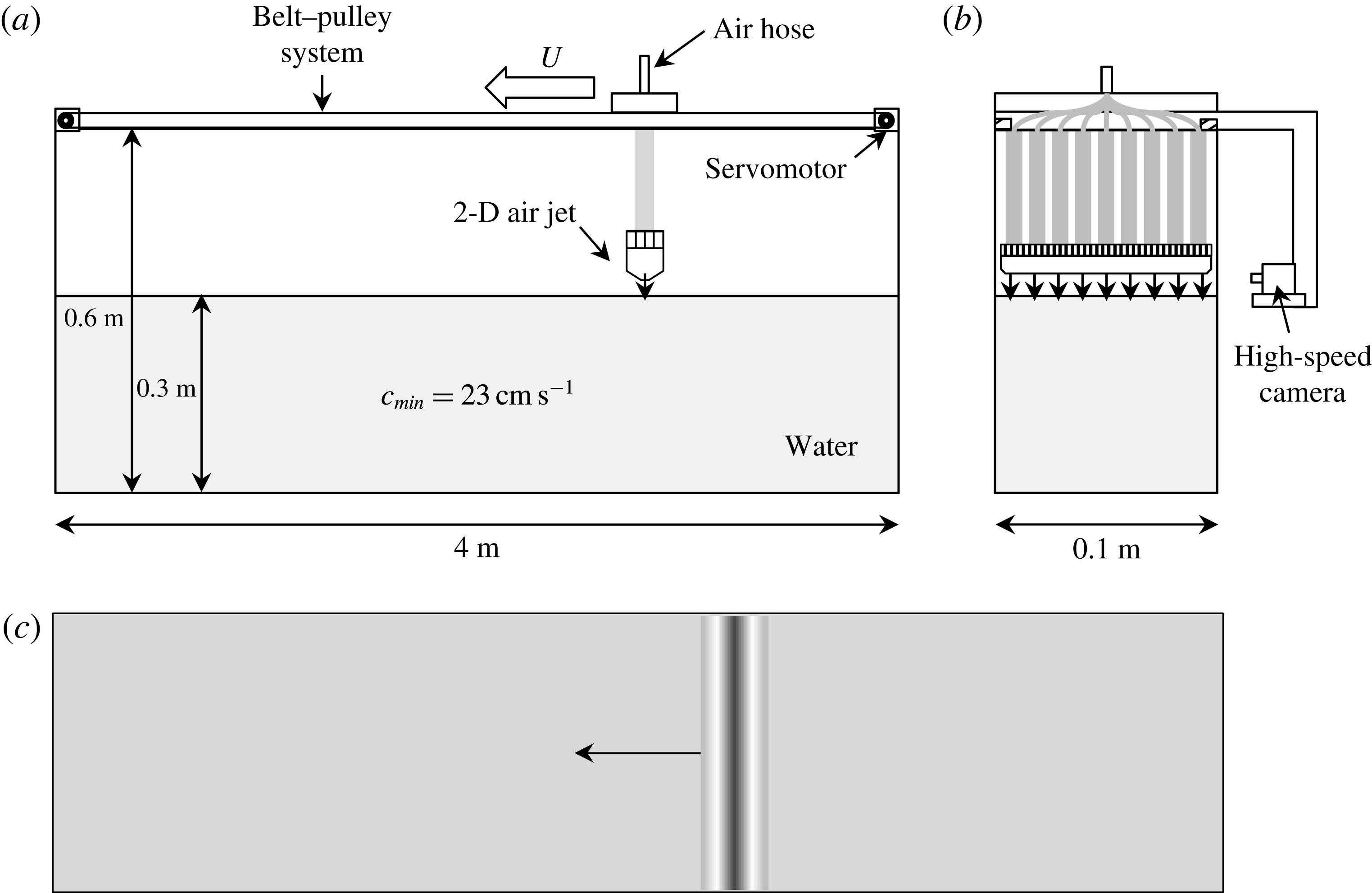
Figure 1. Experimental set-up. (a) Side view, (b) front view and (c) top view.
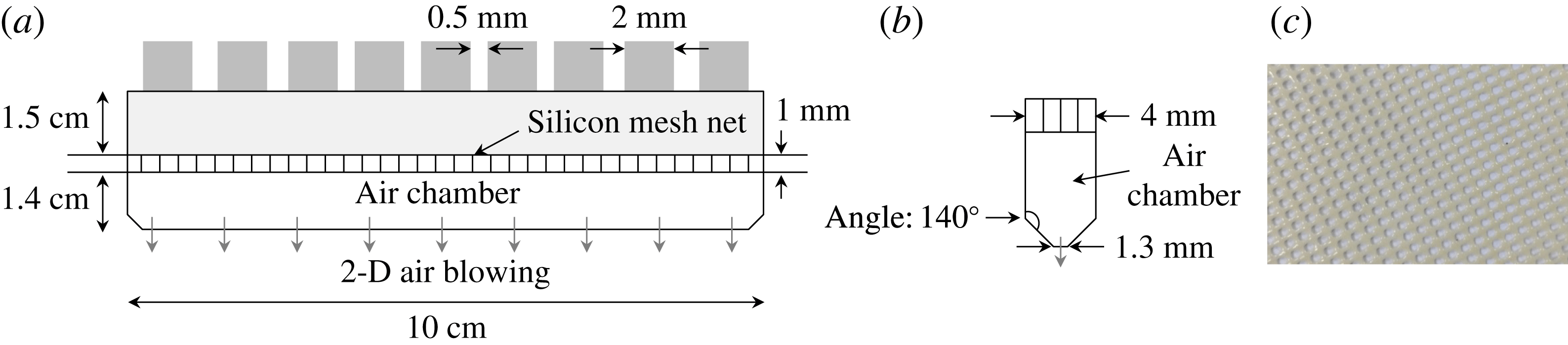
Figure 2. The main parts of the 2-D forcing mechanism: nine pipes, a silicon mesh net and a converging chamber with a narrow-slit exit. (a) Front view, (b) side view and (c) silicon mesh net (circular-pore number density of
 $13~\text{cm}^{-2}$
, pore diameter of 2 mm, thickness of 1 mm).
$13~\text{cm}^{-2}$
, pore diameter of 2 mm, thickness of 1 mm).

Figure 3. Slopes of 2-D depressions, i.e. dimensionless parameter
 $\unicode[STIX]{x1D716}=D/W$
, where
$\unicode[STIX]{x1D716}=D/W$
, where
 $D$
is the depth of the depression and
$D$
is the depth of the depression and
 $W$
is the width of the depression, when the air-blowing forcing is stationary, for (a)
$W$
is the width of the depression, when the air-blowing forcing is stationary, for (a)
 $\unicode[STIX]{x1D716}=0.04$
, (b)
$\unicode[STIX]{x1D716}=0.04$
, (b)
 $\unicode[STIX]{x1D716}=0.057$
, (c)
$\unicode[STIX]{x1D716}=0.057$
, (c)
 $\unicode[STIX]{x1D716}=0.08$
and (d)
$\unicode[STIX]{x1D716}=0.08$
and (d)
 $\unicode[STIX]{x1D716}=0.1$
.
$\unicode[STIX]{x1D716}=0.1$
.

Figure 4. Uniformity of the 2-D air-blowing forcing checked by the resultant steady-state wave profiles on the water surface at several transverse locations. (a–c) Side-view observations of steady-state wave profiles at three equally spaced positions in the transverse direction ((a)
 $1/4$
line, (b) centreline, (c)
$1/4$
line, (b) centreline, (c)
 $3/4$
line) for a forcing magnitude of
$3/4$
line) for a forcing magnitude of
 $\unicode[STIX]{x1D716}=0.08$
when the carriage is stationary (
$\unicode[STIX]{x1D716}=0.08$
when the carriage is stationary (
 $\unicode[STIX]{x1D6FC}=0$
). (d–f) Side-view observations of steady-state wave profiles at three equally spaced positions in the transverse direction ((d)
$\unicode[STIX]{x1D6FC}=0$
). (d–f) Side-view observations of steady-state wave profiles at three equally spaced positions in the transverse direction ((d)
 $1/4$
line, (e) centreline, (f)
$1/4$
line, (e) centreline, (f)
 $3/4$
line) for a forcing magnitude of
$3/4$
line) for a forcing magnitude of
 $\unicode[STIX]{x1D716}=0.08$
when the carriage is moving from right to left with a speed of
$\unicode[STIX]{x1D716}=0.08$
when the carriage is moving from right to left with a speed of
 $\unicode[STIX]{x1D6FC}=0.913$
.
$\unicode[STIX]{x1D6FC}=0.913$
.
In the preliminary test, the uniformity of the 2-D air-blowing forcing was checked by the resultant steady-state wave profiles on the water surface at several transverse locations. Figure 4(a–c) shows the observed wave profiles at three equally spaced positions in the transverse direction (
 $1/4$
line, centreline,
$1/4$
line, centreline,
 $3/4$
line) for a forcing magnitude of
$3/4$
line) for a forcing magnitude of
 $\unicode[STIX]{x1D716}=0.08$
when the carriage was stationary (
$\unicode[STIX]{x1D716}=0.08$
when the carriage was stationary (
 $\unicode[STIX]{x1D6FC}=0$
). The downward arrows in the figure denote the positions of the air-blowing forcings. As shown, small-amplitude depressions were observed below the stationary forcings and each depression was almost the same. Figure 4(d–f) shows the wave profiles at the same positions as those of figure 4(a–c) for a forcing magnitude of
$\unicode[STIX]{x1D6FC}=0$
). The downward arrows in the figure denote the positions of the air-blowing forcings. As shown, small-amplitude depressions were observed below the stationary forcings and each depression was almost the same. Figure 4(d–f) shows the wave profiles at the same positions as those of figure 4(a–c) for a forcing magnitude of
 $\unicode[STIX]{x1D716}=0.08$
when the carriage was moving from right to left with a speed of
$\unicode[STIX]{x1D716}=0.08$
when the carriage was moving from right to left with a speed of
 $\unicode[STIX]{x1D6FC}=0.913$
. In this exemplary non-stationary case, the resultant steady-state wave profiles were observed behind the moving forcing. These are actually 2-D gravity–capillary solitary waves which will be described in more detail in the next section. As shown, the three wave profiles were almost identical to one another.
$\unicode[STIX]{x1D6FC}=0.913$
. In this exemplary non-stationary case, the resultant steady-state wave profiles were observed behind the moving forcing. These are actually 2-D gravity–capillary solitary waves which will be described in more detail in the next section. As shown, the three wave profiles were almost identical to one another.
3 Generation of 2-D gravity–capillary solitary waves
Figure 5 shows side-view observations of steady-state surface-wave profiles according to the forcing speed (
 $\unicode[STIX]{x1D6FC}=0.87$
–1.1) when the forcing magnitude was fixed to be
$\unicode[STIX]{x1D6FC}=0.87$
–1.1) when the forcing magnitude was fixed to be
 $\unicode[STIX]{x1D716}=0.08$
. Like in figure 4, the downward arrow denotes the position of the moving forcing. At the lowest forcing speed
$\unicode[STIX]{x1D716}=0.08$
. Like in figure 4, the downward arrow denotes the position of the moving forcing. At the lowest forcing speed
 $\unicode[STIX]{x1D6FC}=0.87$
, a small-amplitude depression was observed just below the left-moving forcing (figure 5
a), which resembled the small-amplitude depression when the carriage was stationary (figure 4
a–c). Then, as the forcing speed was increased (
$\unicode[STIX]{x1D6FC}=0.87$
, a small-amplitude depression was observed just below the left-moving forcing (figure 5
a), which resembled the small-amplitude depression when the carriage was stationary (figure 4
a–c). Then, as the forcing speed was increased (
 $0.896<\unicode[STIX]{x1D6FC}<0.995$
), solitary-wave-like depressions were observed behind the left-moving forcing (figure 5
b–f). In this speed range, as the forcing speed
$0.896<\unicode[STIX]{x1D6FC}<0.995$
), solitary-wave-like depressions were observed behind the left-moving forcing (figure 5
b–f). In this speed range, as the forcing speed
 $\unicode[STIX]{x1D6FC}$
increased, the depths of these solitary-wave-like depressions decreased and their positions became farther away from the forcing. As the forcing speed further increased close to the minimum phase speed, for example
$\unicode[STIX]{x1D6FC}$
increased, the depths of these solitary-wave-like depressions decreased and their positions became farther away from the forcing. As the forcing speed further increased close to the minimum phase speed, for example
 $\unicode[STIX]{x1D6FC}=0.995$
, the steady surface-wave profile (figure 5
g) changed little compared with that of
$\unicode[STIX]{x1D6FC}=0.995$
, the steady surface-wave profile (figure 5
g) changed little compared with that of
 $\unicode[STIX]{x1D6FC}=0.97$
(figure 5
f). When the forcing speed was larger than the minimum phase speed, for example
$\unicode[STIX]{x1D6FC}=0.97$
(figure 5
f). When the forcing speed was larger than the minimum phase speed, for example
 $\unicode[STIX]{x1D6FC}=1.1$
, a pair of short and long linear waves was observed ahead of and behind the left-moving forcing, the wavelengths of which were 10 mm and 30 mm respectively (figure 5
h). Figures 6–9 show time histories of 2-D surface-wave profiles at different times at forcing speeds of
$\unicode[STIX]{x1D6FC}=1.1$
, a pair of short and long linear waves was observed ahead of and behind the left-moving forcing, the wavelengths of which were 10 mm and 30 mm respectively (figure 5
h). Figures 6–9 show time histories of 2-D surface-wave profiles at different times at forcing speeds of
 $\unicode[STIX]{x1D6FC}=0.87$
, 0.93, 0.995, 1.1 for the fixed forcing magnitude
$\unicode[STIX]{x1D6FC}=0.87$
, 0.93, 0.995, 1.1 for the fixed forcing magnitude
 $\unicode[STIX]{x1D716}=0.08$
, until steady states are reached. Compared with the just-mentioned steady surface-wave profiles, unsteady patterns of surface-wave profiles were also observed within a certain narrow forcing speed range near
$\unicode[STIX]{x1D716}=0.08$
, until steady states are reached. Compared with the just-mentioned steady surface-wave profiles, unsteady patterns of surface-wave profiles were also observed within a certain narrow forcing speed range near
 $\unicode[STIX]{x1D6FC}=1$
(
$\unicode[STIX]{x1D6FC}=1$
(
 $\unicode[STIX]{x1D6FC}=1$
–1.1). Figure 10(a–f) shows a series of temporal snapshots of surface-wave profiles for a forcing speed of
$\unicode[STIX]{x1D6FC}=1$
–1.1). Figure 10(a–f) shows a series of temporal snapshots of surface-wave profiles for a forcing speed of
 $\unicode[STIX]{x1D6FC}=1.02$
, with a time difference of 0.59 s between each snapshot. Figure 10(a,f) is the same, and thus periodic, and the period of this unsteady wave pattern is approximately 3 s. In the figures, what is repeated looks like continuous shedding of a local depression behind the left-moving forcing. For higher forcing speeds
$\unicode[STIX]{x1D6FC}=1.02$
, with a time difference of 0.59 s between each snapshot. Figure 10(a,f) is the same, and thus periodic, and the period of this unsteady wave pattern is approximately 3 s. In the figures, what is repeated looks like continuous shedding of a local depression behind the left-moving forcing. For higher forcing speeds
 $\unicode[STIX]{x1D6FC}<1.1$
, similar periodic surface-wave patterns are observed, but with shorter shedding periods.
$\unicode[STIX]{x1D6FC}<1.1$
, similar periodic surface-wave patterns are observed, but with shorter shedding periods.

Figure 5. Side-view observation of steady-state surface-wave profiles according to the forcing speed
 $\unicode[STIX]{x1D6FC}$
, for the fixed forcing magnitude
$\unicode[STIX]{x1D6FC}$
, for the fixed forcing magnitude
 $\unicode[STIX]{x1D716}=0.08$
, for (a)
$\unicode[STIX]{x1D716}=0.08$
, for (a)
 $\unicode[STIX]{x1D6FC}=0.87$
, (b)
$\unicode[STIX]{x1D6FC}=0.87$
, (b)
 $\unicode[STIX]{x1D6FC}=0.896$
, (c)
$\unicode[STIX]{x1D6FC}=0.896$
, (c)
 $\unicode[STIX]{x1D6FC}=0.913$
, (d)
$\unicode[STIX]{x1D6FC}=0.913$
, (d)
 $\unicode[STIX]{x1D6FC}=0.93$
, (e)
$\unicode[STIX]{x1D6FC}=0.93$
, (e)
 $\unicode[STIX]{x1D6FC}=0.956$
, (f)
$\unicode[STIX]{x1D6FC}=0.956$
, (f)
 $\unicode[STIX]{x1D6FC}=0.97$
, (g)
$\unicode[STIX]{x1D6FC}=0.97$
, (g)
 $\unicode[STIX]{x1D6FC}=0.995$
and (h)
$\unicode[STIX]{x1D6FC}=0.995$
and (h)
 $\unicode[STIX]{x1D6FC}=1.1$
.
$\unicode[STIX]{x1D6FC}=1.1$
.

Figure 6. Time history of side-view observation of 2-D surface-wave profiles at a forcing speed of
 $\unicode[STIX]{x1D6FC}=0.87$
, for the fixed forcing magnitude
$\unicode[STIX]{x1D6FC}=0.87$
, for the fixed forcing magnitude
 $\unicode[STIX]{x1D716}=0.08$
, until a steady state is reached.
$\unicode[STIX]{x1D716}=0.08$
, until a steady state is reached.

Figure 7. Time history of side-view observation of 2-D surface-wave profiles at a forcing speed of
 $\unicode[STIX]{x1D6FC}=0.93$
, for the fixed forcing magnitude
$\unicode[STIX]{x1D6FC}=0.93$
, for the fixed forcing magnitude
 $\unicode[STIX]{x1D716}=0.08$
, until a steady state is reached.
$\unicode[STIX]{x1D716}=0.08$
, until a steady state is reached.

Figure 8. Time history of side-view observation of 2-D surface-wave profiles at a forcing speed of
 $\unicode[STIX]{x1D6FC}=0.995$
, for the fixed forcing magnitude
$\unicode[STIX]{x1D6FC}=0.995$
, for the fixed forcing magnitude
 $\unicode[STIX]{x1D716}=0.08$
, until a steady state is reached.
$\unicode[STIX]{x1D716}=0.08$
, until a steady state is reached.

Figure 9. Time history of side-view observation of 2-D surface-wave profiles at a forcing speed of
 $\unicode[STIX]{x1D6FC}=1.1$
, for the fixed forcing magnitude
$\unicode[STIX]{x1D6FC}=1.1$
, for the fixed forcing magnitude
 $\unicode[STIX]{x1D716}=0.08$
, until a steady state is reached.
$\unicode[STIX]{x1D716}=0.08$
, until a steady state is reached.

Figure 10. Side-view observation of unsteady surface-wave profiles when the forcing speed is
 $\unicode[STIX]{x1D6FC}=1.02$
, for the fixed forcing magnitude
$\unicode[STIX]{x1D6FC}=1.02$
, for the fixed forcing magnitude
 $\unicode[STIX]{x1D716}=0.08$
. The time interval between each snapshot is 0.59 s.
$\unicode[STIX]{x1D716}=0.08$
. The time interval between each snapshot is 0.59 s.
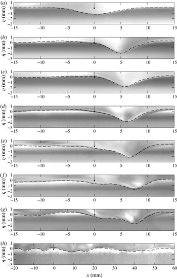
Figure 11. Comparison between the experimentally observed surface-wave profiles (figure 5) and the model-based (3.1) numerically obtained wave profiles (dashed curves) for the fixed forcing magnitude
 $\unicode[STIX]{x1D716}=0.08$
, for (a)
$\unicode[STIX]{x1D716}=0.08$
, for (a)
 $\unicode[STIX]{x1D6FC}=0.87$
, (b)
$\unicode[STIX]{x1D6FC}=0.87$
, (b)
 $\unicode[STIX]{x1D6FC}=0.896$
, (c)
$\unicode[STIX]{x1D6FC}=0.896$
, (c)
 $\unicode[STIX]{x1D6FC}=0.913$
, (d)
$\unicode[STIX]{x1D6FC}=0.913$
, (d)
 $\unicode[STIX]{x1D6FC}=0.93$
, (e)
$\unicode[STIX]{x1D6FC}=0.93$
, (e)
 $\unicode[STIX]{x1D6FC}=0.956$
, (f)
$\unicode[STIX]{x1D6FC}=0.956$
, (f)
 $\unicode[STIX]{x1D6FC}=0.97$
, (g)
$\unicode[STIX]{x1D6FC}=0.97$
, (g)
 $\unicode[STIX]{x1D6FC}=0.995$
and (h)
$\unicode[STIX]{x1D6FC}=0.995$
and (h)
 $\unicode[STIX]{x1D6FC}=1.1$
.
$\unicode[STIX]{x1D6FC}=1.1$
.
All of these experimentally observed wave profiles are compared with those from the following 2-D model equation which admits deep-water gravity–capillary solitary wave solutions near the minimum phase speed
 $c_{min}$
, in the presence of viscous damping and forcing (Cho et al.
Reference Cho, Diorio, Akylas and Duncan2011):
$c_{min}$
, in the presence of viscous damping and forcing (Cho et al.
Reference Cho, Diorio, Akylas and Duncan2011):
 $$\begin{eqnarray}\unicode[STIX]{x1D702}_{t}+(\unicode[STIX]{x1D6FC}-{\textstyle \frac{1}{2}})\unicode[STIX]{x1D702}_{x}-\unicode[STIX]{x1D6FD}(\unicode[STIX]{x1D702}^{2})_{x}-{\textstyle \frac{1}{4}}\mathscr{H}\left\{\unicode[STIX]{x1D702}_{xx}-\unicode[STIX]{x1D702}\right\}-\widetilde{\unicode[STIX]{x1D708}}\unicode[STIX]{x1D702}_{xx}=Ap_{x},\end{eqnarray}$$
where
 $\unicode[STIX]{x1D702}(x,y)$
is the dimensionless wave elevation,
$\unicode[STIX]{x1D702}(x,y)$
is the dimensionless wave elevation,
 $t$
is the dimensionless time,
$t$
is the dimensionless time,
 $x$
is the dimensionless streamwise coordinate in the left-moving reference frame with speed
$x$
is the dimensionless streamwise coordinate in the left-moving reference frame with speed
 $\unicode[STIX]{x1D6FC}$
, the nonlinear coefficient
$\unicode[STIX]{x1D6FC}$
, the nonlinear coefficient
 $\unicode[STIX]{x1D6FD}=\sqrt{11/2}/8$
, the operator
$\unicode[STIX]{x1D6FD}=\sqrt{11/2}/8$
, the operator
 $\mathscr{H}$
is the spatial Hilbert transform, such that
$\mathscr{H}$
is the spatial Hilbert transform, such that
 $\mathscr{H}\{f\}=\mathscr{F}^{-1}\{-\text{i}\text{sgn}(k)\mathscr{F}(f)\}$
, with
$\mathscr{H}\{f\}=\mathscr{F}^{-1}\{-\text{i}\text{sgn}(k)\mathscr{F}(f)\}$
, with
 $\mathscr{F}\{f\}=1/2\unicode[STIX]{x03C0}\int _{-\infty }^{\infty }f(x)\text{e}^{-\text{i}kx}\,\text{d}x$
(
$\mathscr{F}\{f\}=1/2\unicode[STIX]{x03C0}\int _{-\infty }^{\infty }f(x)\text{e}^{-\text{i}kx}\,\text{d}x$
(
 $k$
is the wavenumber),
$k$
is the wavenumber),
 $A$
is the forcing magnitude,
$A$
is the forcing magnitude,
 $p(x)$
is the forcing function and the subscript means partial differentiation. In addition, the dimensionless kinematic viscosity is
$p(x)$
is the forcing function and the subscript means partial differentiation. In addition, the dimensionless kinematic viscosity is
 $\widetilde{\unicode[STIX]{x1D708}}=C\unicode[STIX]{x1D708}(4g)^{1/4}(\unicode[STIX]{x1D70C}/\unicode[STIX]{x1D70E})^{3/4}$
, where
$\widetilde{\unicode[STIX]{x1D708}}=C\unicode[STIX]{x1D708}(4g)^{1/4}(\unicode[STIX]{x1D70C}/\unicode[STIX]{x1D70E})^{3/4}$
, where
 $\unicode[STIX]{x1D708}$
is the kinematic viscosity of water,
$\unicode[STIX]{x1D708}$
is the kinematic viscosity of water,
 $C$
is the tuning parameter (
$C$
is the tuning parameter (
 $C=1$
for linear sinusoidal waves,
$C=1$
for linear sinusoidal waves,
 $C>1$
for nonlinear solitary waves), g is the gravitational acceleration,
$C>1$
for nonlinear solitary waves), g is the gravitational acceleration,
 $\unicode[STIX]{x1D70C}$
is the water density and
$\unicode[STIX]{x1D70C}$
is the water density and
 $\unicode[STIX]{x1D70E}$
is the surface tension. The detailed derivation of (3.1) is shown in appendix A. In the present work, we choose
$\unicode[STIX]{x1D70E}$
is the surface tension. The detailed derivation of (3.1) is shown in appendix A. In the present work, we choose
 $C=2.4$
,
$C=2.4$
,
 $p(x)=\exp (-2x^{2})$
,
$p(x)=\exp (-2x^{2})$
,
 $A=0.048$
, by trial and error, to find the computational results that agree with the experimental results in terms of speed-dependent behaviour both qualitatively and quantitatively. The computational domain size is
$A=0.048$
, by trial and error, to find the computational results that agree with the experimental results in terms of speed-dependent behaviour both qualitatively and quantitatively. The computational domain size is
 $-94<x<94$
with a spatial resolution of
$-94<x<94$
with a spatial resolution of
 $\text{d}x=0.18$
. We adopt the spectral method for the spatial computation and the predictor–corrector scheme for the temporal computation. For dimensional results, the characteristic length
$\text{d}x=0.18$
. We adopt the spectral method for the spatial computation and the predictor–corrector scheme for the temporal computation. For dimensional results, the characteristic length
 $L=\left(\unicode[STIX]{x1D70E}/\unicode[STIX]{x1D70C}g\right)^{1/2}=2.73$
mm and the characteristic time
$L=\left(\unicode[STIX]{x1D70E}/\unicode[STIX]{x1D70C}g\right)^{1/2}=2.73$
mm and the characteristic time
 $T=L/c_{min}=0.0118~\text{s}$
are used. Figures 11–16 show the model-based numerical results which are overlaid on the observed surface-wave profiles (figures 5–10) from the experiment. As shown, they agree with each other very well. In addition, to check that the solitary-wave-like depressions observed behind the left-moving forcing (figures 5
b–g or 11
b–g) are indeed solitary waves, we solve the following inviscid forcing-free steady model equation which adopts a solitary wave solution with a propagation speed
$T=L/c_{min}=0.0118~\text{s}$
are used. Figures 11–16 show the model-based numerical results which are overlaid on the observed surface-wave profiles (figures 5–10) from the experiment. As shown, they agree with each other very well. In addition, to check that the solitary-wave-like depressions observed behind the left-moving forcing (figures 5
b–g or 11
b–g) are indeed solitary waves, we solve the following inviscid forcing-free steady model equation which adopts a solitary wave solution with a propagation speed
 $\unicode[STIX]{x1D6FC}$
:
$\unicode[STIX]{x1D6FC}$
:
 $$\begin{eqnarray}(\unicode[STIX]{x1D6FC}-{\textstyle \frac{1}{2}})\unicode[STIX]{x1D702}_{x}-\unicode[STIX]{x1D6FD}(\unicode[STIX]{x1D702}^{2})_{x}-{\textstyle \frac{1}{4}}\mathscr{H}\left\{\unicode[STIX]{x1D702}_{xx}-\unicode[STIX]{x1D702}\right\}=0.\end{eqnarray}$$
Equation (3.2) is solved by a modified Petviashvili method (Cho Reference Cho2015) or the pseudo-arclength continuation method (Cho Reference Cho2014). In figure 17, for forcing speeds in the range
 $0.896<\unicode[STIX]{x1D6FC}<0.995$
, the computed forcing-free inviscid solitary wave solutions are compared with the solitary-wave-like depressions behind the left-moving forcing in figure 5(b–g). As shown in figure 17(a–e), for moving speeds in the range
$0.896<\unicode[STIX]{x1D6FC}<0.995$
, the computed forcing-free inviscid solitary wave solutions are compared with the solitary-wave-like depressions behind the left-moving forcing in figure 5(b–g). As shown in figure 17(a–e), for moving speeds in the range
 $0.896<\unicode[STIX]{x1D6FC}<0.97$
, they agree with each other very well, and, therefore, they are indeed 2-D gravity–capillary solitary waves. However, for the case
$0.896<\unicode[STIX]{x1D6FC}<0.97$
, they agree with each other very well, and, therefore, they are indeed 2-D gravity–capillary solitary waves. However, for the case
 $\unicode[STIX]{x1D6FC}=0.995$
, the depression in figure 17(f) does not agree with the solitary wave solution with a propagation speed of
$\unicode[STIX]{x1D6FC}=0.995$
, the depression in figure 17(f) does not agree with the solitary wave solution with a propagation speed of
 $\unicode[STIX]{x1D6FC}=0.995$
, and, therefore, the depression is not a solitary wave. The results are summarized in figure 18, which shows the relationship between the forcing speed
$\unicode[STIX]{x1D6FC}=0.995$
, and, therefore, the depression is not a solitary wave. The results are summarized in figure 18, which shows the relationship between the forcing speed
 $\unicode[STIX]{x1D6FC}$
and the maximum surface depression
$\unicode[STIX]{x1D6FC}$
and the maximum surface depression
 $h_{max}$
, depending on the forcing magnitude. For a fixed magnitude of forcing, there exists a critical speed
$h_{max}$
, depending on the forcing magnitude. For a fixed magnitude of forcing, there exists a critical speed
 $\unicode[STIX]{x1D6FC}_{crit}$
just after which nonlinear solitary waves are observed behind the moving forcing. As the speed below
$\unicode[STIX]{x1D6FC}_{crit}$
just after which nonlinear solitary waves are observed behind the moving forcing. As the speed below
 $\unicode[STIX]{x1D6FC}_{crit}$
increases, the depth of the simple depressions below the forcing increases. As the speed above
$\unicode[STIX]{x1D6FC}_{crit}$
increases, the depth of the simple depressions below the forcing increases. As the speed above
 $\unicode[STIX]{x1D6FC}_{crit}$
increases, the depth of depression of the solitary wave decreases. In addition, regardless of the forcing magnitude, the same solitary waves are observed if the forcing speeds are the same; that is, in the
$\unicode[STIX]{x1D6FC}_{crit}$
increases, the depth of depression of the solitary wave decreases. In addition, regardless of the forcing magnitude, the same solitary waves are observed if the forcing speeds are the same; that is, in the
 $\unicode[STIX]{x1D6FC}$
–
$\unicode[STIX]{x1D6FC}$
–
 $h_{max}$
diagram (figure 18), they fall on the same negative-slope curve as is predicted by the model equation (3.2) for the free inviscid solitary waves.
$h_{max}$
diagram (figure 18), they fall on the same negative-slope curve as is predicted by the model equation (3.2) for the free inviscid solitary waves.

Figure 12. Time history: comparison between the experimentally observed surface-wave profiles (figure 6) and the model-based (3.1) numerically obtained wave profiles (dashed curves) at a forcing speed of
 $\unicode[STIX]{x1D6FC}=0.87$
, for the fixed forcing magnitude
$\unicode[STIX]{x1D6FC}=0.87$
, for the fixed forcing magnitude
 $\unicode[STIX]{x1D716}=0.08$
, until a steady state is reached.
$\unicode[STIX]{x1D716}=0.08$
, until a steady state is reached.

Figure 13. Time history: comparison between the experimentally observed surface-wave profiles (figure 7) and the model-based (3.1) numerically obtained wave profiles (dashed curves) at a forcing speed of
 $\unicode[STIX]{x1D6FC}=0.93$
, for the fixed forcing magnitude
$\unicode[STIX]{x1D6FC}=0.93$
, for the fixed forcing magnitude
 $\unicode[STIX]{x1D716}=0.08$
, until a steady state is reached.
$\unicode[STIX]{x1D716}=0.08$
, until a steady state is reached.

Figure 14. Time history: comparison between the experimentally observed surface-wave profiles (figure 8) and the model-based (3.1) numerically obtained wave profiles (dashed curves) at a forcing speed of
 $\unicode[STIX]{x1D6FC}=0.995$
, for the fixed forcing magnitude
$\unicode[STIX]{x1D6FC}=0.995$
, for the fixed forcing magnitude
 $\unicode[STIX]{x1D716}=0.08$
, until a steady state is reached.
$\unicode[STIX]{x1D716}=0.08$
, until a steady state is reached.

Figure 15. Time history: comparison between the experimentally observed surface-wave profiles (figure 9) and the model-based (3.1) numerically obtained wave profiles (dashed curves) at a forcing speed of
 $\unicode[STIX]{x1D6FC}=1.1$
, for the fixed forcing magnitude
$\unicode[STIX]{x1D6FC}=1.1$
, for the fixed forcing magnitude
 $\unicode[STIX]{x1D716}=0.08$
, until a steady state is reached.
$\unicode[STIX]{x1D716}=0.08$
, until a steady state is reached.

Figure 16. Comparison between the experimentally observed surface-wave profiles (figure 10) and the model-based (3.1) computationally obtained wave profiles (dashed curves) when the forcing speed
 $\unicode[STIX]{x1D6FC}=1.02$
for the fixed forcing magnitude
$\unicode[STIX]{x1D6FC}=1.02$
for the fixed forcing magnitude
 $\unicode[STIX]{x1D716}=0.08$
. The time interval between each snapshot is 0.59 s.
$\unicode[STIX]{x1D716}=0.08$
. The time interval between each snapshot is 0.59 s.

Figure 17. Comparison among the experimentally observed solitary-wave-like depressions behind the left-moving forcing (figure 5
b–g), the model-based (3.1) forced viscous wave profiles (dashed curves, figure 11
b–g) and the model-based (3.2) forcing-free inviscid solitary wave profiles (solid curves), for (a)
 $\unicode[STIX]{x1D6FC}=0.896$
, (b)
$\unicode[STIX]{x1D6FC}=0.896$
, (b)
 $\unicode[STIX]{x1D6FC}=0.913$
, (c)
$\unicode[STIX]{x1D6FC}=0.913$
, (c)
 $\unicode[STIX]{x1D6FC}=0.93$
, (d)
$\unicode[STIX]{x1D6FC}=0.93$
, (d)
 $\unicode[STIX]{x1D6FC}=0.956$
, (e)
$\unicode[STIX]{x1D6FC}=0.956$
, (e)
 $\unicode[STIX]{x1D6FC}=0.97$
and (f)
$\unicode[STIX]{x1D6FC}=0.97$
and (f)
 $\unicode[STIX]{x1D6FC}=0.995$
.
$\unicode[STIX]{x1D6FC}=0.995$
.
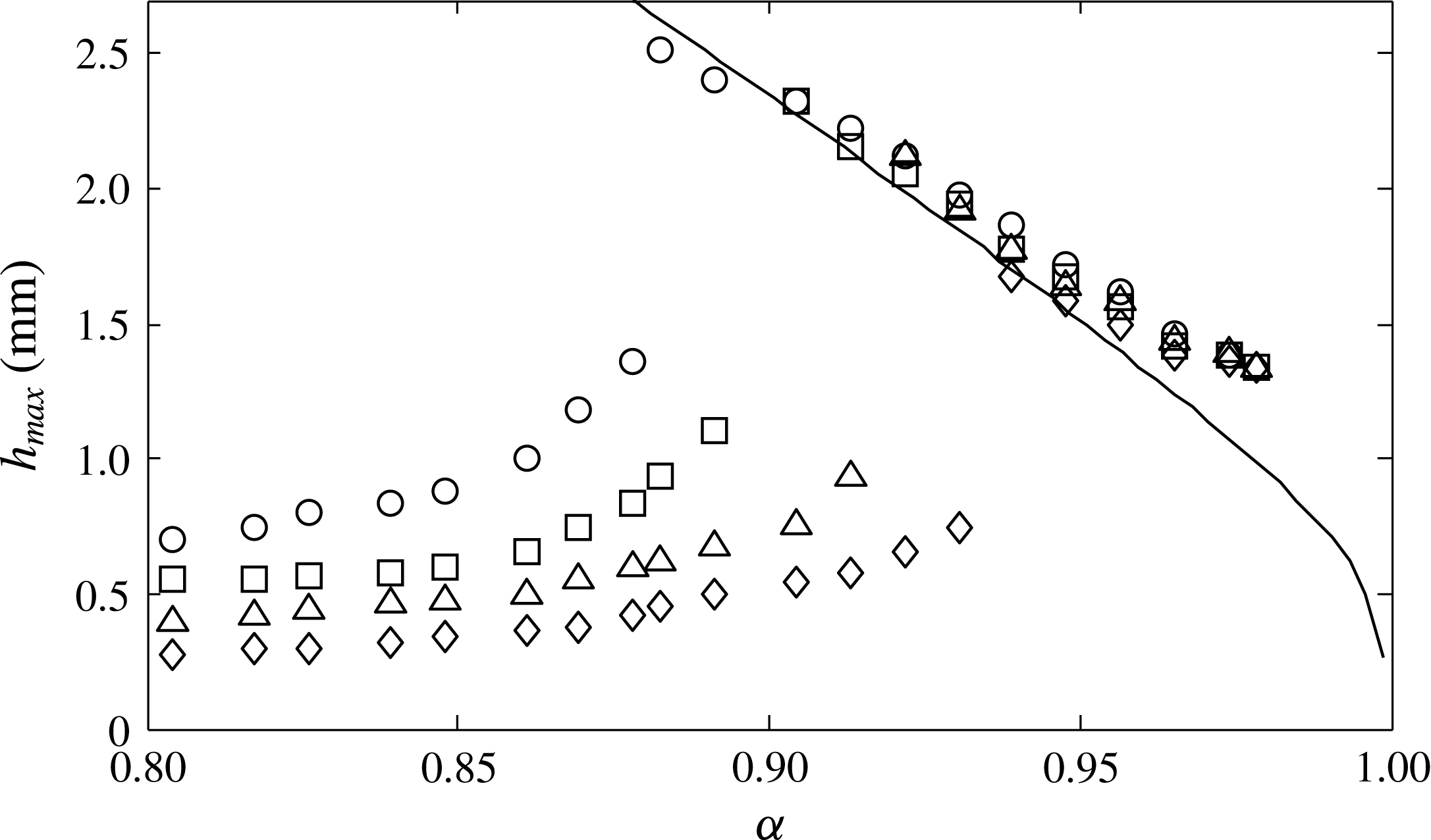
Figure 18. Maximum surface depression
 $h_{max}$
of the observed 2-D waves according to the forcing speed
$h_{max}$
of the observed 2-D waves according to the forcing speed
 $\unicode[STIX]{x1D6FC}$
for different magnitudes of the 2-D air-blowing forcing:
$\unicode[STIX]{x1D6FC}$
for different magnitudes of the 2-D air-blowing forcing:
 $\unicode[STIX]{x1D716}=0.04$
(♢),
$\unicode[STIX]{x1D716}=0.04$
(♢),
 $\unicode[STIX]{x1D716}=0.057$
(▵),
$\unicode[STIX]{x1D716}=0.057$
(▵),
 $\unicode[STIX]{x1D716}=0.08$
(▫),
$\unicode[STIX]{x1D716}=0.08$
(▫),
 $\unicode[STIX]{x1D716}=0.1$
(○). The negative-slope solid curve is predicted by the model (3.2) for inviscid solitary waves.
$\unicode[STIX]{x1D716}=0.1$
(○). The negative-slope solid curve is predicted by the model (3.2) for inviscid solitary waves.
4 Decaying behaviour of 2-D gravity–capillary solitary waves

Figure 19. Slanted 3-D view of the decaying behaviour of an initial 2-D gravity–capillary solitary wave for
 $\unicode[STIX]{x1D6FC}=0.93$
at
$\unicode[STIX]{x1D6FC}=0.93$
at
 $t=0.35$
s, 0.47 s, 0.59 s and 0.71 s after turning off the forcing. (a–d) Experiment. (e–h) Computation (4.1). All of the results are taken from the fixed reference frame.
$t=0.35$
s, 0.47 s, 0.59 s and 0.71 s after turning off the forcing. (a–d) Experiment. (e–h) Computation (4.1). All of the results are taken from the fixed reference frame.

Figure 20. Side view of the decaying behaviour of an initial 2-D gravity–capillary solitary wave for
 $\unicode[STIX]{x1D6FC}=0.93$
at
$\unicode[STIX]{x1D6FC}=0.93$
at
 $t=0.35$
s, 0.47 s, 0.59 s and 0.71 s after turning off the forcing. (a–d) Experiment. (e–h) Computation (equation (4.1), dashed curves). All of the results are taken from the fixed reference frame.
$t=0.35$
s, 0.47 s, 0.59 s and 0.71 s after turning off the forcing. (a–d) Experiment. (e–h) Computation (equation (4.1), dashed curves). All of the results are taken from the fixed reference frame.

Figure 21. Rear view of the decaying behaviour of an initial 2-D gravity–capillary solitary wave for
 $\unicode[STIX]{x1D6FC}=0.93$
at
$\unicode[STIX]{x1D6FC}=0.93$
at
 $t=0.35$
s, 0.47 s, 0.59 s and 0.71 s after turning off the forcing. (a–d) Experiment. (e–h) Computation (equation (4.1), dashed curves). All of the results are taken from the fixed reference frame.
$t=0.35$
s, 0.47 s, 0.59 s and 0.71 s after turning off the forcing. (a–d) Experiment. (e–h) Computation (equation (4.1), dashed curves). All of the results are taken from the fixed reference frame.
In the previous section, we observed that 2-D gravity–capillary solitary waves are generated behind the moving forcing (
 $\unicode[STIX]{x1D716}=0.08$
) for the speed range
$\unicode[STIX]{x1D716}=0.08$
) for the speed range
 $0.896<\unicode[STIX]{x1D6FC}<0.97$
. To see the decaying behaviour of free gravity–capillary solitary waves, for example for the speed
$0.896<\unicode[STIX]{x1D6FC}<0.97$
. To see the decaying behaviour of free gravity–capillary solitary waves, for example for the speed
 $\unicode[STIX]{x1D6FC}=0.93$
, we turned off the airflow after the steady-state solitary wave was formed behind the forcing. Then, the solitary wave disappeared almost instantly. Figures 19(a–d), 20(a–d) and 21(a–d) show the observed decaying behaviour of the initial forced 2-D gravity–capillary solitary wave for
$\unicode[STIX]{x1D6FC}=0.93$
, we turned off the airflow after the steady-state solitary wave was formed behind the forcing. Then, the solitary wave disappeared almost instantly. Figures 19(a–d), 20(a–d) and 21(a–d) show the observed decaying behaviour of the initial forced 2-D gravity–capillary solitary wave for
 $\unicode[STIX]{x1D6FC}=0.93$
at
$\unicode[STIX]{x1D6FC}=0.93$
at
 $t=0.35$
s, 0.47 s, 0.59 s and 0.71 s after the forcing was turned off, in 3-D slanted view, side view and rear view respectively. These images were taken from fixed cameras on the laboratory floor. Also shown are the corresponding computational results (figure 19
e–h, dashed curves in figures 20
e–h, 21
e–h), which are expressed in the fixed reference frame at
$t=0.35$
s, 0.47 s, 0.59 s and 0.71 s after the forcing was turned off, in 3-D slanted view, side view and rear view respectively. These images were taken from fixed cameras on the laboratory floor. Also shown are the corresponding computational results (figure 19
e–h, dashed curves in figures 20
e–h, 21
e–h), which are expressed in the fixed reference frame at
 $t=0.35$
s, 0.47 s, 0.59 s and 0.71 s. These are obtained by solving the following forcing-free viscous 3-D model equation with
$t=0.35$
s, 0.47 s, 0.59 s and 0.71 s. These are obtained by solving the following forcing-free viscous 3-D model equation with
 $C=2.4$
extended from the 2-D model equation (3.1) (Cho et al.
Reference Cho, Diorio, Akylas and Duncan2011):
$C=2.4$
extended from the 2-D model equation (3.1) (Cho et al.
Reference Cho, Diorio, Akylas and Duncan2011):
 $$\begin{eqnarray}\unicode[STIX]{x1D702}_{t}+(\unicode[STIX]{x1D6FC}-{\textstyle \frac{1}{2}})\unicode[STIX]{x1D702}_{x}-\unicode[STIX]{x1D6FD}(\unicode[STIX]{x1D702}^{2})_{x}-{\textstyle \frac{1}{4}}\mathscr{H}\left\{\unicode[STIX]{x1D702}_{xx}+2\unicode[STIX]{x1D702}_{yy}-\unicode[STIX]{x1D702}\right\}-\widetilde{\unicode[STIX]{x1D708}}(\unicode[STIX]{x1D702}_{xx}+\unicode[STIX]{x1D702}_{yy})=0.\end{eqnarray}$$
The initial condition in solving the above equation is the 2-D surface-wave profile for
 $\unicode[STIX]{x1D6FC}=0.93$
obtained from the forced model equation (3.1) with
$\unicode[STIX]{x1D6FC}=0.93$
obtained from the forced model equation (3.1) with
 $C=2.4$
. As shown in figures 19–21, the experimental results and computational results (dashed curves) agree with each other very well.
$C=2.4$
. As shown in figures 19–21, the experimental results and computational results (dashed curves) agree with each other very well.
5 Transverse instability of 2-D gravity–capillary solitary waves

Figure 22. Three-dimensional slanted view of the observed behaviour of an initial 2-D gravity–capillary solitary wave for
 $\unicode[STIX]{x1D6FC}=0.93$
at
$\unicode[STIX]{x1D6FC}=0.93$
at
 $t=0.35$
s, 0.47 s, 0.59 s and 0.71 s, after the forcing motion is stopped and, very shortly afterwards, the airflow is turned off. (a–d) Experiment. (e–h) Computation (4.1) and (5.1). All of the results are taken from the fixed reference frame.
$t=0.35$
s, 0.47 s, 0.59 s and 0.71 s, after the forcing motion is stopped and, very shortly afterwards, the airflow is turned off. (a–d) Experiment. (e–h) Computation (4.1) and (5.1). All of the results are taken from the fixed reference frame.

Figure 23. Centreline side view of the observed behaviour of an initial 2-D gravity–capillary solitary wave for
 $\unicode[STIX]{x1D6FC}=0.93$
at
$\unicode[STIX]{x1D6FC}=0.93$
at
 $t=0.35$
s, 0.47 s, 0.59 s and 0.71 s, after the forcing motion is stopped and, very shortly afterwards, the airflow is turned off. (a–d) Experiment. (e–h) Computation (4.1) and (5.1). In (e–h), centreline side-view profiles of forcing-free 3-D inviscid solitary waves ((5.2), solid curves) with propagation speeds of
$t=0.35$
s, 0.47 s, 0.59 s and 0.71 s, after the forcing motion is stopped and, very shortly afterwards, the airflow is turned off. (a–d) Experiment. (e–h) Computation (4.1) and (5.1). In (e–h), centreline side-view profiles of forcing-free 3-D inviscid solitary waves ((5.2), solid curves) with propagation speeds of
 $\unicode[STIX]{x1D6FC}=0.977$
, 0.968, 0.968 and 0.974 are overlaid. All of the results are taken from the fixed reference frame.
$\unicode[STIX]{x1D6FC}=0.977$
, 0.968, 0.968 and 0.974 are overlaid. All of the results are taken from the fixed reference frame.

Figure 24. Centreline rear view of the observed behaviour of an initial 2-D gravity–capillary solitary wave for
 $\unicode[STIX]{x1D6FC}=0.93$
at
$\unicode[STIX]{x1D6FC}=0.93$
at
 $t=0.35$
s, 0.47 s, 0.59 s and 0.71 s, after the forcing motion is stopped and, very shortly afterwards, the airflow is turned off. (a–d) Experiment. (e–h) Computation (4.1) and (5.1). In (e–h), centreline rear-view profiles of forcing-free 3-D inviscid solitary waves ((5.2), solid curves) with propagation speeds of
$t=0.35$
s, 0.47 s, 0.59 s and 0.71 s, after the forcing motion is stopped and, very shortly afterwards, the airflow is turned off. (a–d) Experiment. (e–h) Computation (4.1) and (5.1). In (e–h), centreline rear-view profiles of forcing-free 3-D inviscid solitary waves ((5.2), solid curves) with propagation speeds of
 $\unicode[STIX]{x1D6FC}=0.977$
, 0.968, 0.968 and 0.974 are overlaid. All of the results are taken from the fixed reference frame.
$\unicode[STIX]{x1D6FC}=0.977$
, 0.968, 0.968 and 0.974 are overlaid. All of the results are taken from the fixed reference frame.
In the previous section, we turned off the airflow (
 $\unicode[STIX]{x1D716}=0.08$
) when the 2-D steady-state solitary wave had already formed behind the moving forcing with a speed of
$\unicode[STIX]{x1D716}=0.08$
) when the 2-D steady-state solitary wave had already formed behind the moving forcing with a speed of
 $\unicode[STIX]{x1D6FC}=0.93$
. Then, in a very short time, the solitary wave shows a decaying behaviour with no variation in the transverse direction. Comparatively, in the present section, instead of turning off the airflow, we stop the translational motion of the forcing when the 2-D steady-state solitary wave has already formed behind the moving forcing with a speed of
$\unicode[STIX]{x1D6FC}=0.93$
. Then, in a very short time, the solitary wave shows a decaying behaviour with no variation in the transverse direction. Comparatively, in the present section, instead of turning off the airflow, we stop the translational motion of the forcing when the 2-D steady-state solitary wave has already formed behind the moving forcing with a speed of
 $\unicode[STIX]{x1D6FC}=0.93$
. Then, shortly afterwards, we turn off the airflow. As a result of this successive operation, we can observe the transverse instability of a forcing-free solitary wave. In the present experiment, the cause of the transverse instability is the existence of sidewalls. Figure 22(a–d) shows a 3-D slanted view of the observed behaviour of the initial 2-D gravity–capillary solitary wave for
$\unicode[STIX]{x1D6FC}=0.93$
. Then, shortly afterwards, we turn off the airflow. As a result of this successive operation, we can observe the transverse instability of a forcing-free solitary wave. In the present experiment, the cause of the transverse instability is the existence of sidewalls. Figure 22(a–d) shows a 3-D slanted view of the observed behaviour of the initial 2-D gravity–capillary solitary wave for
 $\unicode[STIX]{x1D6FC}=0.93$
at
$\unicode[STIX]{x1D6FC}=0.93$
at
 $t=0.35$
s, 0.47 s, 0.59 s and 0.71 s, after the forcing motion was stopped and, very shortly afterwards, the airflow was turned off. These images were taken from fixed cameras on the laboratory floor. In figure 22(a) (
$t=0.35$
s, 0.47 s, 0.59 s and 0.71 s, after the forcing motion was stopped and, very shortly afterwards, the airflow was turned off. These images were taken from fixed cameras on the laboratory floor. In figure 22(a) (
 $t=0.35$
s), near the centreline, one can see the starting formation of a 3-D solitary-wave-like depression. Between near the centreline and the walls, the surface profiles are 2-D depressions which are remnants from the initial 2-D gravity–capillary solitary wave. Then, in figure 22(b–d) (
$t=0.35$
s), near the centreline, one can see the starting formation of a 3-D solitary-wave-like depression. Between near the centreline and the walls, the surface profiles are 2-D depressions which are remnants from the initial 2-D gravity–capillary solitary wave. Then, in figure 22(b–d) (
 $t=0.47$
s, 0.59 s, 0.71 s), the 3-D solitary-wave-like depression near the centreline becomes more prominent and propagates stably to the left while the remaining 2-D depressions disappear due to viscous dissipation. Corresponding to figure 22(a–d) (3-D slanted view), figures 23(a–d) and 24(a–d) show the side view at the centreline and the rear view of the observed behaviour at the same instants. Also shown are corresponding computational results (figure 22
e–h, dashed curves in figures 23
e–h, 24
e–h), which are expressed in the fixed reference frame at
$t=0.47$
s, 0.59 s, 0.71 s), the 3-D solitary-wave-like depression near the centreline becomes more prominent and propagates stably to the left while the remaining 2-D depressions disappear due to viscous dissipation. Corresponding to figure 22(a–d) (3-D slanted view), figures 23(a–d) and 24(a–d) show the side view at the centreline and the rear view of the observed behaviour at the same instants. Also shown are corresponding computational results (figure 22
e–h, dashed curves in figures 23
e–h, 24
e–h), which are expressed in the fixed reference frame at
 $t=0.35$
s, 0.47 s, 0.59 s and 0.71 s. These are obtained by solving (4.1) with
$t=0.35$
s, 0.47 s, 0.59 s and 0.71 s. These are obtained by solving (4.1) with
 $C=2.4$
. The initial condition is the transversely perturbed 2-D surface-wave profile
$C=2.4$
. The initial condition is the transversely perturbed 2-D surface-wave profile
 $\widetilde{\unicode[STIX]{x1D702}}(x)$
for
$\widetilde{\unicode[STIX]{x1D702}}(x)$
for
 $\unicode[STIX]{x1D6FC}=0.93$
obtained from the forced model equation (3.1) with
$\unicode[STIX]{x1D6FC}=0.93$
obtained from the forced model equation (3.1) with
 $C=2.4$
,
$C=2.4$
,
 $$\begin{eqnarray}\unicode[STIX]{x1D702}(x,y,t=0)=\widetilde{\unicode[STIX]{x1D702}}(x)(1+\unicode[STIX]{x1D6FF}\cos (y/y_{lim})),\end{eqnarray}$$
where the dimensionless computational domain size in the
 $y$
direction is
$y$
direction is
 $-\unicode[STIX]{x03C0}y_{lim}<y<\unicode[STIX]{x03C0}y_{lim}$
. From the experiments, we see that the perturbations from sidewalls are symmetric. Thus, in the computation, we take the perturbation to be symmetric and, further, the fundamental-mode cosine function. Considering that the physical domain size in the transverse
$-\unicode[STIX]{x03C0}y_{lim}<y<\unicode[STIX]{x03C0}y_{lim}$
. From the experiments, we see that the perturbations from sidewalls are symmetric. Thus, in the computation, we take the perturbation to be symmetric and, further, the fundamental-mode cosine function. Considering that the physical domain size in the transverse
 $y$
direction is 100 mm, we take
$y$
direction is 100 mm, we take
 $y_{lim}=6$
, such that
$y_{lim}=6$
, such that
 $2\unicode[STIX]{x03C0}y_{lim}L=100$
mm, where
$2\unicode[STIX]{x03C0}y_{lim}L=100$
mm, where
 $L=2.73$
mm. The amount of the transverse perturbation
$L=2.73$
mm. The amount of the transverse perturbation
 $\unicode[STIX]{x1D6FF}$
is taken to be 0.15 (15 %), by trial and error, for a good agreement between experiments and computations. As shown in figures 22–24, the experimental results and computational results (dashed curves) agree with each other very well. In particular, in figures 23(e–h) and 24(e–h) respectively, side-view centreline and rear-view profiles of forcing-free inviscid 3-D solitary waves with certain propagation speeds (solid curves) are overlaid on the dashed surface depressions. The forcing-free inviscid 3-D solitary waves are obtained from the following model equation (Cho et al.
Reference Cho, Diorio, Akylas and Duncan2011) using the modified Petviashvili method (Cho Reference Cho2015) or the pseudo-arclength continuation method (Cho Reference Cho2014):
$\unicode[STIX]{x1D6FF}$
is taken to be 0.15 (15 %), by trial and error, for a good agreement between experiments and computations. As shown in figures 22–24, the experimental results and computational results (dashed curves) agree with each other very well. In particular, in figures 23(e–h) and 24(e–h) respectively, side-view centreline and rear-view profiles of forcing-free inviscid 3-D solitary waves with certain propagation speeds (solid curves) are overlaid on the dashed surface depressions. The forcing-free inviscid 3-D solitary waves are obtained from the following model equation (Cho et al.
Reference Cho, Diorio, Akylas and Duncan2011) using the modified Petviashvili method (Cho Reference Cho2015) or the pseudo-arclength continuation method (Cho Reference Cho2014):
 $$\begin{eqnarray}(\unicode[STIX]{x1D6FC}-{\textstyle \frac{1}{2}})\unicode[STIX]{x1D702}_{x}-\unicode[STIX]{x1D6FD}(\unicode[STIX]{x1D702}^{2})_{x}-{\textstyle \frac{1}{4}}\mathscr{H}\left\{\unicode[STIX]{x1D702}_{xx}+2\unicode[STIX]{x1D702}_{yy}-\unicode[STIX]{x1D702}\right\}=0.\end{eqnarray}$$
We see that, at each instant
 $t=0.35$
s, 0.47 s, 0.59 s, 0.71 s, the 3-D solitary-wave-like depressions are indeed forcing-free inviscid 3-D gravity–capillary solitary waves propagating with speeds of
$t=0.35$
s, 0.47 s, 0.59 s, 0.71 s, the 3-D solitary-wave-like depressions are indeed forcing-free inviscid 3-D gravity–capillary solitary waves propagating with speeds of
 $\unicode[STIX]{x1D6FC}=0.977$
, 0.968, 0.968 and 0.974 respectively under the influence of viscosity. Here, in the 3-D forcing-free viscous computation, we take
$\unicode[STIX]{x1D6FC}=0.977$
, 0.968, 0.968 and 0.974 respectively under the influence of viscosity. Here, in the 3-D forcing-free viscous computation, we take
 $C=2.4$
, by trial and error, for a good agreement between experiments and computations.
$C=2.4$
, by trial and error, for a good agreement between experiments and computations.
6 Theoretical proof of the transverse instability of 2-D gravity–capillary solitary waves
In § 5, the transverse instability of 2-D gravity–capillary solitary waves on deep water was observed in an experiment and was confirmed numerically using a theoretical model equation that admits gravity–capillary solitary wave solutions near
 $c_{min}$
. In the present section, based on a linear stability analysis using the same model equation without viscosity, we will give a theoretical proof of the transverse instability of the 2-D gravity–capillary solitary waves on deep water (
$c_{min}$
. In the present section, based on a linear stability analysis using the same model equation without viscosity, we will give a theoretical proof of the transverse instability of the 2-D gravity–capillary solitary waves on deep water (
 $\unicode[STIX]{x2202}E/\unicode[STIX]{x2202}\unicode[STIX]{x1D6FC}<0$
), where
$\unicode[STIX]{x2202}E/\unicode[STIX]{x2202}\unicode[STIX]{x1D6FC}<0$
), where
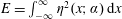 $E=\int _{-\infty }^{\infty }\unicode[STIX]{x1D702}^{2}(x;\unicode[STIX]{x1D6FC})\,\text{d}x$
is the energy of the solitary wave. First, let us consider a solution
$E=\int _{-\infty }^{\infty }\unicode[STIX]{x1D702}^{2}(x;\unicode[STIX]{x1D6FC})\,\text{d}x$
is the energy of the solitary wave. First, let us consider a solution
 $\overline{\unicode[STIX]{x1D702}}(x)$
to the following model equation (the same as (3.2)), which is a 2-D gravity–capillary solitary wave on deep water,
$\overline{\unicode[STIX]{x1D702}}(x)$
to the following model equation (the same as (3.2)), which is a 2-D gravity–capillary solitary wave on deep water,
 $$\begin{eqnarray}(\unicode[STIX]{x1D6FC}-{\textstyle \frac{1}{2}})\unicode[STIX]{x1D702}_{x}-\unicode[STIX]{x1D6FD}(\unicode[STIX]{x1D702}^{2})_{x}-{\textstyle \frac{1}{4}}\mathscr{H}\left\{\unicode[STIX]{x1D702}_{xx}-\unicode[STIX]{x1D702}\right\}=0,\end{eqnarray}$$
where
 $\overline{\unicode[STIX]{x1D702}}(x)$
satisfies the following constraints:
$\overline{\unicode[STIX]{x1D702}}(x)$
satisfies the following constraints:
 $$\begin{eqnarray}\displaystyle & \displaystyle \overline{\unicode[STIX]{x1D702}}(x)=\overline{\unicode[STIX]{x1D702}}(-x), & \displaystyle\end{eqnarray}$$
 $$\begin{eqnarray}\displaystyle & \displaystyle \int _{-\infty }^{\infty }\overline{\unicode[STIX]{x1D702}}\,\text{d}x=0, & \displaystyle\end{eqnarray}$$
 $$\begin{eqnarray}\displaystyle & \displaystyle \overline{\unicode[STIX]{x1D702}}\rightarrow 0\qquad (x\rightarrow \pm \infty ). & \displaystyle\end{eqnarray}$$
Equation (6.2) means that the wave is symmetric, (6.3) means that the mass is conserved and (6.4) means that the wave is locally confined. Assuming a general form of the perturbation of
 $\unicode[STIX]{x1D702}^{\prime }(x,y,t)$
to the undisturbed 2-D solitary waves
$\unicode[STIX]{x1D702}^{\prime }(x,y,t)$
to the undisturbed 2-D solitary waves
 $\overline{\unicode[STIX]{x1D702}}(x)$
, the overall wave elevation
$\overline{\unicode[STIX]{x1D702}}(x)$
, the overall wave elevation
 $\unicode[STIX]{x1D702}(x,y,t)$
can be written as follows:
$\unicode[STIX]{x1D702}(x,y,t)$
can be written as follows:
 $$\begin{eqnarray}\displaystyle & \displaystyle \unicode[STIX]{x1D702}(x,y,t)=\overline{\unicode[STIX]{x1D702}}(x)+\unicode[STIX]{x1D702}^{\prime }(x,y,t), & \displaystyle\end{eqnarray}$$
 $$\begin{eqnarray}\displaystyle & \displaystyle \left|\unicode[STIX]{x1D702}^{\prime }/\overline{\unicode[STIX]{x1D702}}\right|\ll 1. & \displaystyle\end{eqnarray}$$
By substituting (6.5) into the following equation ((4.1) without viscous terms),
 $$\begin{eqnarray}\unicode[STIX]{x1D702}_{t}+(\unicode[STIX]{x1D6FC}-{\textstyle \frac{1}{2}})\unicode[STIX]{x1D702}_{x}-\unicode[STIX]{x1D6FD}(\unicode[STIX]{x1D702}^{2})_{x}-{\textstyle \frac{1}{4}}\mathscr{H}\left\{\unicode[STIX]{x1D702}_{xx}+2\unicode[STIX]{x1D702}_{yy}-\unicode[STIX]{x1D702}\right\}=0,\end{eqnarray}$$
and with consideration of (6.6), one obtains the following evolution equation for the perturbation
 $\unicode[STIX]{x1D702}^{\prime }$
:
$\unicode[STIX]{x1D702}^{\prime }$
:
 $$\begin{eqnarray}\unicode[STIX]{x1D702}_{t}^{\prime }+(\unicode[STIX]{x1D6FC}-{\textstyle \frac{1}{2}})\unicode[STIX]{x1D702}_{x}^{\prime }-2\unicode[STIX]{x1D6FD}(\overline{\unicode[STIX]{x1D702}}\unicode[STIX]{x1D702}^{\prime })_{x}-{\textstyle \frac{1}{4}}\mathscr{H}\left\{\unicode[STIX]{x1D702}_{xx}^{\prime }+2\unicode[STIX]{x1D702}_{yy}^{\prime }-\unicode[STIX]{x1D702}^{\prime }\right\}=0.\end{eqnarray}$$
In the derivation of (6.8), terms of the order of
 $O({\unicode[STIX]{x1D702}^{\prime }}^{2})$
and higher are neglected. Next, let us further assume that the perturbation is a transverse type as follows:
$O({\unicode[STIX]{x1D702}^{\prime }}^{2})$
and higher are neglected. Next, let us further assume that the perturbation is a transverse type as follows:
 $$\begin{eqnarray}\displaystyle & \displaystyle \unicode[STIX]{x1D702}^{\prime }\left(x,y,t\right)=\hat{\unicode[STIX]{x1D702}}(x)\text{e}^{\unicode[STIX]{x1D706}t+\text{i}\unicode[STIX]{x1D707}y}, & \displaystyle\end{eqnarray}$$
 $$\begin{eqnarray}\displaystyle & \displaystyle \hat{\unicode[STIX]{x1D702}}\rightarrow 0\qquad \left(x\rightarrow \pm \infty \right), & \displaystyle\end{eqnarray}$$
where
 $\unicode[STIX]{x1D707}$
is the wavenumber in the transverse (
$\unicode[STIX]{x1D707}$
is the wavenumber in the transverse (
 $y$
) direction and
$y$
) direction and
 $\unicode[STIX]{x1D706}$
is the temporal growth rate of the perturbation. Moreover, the function
$\unicode[STIX]{x1D706}$
is the temporal growth rate of the perturbation. Moreover, the function
 $\hat{\unicode[STIX]{x1D702}}$
is assumed to be locally confined. By substituting (6.9) into (6.8), one obtains the following equation in terms of
$\hat{\unicode[STIX]{x1D702}}$
is assumed to be locally confined. By substituting (6.9) into (6.8), one obtains the following equation in terms of
 $\hat{\unicode[STIX]{x1D702}}$
:
$\hat{\unicode[STIX]{x1D702}}$
:
 $$\begin{eqnarray}\unicode[STIX]{x1D706}\hat{\unicode[STIX]{x1D702}}+(\unicode[STIX]{x1D6FC}-{\textstyle \frac{1}{2}})\hat{\unicode[STIX]{x1D702}}_{x}-2\unicode[STIX]{x1D6FD}(\overline{\unicode[STIX]{x1D702}}\hat{\unicode[STIX]{x1D702}})_{x}-{\textstyle \frac{1}{4}}\mathscr{H}\left\{\hat{\unicode[STIX]{x1D702}}_{xx}-2\unicode[STIX]{x1D707}^{2}\hat{\unicode[STIX]{x1D702}}-\hat{\unicode[STIX]{x1D702}}\right\}=0.\end{eqnarray}$$
In the long-wave perturbation limit (
 $\unicode[STIX]{x1D707}\ll 1$
) as is observed in the experiment (
$\unicode[STIX]{x1D707}\ll 1$
) as is observed in the experiment (
 $\unicode[STIX]{x1D707}=1/6$
), upon expanding
$\unicode[STIX]{x1D707}=1/6$
), upon expanding
 $\hat{\unicode[STIX]{x1D702}}$
and
$\hat{\unicode[STIX]{x1D702}}$
and
 $\unicode[STIX]{x1D706}$
in ascending powers of
$\unicode[STIX]{x1D706}$
in ascending powers of
 $\unicode[STIX]{x1D707}$
,
$\unicode[STIX]{x1D707}$
,
 $$\begin{eqnarray}\displaystyle & \displaystyle \hat{\unicode[STIX]{x1D702}}=\hat{\unicode[STIX]{x1D702}}^{(0)}+\unicode[STIX]{x1D707}\hat{\unicode[STIX]{x1D702}}^{(1)}+\unicode[STIX]{x1D707}^{2}\hat{\unicode[STIX]{x1D702}}^{(2)}+\cdots \,, & \displaystyle\end{eqnarray}$$
 $$\begin{eqnarray}\displaystyle & \displaystyle \unicode[STIX]{x1D706}=\unicode[STIX]{x1D706}^{(0)}+\unicode[STIX]{x1D707}\unicode[STIX]{x1D706}^{(1)}+\unicode[STIX]{x1D707}^{2}\unicode[STIX]{x1D706}^{(2)}+\cdots \,, & \displaystyle\end{eqnarray}$$
and substituting (6.12) and (6.13) into (6.11), one obtains the following series of equations according to the order of magnitude
 $O(1)$
,
$O(1)$
,
 $O(\unicode[STIX]{x1D707})$
,
$O(\unicode[STIX]{x1D707})$
,
 $O(\unicode[STIX]{x1D707}^{2})$
etc.,
$O(\unicode[STIX]{x1D707}^{2})$
etc.,
 $$\begin{eqnarray}\displaystyle & \displaystyle O(1):{\mathcal{L}}\hat{\unicode[STIX]{x1D702}}^{(0)}=-\unicode[STIX]{x1D706}^{(0)}\hat{\unicode[STIX]{x1D702}}^{(0)}, & \displaystyle\end{eqnarray}$$
 $$\begin{eqnarray}\displaystyle & \displaystyle O(\unicode[STIX]{x1D707}):{\mathcal{L}}\hat{\unicode[STIX]{x1D702}}^{(1)}=-\unicode[STIX]{x1D706}^{(1)}\hat{\unicode[STIX]{x1D702}}^{(0)}-\unicode[STIX]{x1D706}^{(0)}\hat{\unicode[STIX]{x1D702}}^{(1)}, & \displaystyle\end{eqnarray}$$
 $$\begin{eqnarray}\displaystyle & \displaystyle O(\unicode[STIX]{x1D707}^{2}):{\mathcal{L}}\hat{\unicode[STIX]{x1D702}}^{(2)}=-\unicode[STIX]{x1D706}^{(2)}\hat{\unicode[STIX]{x1D702}}^{(0)}-\unicode[STIX]{x1D706}^{(1)}\hat{\unicode[STIX]{x1D702}}^{(1)}-\unicode[STIX]{x1D706}^{(0)}\hat{\unicode[STIX]{x1D702}}^{(2)}-{\textstyle \frac{1}{2}}\mathscr{H}\{\hat{\unicode[STIX]{x1D702}}^{(0)}\}, & \displaystyle\end{eqnarray}$$
where
 ${\mathcal{L}}$
denotes the linear operator as follows:
${\mathcal{L}}$
denotes the linear operator as follows:
 $$\begin{eqnarray}{\mathcal{L}}\equiv \left(\unicode[STIX]{x1D6FC}-\frac{1}{2}\right)\frac{\unicode[STIX]{x2202}}{\unicode[STIX]{x2202}x}-2\unicode[STIX]{x1D6FD}\overline{\unicode[STIX]{x1D702}}\frac{\unicode[STIX]{x2202}}{\unicode[STIX]{x2202}x}-2\unicode[STIX]{x1D6FD}\frac{\unicode[STIX]{x2202}\overline{\unicode[STIX]{x1D702}}}{\unicode[STIX]{x2202}x}-\frac{1}{4}\mathscr{H}\left\{\frac{\unicode[STIX]{x2202}^{2}}{\unicode[STIX]{x2202}x^{2}}-1\right\}.\end{eqnarray}$$
At zeroth order,
 $O(1)$
, the solution to the eigenvalue problem (6.14) is
$O(1)$
, the solution to the eigenvalue problem (6.14) is
 $$\begin{eqnarray}\displaystyle & \displaystyle \unicode[STIX]{x1D706}^{(0)}=0, & \displaystyle\end{eqnarray}$$
 $$\begin{eqnarray}\displaystyle & \displaystyle \hat{\unicode[STIX]{x1D702}}^{(0)}=\overline{\unicode[STIX]{x1D702}}_{x}. & \displaystyle\end{eqnarray}$$
Proceeding to
 $O(\unicode[STIX]{x1D707})$
, from (6.15), (6.18) and (6.19), the equation to be solved is
$O(\unicode[STIX]{x1D707})$
, from (6.15), (6.18) and (6.19), the equation to be solved is
 $$\begin{eqnarray}{\mathcal{L}}\hat{\unicode[STIX]{x1D702}}^{(1)}=-\unicode[STIX]{x1D706}^{(1)}\overline{\unicode[STIX]{x1D702}}_{x}.\end{eqnarray}$$
Appealing to the usual solvability argument, it is possible to assess whether this non-homogeneous equation has a solution or not. The adjoint operator
 ${\mathcal{L}}^{A}$
to the operator
${\mathcal{L}}^{A}$
to the operator
 ${\mathcal{L}}$
is
${\mathcal{L}}$
is
 $$\begin{eqnarray}{\mathcal{L}}^{A}=\left(\unicode[STIX]{x1D6FC}-\frac{1}{2}\right)\frac{\unicode[STIX]{x2202}}{\unicode[STIX]{x2202}x}-2\unicode[STIX]{x1D6FD}\overline{\unicode[STIX]{x1D702}}\frac{\unicode[STIX]{x2202}}{\unicode[STIX]{x2202}x}-\frac{1}{4}\mathscr{H}\left\{\frac{\unicode[STIX]{x2202}^{2}}{\unicode[STIX]{x2202}x^{2}}-1\right\}.\end{eqnarray}$$
The solution to the equation
 ${\mathcal{L}}^{A}y^{A}=0$
is
${\mathcal{L}}^{A}y^{A}=0$
is
 $y^{A}=\overline{\unicode[STIX]{x1D702}}$
, which is the steady wave solution to (6.1). Therefore, for (6.20) to be solvable, the right-hand side of (6.20) must be orthogonal to the solution to the homogeneous adjoint problem
$y^{A}=\overline{\unicode[STIX]{x1D702}}$
, which is the steady wave solution to (6.1). Therefore, for (6.20) to be solvable, the right-hand side of (6.20) must be orthogonal to the solution to the homogeneous adjoint problem
 ${\mathcal{L}}^{A}y^{A}=0$
,
${\mathcal{L}}^{A}y^{A}=0$
,
 $$\begin{eqnarray}\int _{-\infty }^{\infty }(-\unicode[STIX]{x1D706}^{(1)}\overline{\unicode[STIX]{x1D702}}_{x})\overline{\unicode[STIX]{x1D702}}\,\text{d}x=0.\end{eqnarray}$$
This is always true since the left-hand side is
 $-\unicode[STIX]{x1D706}^{(1)}1/2\int _{-\infty }^{\infty }(\overline{\unicode[STIX]{x1D702}}^{2})_{x}\,\text{d}x=0$
from (6.1). Therefore, (6.20) is solvable, and, indeed, the solution to this equation is
$-\unicode[STIX]{x1D706}^{(1)}1/2\int _{-\infty }^{\infty }(\overline{\unicode[STIX]{x1D702}}^{2})_{x}\,\text{d}x=0$
from (6.1). Therefore, (6.20) is solvable, and, indeed, the solution to this equation is
 $$\begin{eqnarray}\hat{\unicode[STIX]{x1D702}}^{(1)}=\unicode[STIX]{x1D706}^{(1)}\overline{\unicode[STIX]{x1D702}}_{\unicode[STIX]{x1D6FC}},\end{eqnarray}$$
where the subscript in (6.23) denotes partial differentiation with respect to
 $\unicode[STIX]{x1D6FC}$
. Proceeding next to
$\unicode[STIX]{x1D6FC}$
. Proceeding next to
 $O(\unicode[STIX]{x1D707}^{2})$
, from (6.16), (6.18), (6.19) and (6.23), the equation to be solved is
$O(\unicode[STIX]{x1D707}^{2})$
, from (6.16), (6.18), (6.19) and (6.23), the equation to be solved is
 $$\begin{eqnarray}{\mathcal{L}}\hat{\unicode[STIX]{x1D702}}^{(2)}=-\unicode[STIX]{x1D706}^{(2)}\overline{\unicode[STIX]{x1D702}}_{x}-\unicode[STIX]{x1D706}^{(1)^{2}}\overline{\unicode[STIX]{x1D702}}_{\unicode[STIX]{x1D6FC}}-{\textstyle \frac{1}{2}}\mathscr{H}\{\overline{\unicode[STIX]{x1D702}}_{x}\}.\end{eqnarray}$$
Again, from the solvability condition,
 $$\begin{eqnarray}\int _{-\infty }^{\infty }(-\unicode[STIX]{x1D706}^{(1)^{2}}\overline{\unicode[STIX]{x1D702}}_{\unicode[STIX]{x1D6FC}}-\unicode[STIX]{x1D706}^{(2)}\overline{\unicode[STIX]{x1D702}}_{x}-{\textstyle \frac{1}{2}}\mathscr{H}\{\overline{\unicode[STIX]{x1D702}}_{x}\})\overline{\unicode[STIX]{x1D702}}\,\text{d}x=0\end{eqnarray}$$
or
 $$\begin{eqnarray}\unicode[STIX]{x1D706}^{(1)^{2}}\int _{-\infty }^{\infty }\left(\overline{\unicode[STIX]{x1D702}}^{2}\right)_{\unicode[STIX]{x1D6FC}}\,\text{d}x+\unicode[STIX]{x1D706}^{(2)}\int _{-\infty }^{\infty }\left(\overline{\unicode[STIX]{x1D702}}^{2}\right)_{x}\,\text{d}x+\int _{-\infty }^{\infty }\overline{\unicode[STIX]{x1D702}}\mathscr{H}\{\overline{\unicode[STIX]{x1D702}}_{x}\}\,\text{d}x=0,\end{eqnarray}$$
where the second term becomes zero due to (6.1). Therefore, (6.26) is reduced to
 $$\begin{eqnarray}\unicode[STIX]{x1D706}^{(1)^{2}}=-\frac{1}{\unicode[STIX]{x2202}E/\unicode[STIX]{x2202}\unicode[STIX]{x1D6FC}}\int _{-\infty }^{\infty }\overline{\unicode[STIX]{x1D702}}\mathscr{H}\{\overline{\unicode[STIX]{x1D702}}_{x}\}\,\text{d}x,\end{eqnarray}$$
where
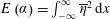 $E\left(\unicode[STIX]{x1D6FC}\right)=\int _{-\infty }^{\infty }\overline{\unicode[STIX]{x1D702}}^{2}\,\text{d}x$
. There is instability for
$E\left(\unicode[STIX]{x1D6FC}\right)=\int _{-\infty }^{\infty }\overline{\unicode[STIX]{x1D702}}^{2}\,\text{d}x$
. There is instability for
 $\unicode[STIX]{x1D706}^{(1)^{2}}>0$
. Turning our attention to the integral on the right-hand side, let the Fourier transform of
$\unicode[STIX]{x1D706}^{(1)^{2}}>0$
. Turning our attention to the integral on the right-hand side, let the Fourier transform of
 $\overline{\unicode[STIX]{x1D702}}(x)$
be
$\overline{\unicode[STIX]{x1D702}}(x)$
be
 $$\begin{eqnarray}\mathscr{F}\left\{\overline{\unicode[STIX]{x1D702}}(x)\right\}=\frac{1}{2\unicode[STIX]{x03C0}}\int _{-\infty }^{\infty }\overline{\unicode[STIX]{x1D702}}(x)\text{e}^{-\text{i}kx}\,\text{d}x=Y(k).\end{eqnarray}$$
Then, the Fourier transform of
 $\mathscr{H}\left\{\overline{\unicode[STIX]{x1D702}}_{x}\right\}$
is expressed as follows:
$\mathscr{H}\left\{\overline{\unicode[STIX]{x1D702}}_{x}\right\}$
is expressed as follows:
 $$\begin{eqnarray}\mathscr{F}\left\{\mathscr{H}\{\overline{\unicode[STIX]{x1D702}}_{x}\}\right\}=-\text{i}\text{sgn}(k)\mathscr{F}\left\{\overline{\unicode[STIX]{x1D702}}_{x}\right\}=-\text{i}\text{sgn}(k)(\text{i}k)\mathscr{F}\left\{\overline{\unicode[STIX]{x1D702}}\right\}=|k|Y(k).\end{eqnarray}$$
Then, using the following Parseval or Plancherel theorem,
 $$\begin{eqnarray}\int _{-\infty }^{\infty }f(x)g(x)\,\text{d}x=\frac{1}{2\unicode[STIX]{x03C0}}\int _{-\infty }^{\infty }F(-k)G(k)\,\text{d}k.\end{eqnarray}$$
The integral on the right-hand side in (6.27) becomes
 $$\begin{eqnarray}\int _{-\infty }^{\infty }\overline{\unicode[STIX]{x1D702}}\mathscr{H}\{\overline{\unicode[STIX]{x1D702}}_{x}\}\,\text{d}x=\frac{1}{2\unicode[STIX]{x03C0}}\int _{-\infty }^{\infty }Y(-k)|k|Y(k)\,\text{d}k.\end{eqnarray}$$
Since
 $\overline{\unicode[STIX]{x1D702}}(x)$
is real and even (6.2), the Fourier transform of it is also real and even,
$\overline{\unicode[STIX]{x1D702}}(x)$
is real and even (6.2), the Fourier transform of it is also real and even,
 $$\begin{eqnarray}Y(k)=Y(-k).\end{eqnarray}$$
Then, (6.31) becomes
 $$\begin{eqnarray}\int _{-\infty }^{\infty }\overline{\unicode[STIX]{x1D702}}\mathscr{H}\{\overline{\unicode[STIX]{x1D702}}_{x}\}\,\text{d}x=\frac{1}{2\unicode[STIX]{x03C0}}\int _{-\infty }^{\infty }|k|Y^{2}(k)\,\text{d}k>0.\end{eqnarray}$$
Finally, from (6.27) and (6.33), there is instability if
 $$\begin{eqnarray}\frac{\unicode[STIX]{x2202}E}{\unicode[STIX]{x2202}\unicode[STIX]{x1D6FC}}<0.\end{eqnarray}$$
Figure 25. The numerically obtained dimensionless energy (
 $E=\int _{-\infty }^{\infty }\overline{\unicode[STIX]{x1D702}}^{2}\,\text{d}x$
) of the 2-D gravity–capillary solitary waves according to the wave speed
$E=\int _{-\infty }^{\infty }\overline{\unicode[STIX]{x1D702}}^{2}\,\text{d}x$
) of the 2-D gravity–capillary solitary waves according to the wave speed
 $\unicode[STIX]{x1D6FC}$
from (6.1).
$\unicode[STIX]{x1D6FC}$
from (6.1).
This is the transverse instability condition, which is mentioned in the introduction. Therefore, we have proved that 2-D gravity–capillary solitary waves on deep water are unstable to transverse perturbations. Equation (6.34) is also numerically verified by solving (6.1), and the results are shown in figure 25. The present linear stability analysis is used to show the onset of the observed transverse instability of the present experiment with a long-wave perturbation with dimensionless wavenumber
 $\unicode[STIX]{x1D707}=1/6\ll 1$
, or dimensionally
$\unicode[STIX]{x1D707}=1/6\ll 1$
, or dimensionally
 $\unicode[STIX]{x1D707}/L_{char}=2\unicode[STIX]{x03C0}/w=0.06$
(
$\unicode[STIX]{x1D707}/L_{char}=2\unicode[STIX]{x03C0}/w=0.06$
(
 $1~\text{mm}^{-1}$
), where
$1~\text{mm}^{-1}$
), where
 $L_{char}=2.73$
mm. What happens really (nonlinearly) after the onset of instability was shown using a full numerical simulation in § 5. The sinusoidal perturbation is triggered as a single-wavelength mode of the natural transverse modes (
$L_{char}=2.73$
mm. What happens really (nonlinearly) after the onset of instability was shown using a full numerical simulation in § 5. The sinusoidal perturbation is triggered as a single-wavelength mode of the natural transverse modes (
 $m\unicode[STIX]{x03C0}/w$
,
$m\unicode[STIX]{x03C0}/w$
,
 $m=2$
) due to the existence of sidewalls in the present box-shaped experimental setting (width
$m=2$
) due to the existence of sidewalls in the present box-shaped experimental setting (width
 $w=100$
mm). Physically, this sinusoidal perturbation with a long wavelength (
$w=100$
mm). Physically, this sinusoidal perturbation with a long wavelength (
 $100~\text{mm}\gg 2.73~\text{mm}$
) will be a standing gravity wave in a potential flow. Therefore, the wall boundary conditions will be zero normal velocity components as are usually adopted in potential-flow analysis. In the above linear stability analysis and nonlinear numerical simulation in § 5, we assumed that, initially, the transverse perturbation exists due to the existence of sidewalls. Therefore, we did not explicitly use the velocity-related boundary conditions, and, instead, a periodic boundary condition for the existence of a sinusoidal perturbation was adopted. Similar kinds of long-wave transverse instability analysis and relevant simulations using a single-wavelength perturbation have been carried out for gravity–capillary interfacial waves between two fluids (Kim & Akylas Reference Kim and Akylas2006) and gravity–capillary surface waves on deep water (Akers & Milewski Reference Akers and Milewski2009; Wang & Vanden-Broeck (Reference Wang and Vanden-Broeck2015)). We also would like to mention that the stability/instability in the present work (and other referenced works) means stable/unstable behaviour of a gravity–capillary wave after a perturbation is uncontrollably generated internally (like a long-time experiment or simulation) or given externally (like the present experiment or simulation). In addition, the stability analysis here focuses on one mode of instability (
$100~\text{mm}\gg 2.73~\text{mm}$
) will be a standing gravity wave in a potential flow. Therefore, the wall boundary conditions will be zero normal velocity components as are usually adopted in potential-flow analysis. In the above linear stability analysis and nonlinear numerical simulation in § 5, we assumed that, initially, the transverse perturbation exists due to the existence of sidewalls. Therefore, we did not explicitly use the velocity-related boundary conditions, and, instead, a periodic boundary condition for the existence of a sinusoidal perturbation was adopted. Similar kinds of long-wave transverse instability analysis and relevant simulations using a single-wavelength perturbation have been carried out for gravity–capillary interfacial waves between two fluids (Kim & Akylas Reference Kim and Akylas2006) and gravity–capillary surface waves on deep water (Akers & Milewski Reference Akers and Milewski2009; Wang & Vanden-Broeck (Reference Wang and Vanden-Broeck2015)). We also would like to mention that the stability/instability in the present work (and other referenced works) means stable/unstable behaviour of a gravity–capillary wave after a perturbation is uncontrollably generated internally (like a long-time experiment or simulation) or given externally (like the present experiment or simulation). In addition, the stability analysis here focuses on one mode of instability (
 $\unicode[STIX]{x1D707}=1/6\ll 1$
) and not on the whole spectrum.
$\unicode[STIX]{x1D707}=1/6\ll 1$
) and not on the whole spectrum.
7 Summary
The generation of two-dimensional (2-D) gravity–capillary solitary waves on deep water and their transverse instability were investigated experimentally and confirmed numerically using a theoretical model equation that admits gravity–capillary solitary wave solutions near the minimum of the phase speed
 $c_{min}$
of linear gravity–capillary waves on deep water. In the experiment, we generated 2-D depression gravity–capillary solitary waves using a moving pressure jet from a narrow slit as a forcing onto the free surface of deep water, and observed the transverse instability of 2-D depression gravity–capillary solitary waves and the resultant formation of 3-D depression gravity–capillary solitary waves. These experimental observations were compared with numerical results based on a model equation and they agree with each other very well. Based on a linear stability analysis using the same model equation, we also provided a theoretically complete proof for the observed transverse instability of 2-D depression gravity–capillary solitary waves, i.e.
$c_{min}$
of linear gravity–capillary waves on deep water. In the experiment, we generated 2-D depression gravity–capillary solitary waves using a moving pressure jet from a narrow slit as a forcing onto the free surface of deep water, and observed the transverse instability of 2-D depression gravity–capillary solitary waves and the resultant formation of 3-D depression gravity–capillary solitary waves. These experimental observations were compared with numerical results based on a model equation and they agree with each other very well. Based on a linear stability analysis using the same model equation, we also provided a theoretically complete proof for the observed transverse instability of 2-D depression gravity–capillary solitary waves, i.e.
 $\unicode[STIX]{x2202}E/\unicode[STIX]{x2202}c<0$
.
$\unicode[STIX]{x2202}E/\unicode[STIX]{x2202}c<0$
.
Acknowledgement
This work was supported by the National Research Foundation of Korea (NRF) (NRF-2017R1D1A1B03028299).
Appendix A. Derivation of (3.1) (Cho et al. Reference Cho, Diorio, Akylas and Duncan2011; Cho Reference Cho2014; Park & Cho Reference Park and Cho2016)
From the inviscid dispersion relation of the potential-flow theory for linear sinusoidal gravity–capillary waves on deep water,
 $$\begin{eqnarray}\unicode[STIX]{x1D714}^{2}=g\unicode[STIX]{x1D705}+\frac{\unicode[STIX]{x1D70E}}{\unicode[STIX]{x1D70C}}\unicode[STIX]{x1D73F}^{3},\end{eqnarray}$$
where
 $\unicode[STIX]{x1D714}$
is the angular frequency,
$\unicode[STIX]{x1D714}$
is the angular frequency,
 $g$
is the gravitational acceleration,
$g$
is the gravitational acceleration,
 $\unicode[STIX]{x1D73F}$
is the magnitude of the wavenumber vector
$\unicode[STIX]{x1D73F}$
is the magnitude of the wavenumber vector
 $\unicode[STIX]{x1D73F}=\sqrt{k^{2}+l^{2}}$
,
$\unicode[STIX]{x1D73F}=\sqrt{k^{2}+l^{2}}$
,
 $k$
is the wavenumber in the
$k$
is the wavenumber in the
 $x$
direction,
$x$
direction,
 $l$
is the wavenumber in the
$l$
is the wavenumber in the
 $y$
direction,
$y$
direction,
 $\unicode[STIX]{x1D70E}$
is the coefficient of surface tension and
$\unicode[STIX]{x1D70E}$
is the coefficient of surface tension and
 $\unicode[STIX]{x1D70C}$
is the fluid density. Assuming a linear wave propagating in the positive or negative
$\unicode[STIX]{x1D70C}$
is the fluid density. Assuming a linear wave propagating in the positive or negative
 $x$
direction, the phase speed
$x$
direction, the phase speed
 $c=\pm \text{sgn}(k)\unicode[STIX]{x1D714}/\unicode[STIX]{x1D73F}$
features a minimum
$c=\pm \text{sgn}(k)\unicode[STIX]{x1D714}/\unicode[STIX]{x1D73F}$
features a minimum
 $c_{min}$
at a non-zero finite wavenumber
$c_{min}$
at a non-zero finite wavenumber
 $(k,l)=(\pm \sqrt{\unicode[STIX]{x1D70C}g/\unicode[STIX]{x1D70E}},0)$
. Using the length scale
$(k,l)=(\pm \sqrt{\unicode[STIX]{x1D70C}g/\unicode[STIX]{x1D70E}},0)$
. Using the length scale
 $\sqrt{\unicode[STIX]{x1D70E}/\unicode[STIX]{x1D70C}g}$
and the time scale
$\sqrt{\unicode[STIX]{x1D70E}/\unicode[STIX]{x1D70C}g}$
and the time scale
 $\sqrt{\unicode[STIX]{x1D70E}/\unicode[STIX]{x1D70C}g}/c_{min}$
, the dispersion relation (A 1) becomes dimensionless,
$\sqrt{\unicode[STIX]{x1D70E}/\unicode[STIX]{x1D70C}g}/c_{min}$
, the dispersion relation (A 1) becomes dimensionless,
 $$\begin{eqnarray}\unicode[STIX]{x1D714}^{2}={\textstyle \frac{1}{2}}(\unicode[STIX]{x1D73F}+\unicode[STIX]{x1D73F}^{3}),\end{eqnarray}$$
and the phase-speed minimum becomes
 $c_{min}=1$
at
$c_{min}=1$
at
 $(k,l)=(k_{m},l_{m})=(\pm 1,0)$
. To capture the essential wave phenomena near the minimum phase speed
$(k,l)=(k_{m},l_{m})=(\pm 1,0)$
. To capture the essential wave phenomena near the minimum phase speed
 $c_{min}$
, (A 2) is Taylor-expanded around
$c_{min}$
, (A 2) is Taylor-expanded around
 $(k,l)=(k_{m},l_{m})$
(Akers & Milewski Reference Akers and Milewski2009; Diorio et al.
Reference Diorio, Cho, Duncan and Akylas2009; Cho et al.
Reference Cho, Diorio, Akylas and Duncan2011; Cho Reference Cho2014),
$(k,l)=(k_{m},l_{m})$
(Akers & Milewski Reference Akers and Milewski2009; Diorio et al.
Reference Diorio, Cho, Duncan and Akylas2009; Cho et al.
Reference Cho, Diorio, Akylas and Duncan2011; Cho Reference Cho2014),
 $$\begin{eqnarray}\displaystyle \unicode[STIX]{x1D714}(k,l) & = & \displaystyle \pm \text{sgn}(k)\sqrt{{\displaystyle \frac{1}{2}}(\unicode[STIX]{x1D73F}+\unicode[STIX]{x1D73F}^{3})}=\pm ~\text{sgn}(k)\sqrt{{\displaystyle \frac{1}{2}}}\sqrt{(k^{2}+l^{2})^{1/2}+(k^{2}+l^{2})^{3/2}}\nonumber\\ \displaystyle & {\approx} & \displaystyle \pm \text{sgn}(k)\left\{\unicode[STIX]{x1D714}(k_{m},l_{m})+\frac{\unicode[STIX]{x2202}\unicode[STIX]{x1D714}}{\unicode[STIX]{x2202}k}\bigg|_{m}(k-k_{m})+\frac{\unicode[STIX]{x2202}\unicode[STIX]{x1D714}}{\unicode[STIX]{x2202}l}\bigg|_{m}(l-l_{m})\quad \;\;\right.\nonumber\\ \displaystyle & & \displaystyle \left.\text{}+\,\frac{\unicode[STIX]{x2202}^{2}\unicode[STIX]{x1D714}}{\unicode[STIX]{x2202}k^{2}}\bigg|_{m}(k-k_{m})^{2}+2\frac{\unicode[STIX]{x2202}^{2}\unicode[STIX]{x1D714}}{\unicode[STIX]{x2202}k\unicode[STIX]{x2202}l}\bigg|_{m}(k-k_{m})(l-l_{m})+\frac{\unicode[STIX]{x2202}^{2}\unicode[STIX]{x1D714}}{\unicode[STIX]{x2202}l^{2}}\bigg|_{m}(l-l_{m})^{2}\right\}\nonumber\\ \displaystyle & = & \displaystyle \pm \frac{1}{4}\text{sgn}(k)(1+2|k|+k^{2}+2l^{2}).\end{eqnarray}$$
Assuming a left-going wave, the linear dispersion relation is
 $$\begin{eqnarray}\unicode[STIX]{x1D714}=-{\textstyle \frac{1}{4}}\text{sgn}(k)(1+2|k|+k^{2}+2l^{2}).\end{eqnarray}$$
The viscous effect can be reflected in the inviscid dispersion relation as follows:
 $$\begin{eqnarray}\unicode[STIX]{x1D714}=-{\textstyle \frac{1}{4}}\text{sgn}(k)(1+2|k|+k^{2}+2l^{2})-\text{i}\widetilde{\unicode[STIX]{x1D708}}|k|^{2}.\end{eqnarray}$$
Here,
 $\widetilde{\unicode[STIX]{x1D708}}=C\unicode[STIX]{x1D708}(4g)^{1/4}(\unicode[STIX]{x1D70C}/\unicode[STIX]{x1D70E})^{3/4}$
is the dimensionless kinematic viscosity, where
$\widetilde{\unicode[STIX]{x1D708}}=C\unicode[STIX]{x1D708}(4g)^{1/4}(\unicode[STIX]{x1D70C}/\unicode[STIX]{x1D70E})^{3/4}$
is the dimensionless kinematic viscosity, where
 $\unicode[STIX]{x1D708}=10^{-6}~(\text{m}^{2}~\text{s}^{-1})$
is the kinematic viscosity of water and
$\unicode[STIX]{x1D708}=10^{-6}~(\text{m}^{2}~\text{s}^{-1})$
is the kinematic viscosity of water and
 $C$
is the parameter (
$C$
is the parameter (
 $C=1$
for linear sinusoidal waves,
$C=1$
for linear sinusoidal waves,
 $C>1$
for nonlinear solitary waves) that determines the decay rate of waves (Longuet-Higgins Reference Longuet-Higgins1997).
$C>1$
for nonlinear solitary waves) that determines the decay rate of waves (Longuet-Higgins Reference Longuet-Higgins1997).
Now, from (A 5), one can replace variables (
 $\unicode[STIX]{x1D714},k,l$
) in the temporal and spatial frequency domains with those (
$\unicode[STIX]{x1D714},k,l$
) in the temporal and spatial frequency domains with those (
 $t,x,y$
) in the physical domain,
$t,x,y$
) in the physical domain,
 $$\begin{eqnarray}\unicode[STIX]{x1D714}\rightarrow \text{i}\frac{\unicode[STIX]{x2202}}{\unicode[STIX]{x2202}t},\quad k\rightarrow -\text{i}\frac{\unicode[STIX]{x2202}}{\unicode[STIX]{x2202}x},\quad l\rightarrow -\text{i}\frac{\unicode[STIX]{x2202}}{\unicode[STIX]{x2202}y},\quad \text{sgn}(k)\rightarrow -\text{i}\mathscr{H},\end{eqnarray}$$
where
 $\mathscr{H}\{f\}=\mathscr{F}^{-1}\{-\text{i}\text{sgn}(k)\mathscr{F}\{f\}\}$
stands for the Hilbert transform, with
$\mathscr{H}\{f\}=\mathscr{F}^{-1}\{-\text{i}\text{sgn}(k)\mathscr{F}\{f\}\}$
stands for the Hilbert transform, with
 $$\begin{eqnarray}\mathscr{F}\left\{f\right\}=\frac{1}{2}\int _{-\infty }^{\infty }f(x)\text{e}^{-\text{i}kx}\,\text{d}x\end{eqnarray}$$
being the Fourier transform. Consequently, one obtains the following model equation for linear gravity–capillary waves on deep water:
 $$\begin{eqnarray}\unicode[STIX]{x1D702}_{t}-\widetilde{\unicode[STIX]{x1D708}}(\unicode[STIX]{x1D702}_{xx}+\unicode[STIX]{x1D702}_{yy})-{\textstyle \frac{1}{2}}\unicode[STIX]{x1D702}_{x}-{\textstyle \frac{1}{4}}\mathscr{H}\left\{\unicode[STIX]{x1D702}_{xx}+2\unicode[STIX]{x1D702}_{yy}-\unicode[STIX]{x1D702}\right\}=0,\end{eqnarray}$$
where
 $\unicode[STIX]{x1D702}=\unicode[STIX]{x1D702}(x,y,t)$
is the wave elevation and the subscript denotes partial differentiation. To account for the nonlinearity and the left-moving forcing, one can add a quadratic nonlinearity term
$\unicode[STIX]{x1D702}=\unicode[STIX]{x1D702}(x,y,t)$
is the wave elevation and the subscript denotes partial differentiation. To account for the nonlinearity and the left-moving forcing, one can add a quadratic nonlinearity term
 $\unicode[STIX]{x1D6FD}(\unicode[STIX]{x1D702}^{2})_{x}$
and the forcing
$\unicode[STIX]{x1D6FD}(\unicode[STIX]{x1D702}^{2})_{x}$
and the forcing
 $Ap(x+\unicode[STIX]{x1D6FC}t)$
in the equation,
$Ap(x+\unicode[STIX]{x1D6FC}t)$
in the equation,
 $$\begin{eqnarray}\unicode[STIX]{x1D702}_{t}-\widetilde{\unicode[STIX]{x1D708}}(\unicode[STIX]{x1D702}_{xx}+\unicode[STIX]{x1D702}_{yy})-{\textstyle \frac{1}{2}}\unicode[STIX]{x1D702}_{x}-\unicode[STIX]{x1D6FD}(\unicode[STIX]{x1D702}^{2})_{x}-{\textstyle \frac{1}{4}}\mathscr{H}\left\{\unicode[STIX]{x1D702}_{xx}+2\unicode[STIX]{x1D702}_{yy}-\unicode[STIX]{x1D702}\right\}=Ap_{x}(x+\unicode[STIX]{x1D6FC}t).\end{eqnarray}$$
By replacing
 $x$
with
$x$
with
 $x+\unicode[STIX]{x1D6FC}t$
in (A 9), the wave equation, which is expressed in the left-moving frame of reference with a dimensionless speed
$x+\unicode[STIX]{x1D6FC}t$
in (A 9), the wave equation, which is expressed in the left-moving frame of reference with a dimensionless speed
 $\unicode[STIX]{x1D6FC}=U/c_{min}$
, is obtained as follows:
$\unicode[STIX]{x1D6FC}=U/c_{min}$
, is obtained as follows:
 $$\begin{eqnarray}\unicode[STIX]{x1D702}_{t}-\widetilde{\unicode[STIX]{x1D708}}(\unicode[STIX]{x1D702}_{xx}+\unicode[STIX]{x1D702}_{yy})+(\unicode[STIX]{x1D6FC}-{\textstyle \frac{1}{2}})\unicode[STIX]{x1D702}_{x}-\unicode[STIX]{x1D6FD}(\unicode[STIX]{x1D702}^{2})_{x}-{\textstyle \frac{1}{4}}\mathscr{H}\left\{\unicode[STIX]{x1D702}_{xx}+2\unicode[STIX]{x1D702}_{yy}-\unicode[STIX]{x1D702}\right\}=Ap_{x}(x).\end{eqnarray}$$
To determine the nonlinear coefficient
 $\unicode[STIX]{x1D6FD}$
, one can consider the following inviscid forcing-free model equation from (A 10):
$\unicode[STIX]{x1D6FD}$
, one can consider the following inviscid forcing-free model equation from (A 10):
 $$\begin{eqnarray}\unicode[STIX]{x1D702}_{t}+(\unicode[STIX]{x1D6FC}-{\textstyle \frac{1}{2}})\unicode[STIX]{x1D702}_{x}-\unicode[STIX]{x1D6FD}(\unicode[STIX]{x1D702}^{2})_{x}-{\textstyle \frac{1}{4}}\mathscr{H}\{\unicode[STIX]{x1D702}_{xx}+2\unicode[STIX]{x1D702}_{yy}-\unicode[STIX]{x1D702}\}=0.\end{eqnarray}$$
In the weakly nonlinear small-amplitude limit near
 $\unicode[STIX]{x1D6FC}=1$
, the solution to (A 11) can be expressed as
$\unicode[STIX]{x1D6FC}=1$
, the solution to (A 11) can be expressed as
 $$\begin{eqnarray}\unicode[STIX]{x1D702}={\textstyle \frac{1}{2}}\unicode[STIX]{x1D716}\{S(X,Y)\text{e}^{\text{i}x}+\text{c.c.}\}+{\textstyle \frac{1}{2}}\unicode[STIX]{x1D716}^{2}\{S_{2}(X,Y)\text{e}^{2\text{i}x}+\text{c.c.}\}+\cdots \,,\end{eqnarray}$$
where
 $\unicode[STIX]{x1D6FC}=1-\unicode[STIX]{x1D716}^{2}(0<\unicode[STIX]{x1D716}\ll 1)$
and
$\unicode[STIX]{x1D6FC}=1-\unicode[STIX]{x1D716}^{2}(0<\unicode[STIX]{x1D716}\ll 1)$
and
 $(X,Y)=\unicode[STIX]{x1D716}(x,y)$
. Substituting (A 12) into (A 11), one obtains the following nonlinear Schrödinger (NLS) equation:
$(X,Y)=\unicode[STIX]{x1D716}(x,y)$
. Substituting (A 12) into (A 11), one obtains the following nonlinear Schrödinger (NLS) equation:
 $$\begin{eqnarray}-S+{\textstyle \frac{1}{4}}S_{XX}+{\textstyle \frac{1}{2}}S_{YY}+4\unicode[STIX]{x1D6FD}^{2}|S|^{2}S=0.\end{eqnarray}$$
On the other hand, from the full water-wave or Euler equations on deep water, the NLS equation is derived as (Hogan Reference Hogan1985)
 $$\begin{eqnarray}-S+{\textstyle \frac{1}{4}}S_{XX}+{\textstyle \frac{1}{2}}S_{YY}+{\textstyle \frac{11}{32}}|S|^{2}S=0.\end{eqnarray}$$
Finally, by equating (A 13) and (A 14), the nonlinear coefficient is determined as
 $\unicode[STIX]{x1D6FD}=\sqrt{11/2}/8$
.
$\unicode[STIX]{x1D6FD}=\sqrt{11/2}/8$
.


