2.1. The governing equations

The granular material is treated as the bulk fluid with the bulk density defined asρ = φρ_s, whereφ is the volume fraction and ρ_s is the density of the grains. In granular column collapse, the volume fraction has a small variation in the range 0.59–0.65 (Lajeunesse et al. Reference Lajeunesse, Mangeney-Castelnau and Vilotte2004; Lajeunesse et al. Reference Lajeunesse, Monnier and Homsy2005), so φ is assumed to be constant as φ = 0.62, which results in a constant bulk density. Thus, the bulk fluid for the granular material is modelled as an incompressible fluid, with the governing equations in the Lagrangian framework expressed as (Minatti & Paris Reference Minatti and Paris2015; Xu et al. Reference Xu, Jin and Tai2019)

(2.1)\begin{gather}\boldsymbol{\nabla }\boldsymbol{\cdot }\boldsymbol{u} = 0,\end{gather}

(2.2)\begin{gather}\rho \frac{{\textrm{D}\boldsymbol{u}}}{{\textrm{D}t}} ={-} \boldsymbol{\nabla }p + \boldsymbol{\nabla }\boldsymbol{\cdot }\boldsymbol{\tau } + \rho \boldsymbol{g},\end{gather}

where t is the time, u is the velocity vector, p is the pressure, τ is the deviatoric shear stress $\boldsymbol{\tau } = \eta \gamma$ (γ is the strain rate tensor), g is the external force such as gravity and D/Dt indicates the Lagrangian derivative operator. To calculate the continuity condition, an equation of state is used, and the incompressible fluid is assumed to be weakly compressible with a compressibility of less than 1 %.

2.2. Mesh-free discretization

The spatial operators are adopted in the framework of the MPS (Koshizuka et al. Reference Koshizuka, Nobe and Oka1998; Gotoh & Khayyer Reference Gotoh and Khayyer2016; Xu & Jin Reference Xu and Jin2016a). By using the mesh-free method, the granular material is represented by a set of Lagrangian particles with the same initial distance Δl, being the continuum-level markers. Similarly, the solid boundary to confine the granular material is also discretized into the particles with the same distance Δl. The interaction between these Lagrangian particles is realized by using a weighting function and the weighting function w_ij used in this study is expressed as (Shakibaeinia & Jin Reference Shakibaeinia and Jin2010)

(2.3)\begin{equation}{w_{ij}} = w({r_{ij}},{r_e}) = \left\{ {\begin{array}{@{}ll} {{{\left( {1 - \dfrac{{{r_{ij}}}}{{{r_e}}}} \right)}^3}}&{{r_{ij}} \le {r_e}}\\ 0&{{r_{ij}} \gt {r_e}} \end{array}} \right..\end{equation}

The weighting function constitutes the interaction radius r_e and the distance r_ij between two Lagrangian particles indexed by i and j. The interaction radius r_e determines the interaction circle in two dimensions, which marks the neighbouring particles j for the target particle i according to the distance r_ij. For the neighbouring particles j at r_ij > r_e, their interaction to particle i is assumed to be negligible. This enables an avoidance of the calculation of all the Lagrangian particles in the whole domain when calculating the information of the target particle i. The interaction radius r_e is usually related to the discretized particle distance Δl, so that the number of neighbouring particles j can be effectively and efficiently identified. The spatial operators in the method, such as the gradient, divergence and Laplacian models, were developed by counting contributions from the neighbouring particles with the weighting function. A large r_e can involve a large number of neighbouring particles j, which can improve the accuracy for the spatial operator calculation but reduce the computing efficiency. For a small r_e, the number of neighbouring particles and computational cost can be reduced but the accuracy is eliminated. To balance between accuracy and efficiency, the interaction radius is usually set to be r_e = (3.0–4.0)Δl in the previous studies (Monaghan Reference Monaghan1994; Koshizuka et al. Reference Koshizuka, Nobe and Oka1998; Lee et al. Reference Lee, Park, Kim and Hwang2011; Gotoh & Khayyer Reference Gotoh and Khayyer2016; Violeau & Rogers Reference Violeau and Rogers2016; Xu & Jin Reference Xu and Jin2016a).

In the MPS method, the particle number density is defined as the summation of the weighting function as (Koshizuka et al. Reference Koshizuka, Nobe and Oka1998)

(2.4)\begin{equation}{N_i} = \mathop \sum \limits_{j \ne i} {w_{ij}}.\end{equation}

The number of particles in a unit volume ρ_n can be approximated by the particle number density as (Koshizuka et al. Reference Koshizuka, Nobe and Oka1998)

(2.5)\begin{equation}{\rho _n} = \frac{{{N_i}}}{{\int {w\,\textrm{d}V} }},\end{equation}

where the integration at the right-hand side for the weighting function is over the entire domain and the integration is constant for a fixed interaction radius r_e. Thus, the fluid density can be expressed as

(2.6)\begin{equation}{\rho _i} = m{\rho _n} = \frac{{m{N_i}}}{{\int {w\,\textrm{d}V} }},\end{equation}

where m represents the mass that a particle takes. Equation (2.6) indicates that the fluid density is proportional to the particle number density N_i, which can be used in the equation of state to calculate the pressure field.

When the interaction circle for the weighting function is full of Lagrangian particles with the same distance Δl, the particle number density is referred to as the initial particle number density N ₀. It is constant throughout the calculation.

The spatial operator to calculate the gradient is written as (Koshizuka et al. Reference Koshizuka, Nobe and Oka1998)

(2.7)\begin{equation}\langle \boldsymbol{\nabla }{\phi _i}\rangle = \frac{{{D_m}}}{{{N_0}}}\mathop \sum \limits_{j \ne i} \frac{{{\phi _j} - {\phi _i}}}{{r_{ij}^2}}{\boldsymbol{r}_{ij}}{w_{ij}},\end{equation}

where ϕ is a scalar, D_m is the dimension of space and r_ij is the vector from particle i to particle j. This gradient model is used to calculate the shear rate and the velocity gradient in the proposed numerical scheme, and the interaction radius is defined as ${r_e} = 4.0\Delta l$ to ensure its accuracy.

To calculate the pressure, an equation of state is employed, and the granular flow is assumed to be weakly compressible. The equation of state based on the particle number density is expressed as (Shakibaeinia & Jin Reference Shakibaeinia and Jin2010; Xu & Jin Reference Xu and Jin2016a)

(2.8)\begin{equation}{p_i} = \frac{{\rho c_0^2}}{\lambda }\left( {{{\left( {\frac{{{N_i}}}{{{N_0}}}} \right)}^\lambda } - 1} \right),\end{equation}

where λ = 7, according to the previous studies (Monaghan Reference Monaghan1994; Shakibaeinia & Jin Reference Shakibaeinia and Jin2010; González-Cao et al. Reference González-Cao, Altomare, Crespo, Domínguez, Gómez-Gesteira and Kisacik2019), and c ₀ is the artificial speed of sound. The value of c ₀ sets a requirement for the time step in the simulation. A much larger c ₀ means that a much smaller time step should be implemented by using the equation of state. Here, c ₀ also determines the compressibility when modelling the incompressible fluid flow. To balance between the time step and the compressibility for modelling the incompressible fluid, c ₀ is defined as 10 times the maximum velocity in the problem (Monaghan Reference Monaghan1994; Violeau & Rogers Reference Violeau and Rogers2016; González-Cao et al. Reference González-Cao, Altomare, Crespo, Domínguez, Gómez-Gesteira and Kisacik2019). This can limit the compressibility for the modelled incompressible fluid to within 1 % with an acceptable time step (Monaghan Reference Monaghan1994). Velocity in the solid-like state for the granular flow is very small and defining c ₀ 10 times the maximum velocity is sufficient to ensure the incompressibility for the flow. In this study, the time step satisfies the Courant–Friedrichs–Lewy condition (Shadloo et al. Reference Shadloo, Zainali, Yildiz and Suleman2012).

The mesh-free method is based on the Lagrangian approach, which updates the positions of the Lagrangian particles in each time step. However, during the movement of particles, some particles can approach each other making their distance much shorter than the initial distance Δl. If there is no numerical technique to prevent further joining, clustering of particles can occur, which results in an instability for the calculation. To solve this problem, a collision model is proposed to keep particles from clustering in the simulation (Lee et al. Reference Lee, Park, Kim and Hwang2011). When the distance between two particles r_ij is shorter than a threshold, the collision is activated to maintain the particle distance. The threshold is defined as the collision distance, which is equal to d_coll = (0.85–0.95)Δl according to the previous studies (Lee et al. Reference Lee, Park, Kim and Hwang2011; Shakibaeinia & Jin Reference Shakibaeinia and Jin2012), and d_coll = 0.9Δl is selected in this study. The collision model is expressed as (Shakibaeinia & Jin Reference Shakibaeinia and Jin2012)

(2.9)\begin{equation}\left\{ {\begin{array}{@{}ll} {\boldsymbol{u}_i^{new} = {\boldsymbol{u}_i} - {\textstyle{1 \over 2}}u_{ij}^{/{/}}{\boldsymbol{e}_{ij}}}\\ {\boldsymbol{u}_j^{new} = {\boldsymbol{u}_j} - {\textstyle{1 \over 2}}u_{ij}^{/{/}}{\boldsymbol{e}_{ij}}} \end{array}} \right.\quad {r_{ij}} \lt 0.9\Delta l,\end{equation}

where $u_{ij}^{/{/}}$ is the approaching velocity between particles i and j, and e_ij is the unit vector to project the approaching velocity $u_{ij}^{/{/}}$ to the vectors u_i and u_j.

The positions of the two particles i and j are updated according to the collision velocity as

(2.10)\begin{equation}\left\{ {\begin{array}{@{}ll} {\boldsymbol{r}_i^{new} = {\boldsymbol{r}_i} - {\textstyle{1 \over 2}}u_{ij}^{/{/}}{\boldsymbol{e}_{ij}}\Delta t}\\ {\boldsymbol{r}_j^{new} = {\boldsymbol{r}_j} - {\textstyle{1 \over 2}}u_{ij}^{/{/}}{\boldsymbol{e}_{ij}}\Delta t} \end{array}} \right.\quad {r_{ij}} \lt 0.9\Delta l.\end{equation}

The free surface is recognized by the particle number density. When N_i is less than N ₀, particle i is regarded as a free surface particle with zero pressure prescribed. The solid boundary is discretized into a set of particles with the same distance Δl. However, when using the spatial operator of the gradient model to calculate the shear rate and velocity gradient for a 2-D problem, the local interaction circle in the vicinity of the solid boundary is partially filled with particles. The area for the interaction circle beyond the solid boundary is empty. This can result in an inaccuracy when calculating the spatial operator. The problem also occurs when calculating the particle number density using (2.4). To offset the deficiency of the particles for the interaction circle close to the boundary, several layers of ghost particles are set-up beyond the solid boundary. The number of layers for the ghost particles is dependent on the interaction radius r_e, for example, for r_e = 4.0Δl, four layers of ghost particles are required to make the interaction circle full of particles. The flow properties of these ghost particles, such as velocity and pressure, are set to be the same as their solid particles. This solid boundary treatment has been implemented in many applications by the mesh-free method with good numerical results achieved (Koshizuka et al. Reference Koshizuka, Nobe and Oka1998; Ye et al. Reference Ye, Pan, Huang and Liu2019).

3.1. The rheological law

In the mesh-free method, a set of Lagrangian particles are used to represent the granular material, which carry the properties of density, velocity, stress, viscosity and so forth. The viscosity for the granular flow is not constant, which has a large variation in space and time (Da Cruz et al. Reference Da Cruz, Emam, Prochnow, Roux and Chevoir2005). In this study, the μ(I) rheology, developed by MiDi (Reference MiDi2004) and generalized into a tensorial version by Jop et al. (Reference Jop, Forterre and Pouliquen2006), is used to calculate the effective viscosity and stress in the granular flow. In the model, the friction μ is expressed as (MiDi Reference MiDi2004; Da Cruz et al. Reference Da Cruz, Emam, Prochnow, Roux and Chevoir2005)

(3.1)\begin{equation}\mu (I) = {\mu _s} + \frac{{{\mu _2} - {\mu _s}}}{{{I_0}/I + 1}},\end{equation}

where I ₀ is a constant, μ is an increasing function with the dimensionless parameter I, bounded by μ_s at I = 0 and μ ₂ at high I. For glass beads, the parameters are μ_s = tan21°, μ ₂ = tan32° and I ₀ = 0.3 in the rheology (Jop Reference Jop2015).

The shear rate is calculated as

(3.2)\begin{gather}{\gamma _{\alpha \beta }} = \frac{1}{2}\left( {\frac{{\partial {u_\alpha }}}{{\partial {x_\beta }}} + \frac{{\partial {u_\beta }}}{{\partial {x_\alpha }}}} \right),\end{gather}

(3.3)\begin{gather}|\gamma |= \sqrt {0.5{\gamma _{\alpha \beta }}{\gamma _{\alpha \beta }}} ,\end{gather}

where α and β denote the coordinate components, and |γ| is the second invariant for the strain rate tensor.

The inertial number I is defined according to the simulation by Ionescu et al. (Reference Ionescu, Mangeney, Bouchut and Roche2015), which is modified from the definition by MiDi (Reference MiDi2004) and Jop et al. (Reference Jop, Forterre and Pouliquen2006) owing to the shear rate calculation in (3.2)

(3.4)\begin{equation}I = \frac{{2d|\gamma |}}{{\sqrt {p/{\rho _s}} }},\end{equation}

where d is the diameter of the grains.

The effective viscosity can be obtained by the friction, confining pressure and shear rate as (Jop et al. Reference Jop, Forterre and Pouliquen2006)

(3.5)\begin{equation}\eta = \frac{{\mu (I)p}}{{|\gamma |}}.\end{equation}

A regularization technique is applied to calculate the viscosity in (3.5) based on the inertial number I in (3.4) and friction μ in (3.1) as (Chauchat & Médale Reference Chauchat and Médale2014)

(3.6)\begin{equation}{\eta _r} = \left( {{\mu_s} + \frac{{2({\mu_2} - {\mu_s})|\gamma |}}{{{I_0}\sqrt {p/({\rho_s}{d^2})} + 2|\gamma |}}} \right)\frac{p}{{\sqrt {|\gamma {|^2} + {\delta ^2}} }},\end{equation}

where δ is a very small value. This regularization technique for the μ(I) rheology is proposed by Chauchat & Médale (Reference Chauchat and Médale2014) to avoid the infinite value for the viscosity in (3.5) when |γ| is approaching zero for p > 0.0. In their study (Chauchat & Médale Reference Chauchat and Médale2014), the parameter is tested in the range 10⁻⁶ < δ < 10⁻⁴ to simulate the vertical-chute flow and good numerical results are obtained. In simulating granular column collapse, we found the free surface and velocity show limited difference for 10⁻⁶ < δ < 10⁻⁴, and thus δ = 10⁻⁶ s⁻¹ is chosen in this study.

The rheological law expressed in (3.6) is a local model and its shortcoming includes the limitations in capturing the transition between the fluid-like and solid-like state (Jop et al. Reference Jop, Forterre and Pouliquen2006). As pointed out by Pouliquen & Forterre (Reference Pouliquen and Forterre2009), the quasi-static regime cannot be sufficiently reflected by the local model. However, to calculate the entire process for the collapse, the transition from the fluid-like to the solid-like state needs to be taken into consideration. Although many studies have been dedicated to developing the non-local rheological law (Pouliquen & Forterre Reference Pouliquen and Forterre2009; Bouzid et al. Reference Bouzid, Trulsson, Claudin, Clément and Andreotti2013, Reference Bouzid, Izzet, Trulsson, Clément, Claudin and Andreotti2015; Henann & Kamrin Reference Henann and Kamrin2013), reflecting the phase transition in the granular flow is still a challenge. However, peridynamics is a non-local theory which provides an approach to account for the interaction between grains.

3.2. Peridynamics

Peridynamics, as a generalization of the standard theory in solid mechanics, handles the mechanics with continuous bodies and discrete grains by including the long-range force (Silling & Askari Reference Silling and Askari2005; Silling et al. Reference Silling, Epton, Weckner, Xu and Askari2007; Silling & Lehoucq Reference Silling and Lehoucq2008; Mengesha & Du Reference Mengesha and Du2014; Ren et al. Reference Ren, Fan, Bergel, Regueiro, Lai and Li2015).

The integrated equation of motion in peridynamics is expressed as

(3.7)\begin{equation}\rho \ddot{\boldsymbol{r}} = \int_{{H_{\boldsymbol{x}}}} {\boldsymbol{F}(\boldsymbol{x},\boldsymbol{x^{\prime}},t)\,\textrm{d}{V_{\boldsymbol{x^{\prime}}}} + \rho \boldsymbol{g}} ,\end{equation}

where H _x is a neighbourhood of x, x′ is the displacement vector and F is a pairwise force.

(3.8)\begin{equation}\boldsymbol{F}(\boldsymbol{x},\boldsymbol{x^{\prime}},t) = \boldsymbol{T}(\boldsymbol{x},\boldsymbol{x^{\prime}} - \boldsymbol{x},t) - \boldsymbol{T}(\boldsymbol{x^{\prime}},\boldsymbol{x} - \boldsymbol{x^{\prime}},t),\end{equation}

where T is the force state.

The equation of motion in the discretized form for the target particle i with neighbouring particles j in peridynamics can be expressed as (Silling & Lehoucq Reference Silling and Lehoucq2008; Ren et al. Reference Ren, Fan, Bergel, Regueiro, Lai and Li2015)

(3.9)\begin{equation}\rho \frac{{\textrm{D}{\boldsymbol{u}_i}}}{{\textrm{D}t}} = \sum\limits_{j \in {\varOmega _i}} {({\boldsymbol{T}_i} - {\boldsymbol{T}_j}) + \rho \boldsymbol{g}} ,\end{equation}

where Ω_i is the peridynamic horizon for the target particle i, which is related to the particle distance Δl.

In peridynamics, based on the Lagrangian particles indexed by i and j, the force state T_i acting on the bond ${\boldsymbol{r}_{ij}} = {\boldsymbol{r}_j} - {\boldsymbol{r}_i}$ (the vector from particle i to particle j) is defined as (Silling & Lehoucq Reference Silling and Lehoucq2008; Ren et al. Reference Ren, Fan, Bergel, Regueiro, Lai and Li2015)

(3.10)\begin{equation}{\boldsymbol{T}_i} = \boldsymbol{T}({r_{ij}}) = {w_{ij}}{\boldsymbol{\sigma }_i}\boldsymbol{\cdot }{\boldsymbol{r}_{ij}}\boldsymbol{\cdot }\boldsymbol{\mathsf{K}}_{ij}^{ - 1},\end{equation}

where σ is the stress and $\boldsymbol{\mathsf{K}}$ is the shape tensor. The force state T_j from particle j to particle i acting on the bond ${\boldsymbol{r}_{ji}} = {\boldsymbol{r}_j} - {\boldsymbol{r}_i}$ can be obtained similarly according to (3.10).

The shape tensor $\boldsymbol{\mathsf{K}}_{ij}$ is defined as

(3.11)\begin{equation}{\boldsymbol{\mathsf{K}}_{ij}} = \mathop \sum \limits_{j \in {\varOmega _i}} {w_{ij}}{\boldsymbol{r}_{ij}} \otimes {\boldsymbol{r}_{ij}}.\end{equation}

The stress σ_i is calculated as

(3.12)\begin{equation}{\boldsymbol{\sigma }_i} ={-} {p_i}\boldsymbol{\mathsf{E}} + 2{\eta _r}{\boldsymbol{\gamma }_i},\end{equation}

where $\boldsymbol{\mathsf{E}}$ is the unit symmetric tensor.

The position of particle i is updated according to the following equation

(3.13)\begin{equation}\frac{{\textrm{D}{\boldsymbol{r}_i}}}{{\textrm{D}t}} = {\boldsymbol{u}_i}.\end{equation}

Incorporating peridynamics in the mesh-free method is advantageous to simulate granular column collapse. The free surface in the flow can be tracked automatically by the mesh-free method while peridynamics includes the long-range force and force exchange to describe behaviours between continuous bodies and discretized grains. One concern is how peridynamics accounts for the transition from the fluid-like to solid-like state and the subsequent solid-like state. In the solid-like state, the local stress not only depends on the local shear rate but also the stress of the neighbouring particles with in a distance. Hence, Pouliquen & Forterre (Reference Pouliquen and Forterre2009) proposed the self-activated model to include stress from the neighbouring particles over the entire flow. For peridynamics, the force state is calculated by (3.10), in which stress σ_i is related to the neighbouring particles by using the bond r_ij and the shape tensor $\boldsymbol{\mathsf{K}}_{ij}$ within the peridynamic horizon. Moreover, peridynamics solves the integrated equation of motion in which the force interaction is implemented in (3.9). Hence, the forces of both the local force σ_i and the force from the neighbouring particles σ_j can contribute to the motion of the particles. Another concern is how peridynamics reflects the contribution of particles beyond the peridynamic horizon in the stress calculation, because (3.10) and integrated equation (3.9) are both merely conducted in the peridynamic horizon. This is critically important for the continuum approach in modelling granular flow because the peridynamic horizon can be varied by the particle distance Δl rather than a constant, which affects the force exchange in peridynamics. Although peridynamics only considers the long-range force state and its contribution to the motion of particles in the horizon, the force exchange can be realized in (3.9) through the horizon by the horizon. This makes the force from all the particles in the entire flow contribute to the motion of the target particle i. In this manner, peridynamics counts the stress contribution for the particles beyond the peridynamic horizon by incorporating the long-range force and force exchange.

To solve the governing equations, the predictor-and-corrector time splitting scheme is used in the method. In the predictor, the external force of gravity is solved to obtain the intermediate information, which includes the intermediate velocity u*, intermediate position r* and intermediate particle number density N*.

In the predictor, the equation of motion is solved as

(3.14)\begin{gather}\boldsymbol{u}_i^{\ast} = \boldsymbol{u}_i^k + \boldsymbol{g}\Delta t,\end{gather}

(3.15)\begin{gather}\boldsymbol{r}_i^{\ast} = \boldsymbol{r}_i^k + \boldsymbol{u}_i^\ast \Delta t,\end{gather}

where Δt is the time step and k denotes the previous time step.

With the intermediate velocity and position fields, the pressure field can be obtained by the equation of state (2.8) according to the intermediate particle number density N*. By using the rheological law, the stress of (3.12) is calculated to obtain the force state for particle i and j as T_i and T_j. Subsequently, in the corrector, the velocity is solved by using peridynamics and the position of the particles is updated according to the new velocity

(3.16)\begin{gather}\boldsymbol{u}_i^{k + 1} = \boldsymbol{u}_i^{\ast} + \frac{{\Delta t}}{\rho }\sum\limits_{j \in {\varOmega _i}} {({\boldsymbol{T}_i} - {\boldsymbol{T}_j})} ,\end{gather}

(3.17)\begin{gather}\boldsymbol{r}_i^{k + 1} = \boldsymbol{r}_i^k + \boldsymbol{u}_i^{k + 1}\Delta t,\end{gather}

where k + 1 is the next time step.

The flow chart with peridynamics in the mesh-free method is shown in figure 1. In the following, the proposed numerical scheme is referred to as the non-local mesh-free method or non-local modelling. It employs a global variable of the pairwise force in solving the equation of motion by using peridynamics so that the non-local mesh-free method can account for the interaction between continuous bodies and discrete elements. The interaction is significant in the phase transition from the fluid-like state to the solid-like state in granular column collapse, which can be reflected by the method.

Figure 1. Flow chart to calculate the granular flow with peridynamics in the mesh-free method. The predictor-and-corrector time splitting scheme is used to solve the governing equations. In the predictor, the external force of gravity is solved to obtain intermediate information. With the intermediate particle number density, the pressure field is calculated by the equation of state. In the corrector, the force state is calculated, and the intermediate velocity is corrected by solving the stress tensor term in the governing equations in the framework of peridynamics.

4.1. Numerical set-up

The simulated granular column collapse is illustrated in figure 2. The granular column was composed of glass beads with diameter d = 2 mm, ρ_s = 2500 kg m⁻³ and volume fraction φ = 0.62. A column with the height H and length L was initially confined by two plates in a rectangular channel, shown in figure 2(a). The plates were removed quickly at t = 0.0 s, and figure 2(b) shows the movement of the bottom of the two plates with time. The aspect ratio a is defined as a = H/0.5L, which plays an important role in the spreading behaviour of the granular material. In the simulation, the two plates were treated as the solid boundary with the prescription of the lifting velocity to model the slip boundary condition according to figure 2(b). In the μ(I) rheology, the parameters μ_s = tan21°, μ ₂ = tan32° and I ₀ = 0.3 were used (Jop et al. Reference Jop, Forterre and Pouliquen2006; Jop Reference Jop2015) and the simulation was conducted in two dimensions.

Figure 2. Numerical set-up for the granular column collapse: (a) diagram for the granular column collapse and (b) bottom position of the two plates when lifting them by using a weight according to the experiments (Xu et al. Reference Xu, Jin, Tai and Lu2017).

4.2. Peridynamic horizon

Maintaining the interaction radius r_e = 4.0Δl constant, the peridynamic horizon was varied as Ω_i = 2.2Δl, 3.0Δl and 4.0Δl to simulate the granular column collapse with the aspect ratio a = 1.25 (H = 0.05 m and L = 0.08 m in figure 2). Figure 3 illustrates the free surface profiles at t = 0.12 s, 0.22 s and 0.42 s, calculated by using different peridynamic horizons, which were compared with the experimental measurements (Xu et al. Reference Xu, Jin, Tai and Lu2017). Generally, the free surface profiles using different peridynamic horizons were close to each other, and in good agreement with the experimental results. We observed that there were some discrepancies in the free-surface profiles occurring around the peak value. At t = 0.42 s, by using Ω_i = 4.0Δl, the peak value for the free surface was y/L = 0.508 with a relative error of 8.8 % when compared with the experimental results. When using Ω_i = 2.2Δl, it was equal to y/L = 0.474 with 1.5 % error at t = 0.42 s. Although the peak value with Ω_i = 2.2Δl was closer to the experimental measurements at t = 0.42 s, it showed a continuously decreasing trend, as shown in figure 4, from t = 1.0 s to 3.0 s. At t = 1.0 s, the granular material behaved as the solid-like state and the peak value for the free surface should maintain a constant value. However, using Ω_i = 2.2Δl, the peak value for the free surface reduced from y/L = 0.429 at t = 1.0 s to y/L = 0.391 at t = 2.0 s and even to y/L = 0.380 at t = 3.0 s, as shown in figure 4. This was because the force could not be sufficiently exchanged through the horizon by the horizon when using smaller peridynamic horizons such as Ω_i = 2.2Δl. In contrast, the free surface with Ω_i = 4.0Δl showed limited variation from t = 1.0 s to t = 3.0 s in the solid-like state. This was consistent with observation for the granular column collapse in the final stage of the collapse.

Figure 3. Free surface profiles simulated by using different peridynamic horizons for the granular column collapse with the aspect ratio a = 1.25: (a) at t = 0.12 s, (b) t = 0.22 s and (c) t = 0.42 s. The experimental free surface profiles are from Xu et al. (Reference Xu, Jin, Tai and Lu2017).

Figure 4. Free surface variation in the solid-like state for the granular column collapse a = 1.25 by using different peridynamic horizons: (a) Ω_i = 4.0Δl and (b) Ω_i = 2.2Δl.

By using Ω_i = 4.0Δl in the non-local mesh-free method, the free surface variation in the granular column collapse especially in the solid-like state could be reproduced. To demonstrate the velocity calculation by the horizon Ω_i = 4.0Δl in the granular flow, figure 5 shows the horizontal velocity profiles u/(gd)^0.5 at t = 0.129 s and 0.189 s across the sections of y/L = 0.125 and 0.375, by comparison with the experimental measurements (Xu et al. Reference Xu, Jin, Tai and Lu2017). From the comparison, the velocity profiles in the granular flow were also reproduced by using the horizon in the numerical method. The velocity distributions in the simulation were in good agreement with the experimental results. Thus, the following simulations were conducted by using the peridynamic horizon Ω_i = 4.0Δl in the non-local mesh-free method.

Figure 5. Velocity profiles at different time steps and sections calculated by the peridynamic horizon Ω_i = 4.0Δl for the granular column collapse a = 1.25: (a) t = 0.129 s across the section y/L = 0.125, (b) t = 0.129 s across the section y/L = 0.375, (c) t = 0.189 s across the section y/L = 0.125 and (d) t = 0.189 s across the section y/L = 0.375. The experimental results are from Xu et al. (Reference Xu, Jin, Tai and Lu2017).

4.3. Particle distance effect

The effect of the particle distance for the non-local mesh-free method was examined by using different particle distances as L/Δl = 16, 32, 64 and 128 to simulate the granular column collapse a = 1.25. Figure 6 shows the free surface profiles simulated by using different particle distances, which were compared with the experimental measurements by Xu et al. (Reference Xu, Jin, Tai and Lu2017). The four particle distances implemented in the simulations calculated similar free surface profiles, especially on both sides of the collapsing column. As shown in figure 6(b,c), the main difference occurred on the top of the collapsing column in the range of −0.25 < x/L < 0.25, while the whole horizontal length for the column was larger than x/L > 2.0. The free surface using the larger particle distances, such as L/Δl = 16 and 32, agreed with the experimental results better for the value at the top of the column. The smaller particle distances, such as L/Δl = 64 and 128, overestimated the peak value for the free surface shown in figure 6(c) at t = 0.42 s. This was because the smaller particle distance merely represents a fraction of the grain in the simulation. Thus, one particle sliding down from the top of the column only indicates a small fraction of the grain movement, consequently resulting in an overestimation of the free surface. However, when refining the particle distance from L/Δl = 64 to 128, there was a limited change in the peak value for the free surface, as shown in figure 6(b,c). The peak value using L/Δl = 64 was y/L = 0.558, while it was y/L = 0.577 for L/Δl = 128 at t = 0.42 s.

Figure 6. Free surface simulated by using different particle distances of L/Δl = 128, 64, 32 and 16 at different time steps for the granular column collapse a = 1.25: (a) t = 0.12 s, (b) t = 0.22 s and (c) t = 0.42 s.

To further show the numerical convergence for the method, figure 7 illustrates the horizontal velocity profiles u/(gd)^0.5 calculated by the different particle distances across the section y/L = 0.125 at t = 0.129 s and 0.189 s, by comparison with the experimental measurements. By using different particle distances Δl, the velocity profiles were generally close with each other in good agreement with the experimental measurements. By using the larger particle distance L/Δl = 16, the velocity profiles showed some fluctuations, but the fluctuations were still around the velocity profiles calculate by the smaller particle distances such as L/Δl = 128. Therefore, we can still conclude that the non-local mesh-free method exhibits a good numerical convergence.

Figure 7. Velocity distribution across the section y/L = 0.125 simulated by different particle distances for the granular column collapse a = 1.25 compared with the experimental measurements by Xu et al. (Reference Xu, Jin, Tai and Lu2017): (a) at t = 0.129 s and (b) t = 0.189 s.

5.1. Comparison with the local modelling

Two aspect ratios, a = 5.0 (H = 0.20 m and L = 0.08 m) and 1.25 (H = 0.05 m and L = 0.08 m) were modelled for the simultaneous collapse on both sides of the column, as illustrated in figure 2. In the simulations, L/Δl = 32. The numerical results by the non-local mesh-free method were compared with those from the local modelling (Xu & Jin Reference Xu and Jin2016b; Xu et al. Reference Xu, Jin, Tai and Lu2017). The local modelling did not apply peridynamics to solve the equation of motion, while the spatial discretization was still based on the MPS method (Xu & Jin Reference Xu and Jin2016; Xu et al. Reference Xu, Jin, Tai and Lu2017; Xu et al. Reference Xu, Jin and Tai2019). The governing equations were solved with the predictor-and-corrector time splitting scheme. In the predictor, the external force term and stress tensor term were solved to obtain the intermediate velocity $\boldsymbol{u}_i^\ast $, intermediate particle position $\boldsymbol{r}_i^\ast $ and intermediate particle number density $N_i^\ast $ for all the particles. The pressure was obtained according to the intermediate flow information by using the equation of state. In the corrector, the pressure gradient term was solved to update the velocity and position of the particles. The method for the local modelling can be found in previous studies (Xu & Jin Reference Xu and Jin2016b; Xu et al. Reference Xu, Jin, Tai and Lu2017; Rufai et al. Reference Rufai, Jin and Tai2019; Xu et al. Reference Xu, Jin and Tai2019). One difference between the local and non-local modelling in the time splitting scheme was that the local modelling solved two terms, which were the viscous term and external force term, to obtain the intermediate information in the predictor. In contrast, the non-local modelling only calculated the external force term. Another difference was that the non-local modelling employed peridynamics to update the information in the corrector. The two methods adopted the same parameters to simulate the granular column collapses a = 1.25 and 5.0.

Figure 8 illustrates the free surface profiles from the non-local modelling, local modelling and experimental measurements (Xu et al. Reference Xu, Jin, Tai and Lu2017) for the collapse a = 1.25. The non-local modelling showed a good agreement with the experimental measurements. However, the local modelling calculated much flatter free surface profiles resulting in a big difference on the top of the collapsing column, which was evident at t = 0.22 s and 0.42 s. Figure 9 further shows the comparison of the free surface profiles among the non-local modelling, local modelling and experimental results at t = 0.20 s, 0.36 s and 0.67 s for the granular column collapse a = 5.0. Similar results to the collapse a = 1.25 were observed. The non-local modelling could reproduce more accurate free surface profiles in the collapse, especially in the solid-like state at t = 0.67 s. The local modelling underestimated the free surface on the top of the column, as shown in figure 9(c).

Figure 8. Comparison of the free surface profiles among non-local modelling, local modelling and experimental measurements by Xu et al. (Reference Xu, Jin, Tai and Lu2017) for the granular column collapse a = 1.25: (a) at t = 0.12 s, (b) t = 0.22 s and (c) t = 0.42 s.

Figure 9. Comparison of the free surface profiles among non-local modelling, local modelling and experimental measurements by Xu et al. (Reference Xu, Jin, Tai and Lu2017) for the granular column collapse a = 5.0: (a) at t = 0.20 s, (b) t = 0.36 s and (c) t = 0.67 s.

The particles in the local modelling showed further significant deformation when the granular material was in the solid-like state, which resulted in an underestimation of the top free surface for the final deposit in the granular column collapse. The velocity distribution can reveal the unphysical motion in the solid-like state because the velocity should be very small. Figure 10 shows the velocity distribution |u|/(gd)^0.5 across the section y/L = 0.25 calculated by the local modelling and non-local modelling for the collapse a = 5.0 at t = 1.0 s when the material is in the solid-like state. The velocity in the local modelling was much larger than that in the non-local modelling, which was generally almost 4 times the velocity in the non-local modelling. Thus, the remaining significant velocity in the local modelling consequently made the particles unphysically move in the solid-like state, which underestimated the free surface. In contrast, the remaining velocity in the non-local modelling was negligible in the solid-like state and the calculated free surface agreed with the experimental results better, which has been shown in figures 8 and 9.

Figure 10. Horizontal velocity comparison between local and non-local modelling at t = 1.0 s across the section y/L = 0.25 in the granular column collapse a = 5.0.

The final deposits for the granular column collapses for a = 1.25 and 5.0 from the non-local and local modelling are shown in figure 11. Applying peridynamics in the mesh-free method as the non-local modelling resulted in a final deposit that was similar to the experimental observation for the two collapses. In comparison with the non-local modelling, the local modelling obtained a very flat deposit which was different from the experimental observation. This comparison showed that incorporation of peridynamics in the mesh-free method was able to reproduce the final deposit because it could reflect the transition from the fluid-like to the solid-like state. However, there was some pressure noise in the figure. In the simulation, the equation of state was used to calculate the pressure field and the fluid of the granular material was treated to be weakly compressible. To limit the incompressibility to within 1 %, the artificial speed of sound was implemented. From previous studies, by using the equation of state, noise in the pressure field can be produced in the simulation (Violeau & Rogers Reference Violeau and Rogers2016), which was also observed in figure 11 in the present study. There have been some techniques proposed to eliminate the pressure noise when modelling the water flow by using the weakly compressible scheme, such as the particle shifting technique (Khayyer, Gotoh & Shimizu Reference Khayyer, Gotoh and Shimizu2017) or velocity correction (Oger et al. Reference Oger, Marrone, Le Touzé and De Leffe2016; Xu & Jin Reference Xu and Jin2016a). However, there are concerns about energy and momentum conservation when using these techniques (Khayyer et al. Reference Khayyer, Gotoh and Shimizu2017). As a result of this reason, these techniques in eliminating the pressure noise were not used in the non-local mesh-free method and some noisy pressure values were consequently observed.

Figure 11. Snapshots of the final deposit for the granular column collapses (the dashed line represents the original shape for the column): (a) the non-local modelling for the granular column collapse a = 1.25, (b) the local modelling for the granular column collapse a = 1.25, (c) the non-local modelling for the granular column collapse a = 5.0 and (d) the local modelling for the granular column collapse a = 5.0.

5.2. Comparison with numerical results from the finite element method (FEM)

The granular column collapse occurring on one side was also simulated by the non-local mesh-free method and the numerical results were compared with those from FEM, in which the μ(I) rheology was reformulated in the framework of Drucker–Prager plasticity with the yield stress to calculate the viscosity and stress (Ionescu et al. Reference Ionescu, Mangeney, Bouchut and Roche2015). The laboratory experiment results by Mangeney et al. (Reference Mangeney, Roche, Hungr, Mangold, Faccanoni and Lucas2010) are presented for comparison. The initial set-up for the granular column was the height H = 0.20 m and length L = 0.14 m shown in figure 12. The column was composed of glass beads with the diameter d = 0.7 mm and a bulk density of 1550 kg m⁻³. To simulate the granular flow by the non-local mesh-free method, the particle distance was Δl = 0.0025 m and the parameters in the rheology for the glass beads were μ_s = tan21°, μ ₂ = tan32° and I ₀ = 0.3.

Figure 12. Diagram for the granular column collapse occurring on one side.

The free-surface profiles at t = 0.18 s, 0.30 s, 0.42 s and 1.02 s are shown in figure 13. The numerical results were compared with those from FEM (Ionescu et al. Reference Ionescu, Mangeney, Bouchut and Roche2015) and the experimental measurements (Mangeney et al. Reference Mangeney, Roche, Hungr, Mangold, Faccanoni and Lucas2010). The numerical results obtained by the non-local mesh-free method agreed well with the experimental measurements at t = 0.18 s, 0.30 s and 0.42 s. During the collapse, the material close to the left wall showed very limited motion and the free surface was almost constant at the initial height H = 0.14 m during the entire collapsing process (Mangeney et al. Reference Mangeney, Roche, Hungr, Mangold, Faccanoni and Lucas2010). The non-local mesh-free method could reproduce the movement of the granular material close to the left wall and the free surface remained almost constant in the collapse. Even at t = 1.02 s, when the flow was in the solid-like state, the height of the free surface close to the left wall simulated by the non-local mesh-free method was 0.138 m. Meanwhile, some discrepancies were observed in the vicinity of the wavefront in the granular flow when compared with the experimental measurements. In the mesh-free method, the granular material was discretized into a set of particles and there was a limited number of particles involved in the vicinity of the wavefront. This was observed in the free surface profiles shown in figure 13. Thus, the wavefront in the non-local modelling was shallower compared with the experimental results while FEM calculated a deeper wavefront in the granular flow.

Figure 13. Free surface comparison for the granular column collapse on one side among non-local modelling, FEM and the experimental measurements by Mangeney et al. (Reference Mangeney, Roche, Hungr, Mangold, Faccanoni and Lucas2010): (a) at t = 0.18 s, (b) t = 0.30 s, (c) t = 0.42 s and (d) t = 1.02 s.

6.1. Numerical set-up

The numerical set-up for the collision of two adjacent collapsing granular columns is shown in figure 14(a). There were two granular columns with the left aspect ratio a_l = H_l/0.5L_l and the right aspect ratio a_r = H_r/0.5L_r. The initial distance between the two columns is denoted as L_d. The two granular columns were initially confined by four plates. Instantaneous collapse occurred by lifting the plates, and the lifting velocity was prescribed according to the experimental measurements, as shown in figure 14(b). This granular flow has been simulated with the local modelling using the μ(I) rheology by Xu et al. (Reference Xu, Jin and Tai2019) without incorporation of peridynamics. Peridynamics was used in the mesh-free method as the non-local modelling in this study. Two cases for the collision with different aspect ratios were simulated. Case I had the following geometrical parameters: a_l = H_l/L_l = 3.9 (H_l = 0.156 m and L_l = 0.08 m), a_r = H_r/L_r = 1.35 (H_r = 0.054 m and L_r = 0.08 m) and L_d = 0.04 m. Case II had the following geometrical parameters: a_l = 7.6 (H_l = 0.152 m and L_l = 0.04 m), a_r = 3.8(H_r = 0.152 m and L_r = 0.08 m) and L_d = 0.04 m. For Case I, the free surface variation during the flow was examined whereas Case II focused on the interface evolution between each of the collapsing granular columns. For the experiment in Case II, two different colours of glass beads were used: white glass beads for the left column and black beads for the right column to distinguish the interface. Owing to the Lagrangian nature of the method in the simulation, the interface was easily identified in both the non-local and local modelling. We used the same parameters r_e = 4.0Δl and Δl = 0.002 m in the local and non-local modelling for the two cases.

Figure 14. Numerical set-up for the collision of two adjacent collapsing columns: (a) diagram for the granular flow and (b) bottom position of the four plates when lifting the plates according to the experimental measurements by Xu et al. (Reference Xu, Jin and Tai2019).

6.2. Flow pattern and free surface

For Case I, the non-local mesh-free method was applied to examine the detailed flow patterns and free surface variation in the granular flow. Figure 15 illustrates snapshots from the simulation by the non-local mesh-free method for Case I. The two columns collided and coalesced with each other, which resulted in an extended deposit. Before t = 0.25 s, consolidation of the two collapsing columns occurred and the free surface showed a large variation. In the simulation, the mesh-free method played an important role in capturing the free surface variation. From t = 0.50 s to t = 1.61 s, the flow was in the solid-like state because the shape for the coalesced column showed a limited change after t = 0.25 s. Peridynamics in the non-local mesh-free method captured the characteristics in the solid-like state, which showed a well-developed final deposit.

Figure 15. Snapshots at different time steps for the collision of two adjacent granular columns simulated by the non-local mesh-free method for Case I (The dashed line represents the original shape for the two granular columns): (a) t = 0.15 s, (b) t = 0.25 s, (c) t = 0.5 s, (d) t = 0.8 s, (e) t = 1.25 s and (f) t = 1.61 s.

Figure 16 shows the free surface profiles from the non-local and local modelling by comparison with the experimental measurements for Case I. In the intermediate dense regime for the granular flow, the two numerical results from the local and non-local modelling both showed similar free surface profiles and were in good agreement with the experimental measurements, such as at t = 0.1 s and 0.2 s. This was because the two methods both used the μ(I) rheology in the simulation. Subsequently, the flow transitioned into the solid-like state, and the non-local modelling accurately captured the free surface in good agreement with the experimental observation. However, large discrepancies were evident on the free surface from the local modelling compared with the experimental measurements, such as at t = 0.3 s and 0.4 s. Figure 17 illustrates the final deposit for the granular flow of Case I by the local modelling and non-local modelling. It was evident that incorporation of peridynamics as the non-local modelling can simulate a well-developed final deposit. In contrast, the local modelling resulted in a much flatter unphysical deposit.

Figure 16. Free surface profiles at different time steps from the non-local modelling and local modelling compared with the experimental measurements by Xu et al. (Reference Xu, Jin and Tai2019) for Case I (The dashed line represents the original shape for the two granular columns): (a) t = 0.1 s, (b) t = 0.2 s, (c) t = 0.3 s and (d) t = 0.4 s.

Figure 17. Final deposit for the collision of two adjacent granular columns of Case I (the dashed line represents the original shape for the two granular columns): (a) final deposit by the non-local modelling and (b) final deposit by the local modelling.

6.3. Interface evolution

Owing to the Lagrangian nature for both the non-local and local modelling, the interface between the two collapsing columns can be easily identified. We compared the interface evolution from the non-local and local modelling with the experimental observations for the granular flow of Case II. In the experiment, different colours of glass beads were used to capture the interface between each collapsing column by using a high-speed CMOS digital camera (IDT Corp, X-Stream) (Xu et al. Reference Xu, Jin, Tai and Lu2017; Xu et al. Reference Xu, Jin and Tai2019).

The interface variation indicates the internal particle behaviour within the granular flow. Thus, it can indicate whether the solid-like state is reflected in the simulation. Figure 18 illustrates the evolution of the interface at several time steps from the non-local modelling. During the collision, the particles could be identified from each collapsing column with a distinguishable interface. The interface developed to a constant height at t = 0.3 s. From the non-local modelling, less variation for the interface after t = 0.3 s was observed because the consolidated column was in the solid-like state. To clearly illustrate the interface variation, figure 19 shows the interface at different time steps for the granular flow of Case II by the local and non-local modelling, which are compared with the experimental measurements by Xu et al. (Reference Xu, Jin and Tai2019). The non-local modelling accurately reproduced the interface variation, which was in good agreement with the experimental results. However, the interface in the local modelling was severely deformed at t = 0.40 s and 0.60 s when the flow was in the solid-like state. The results from the local modelling had a big discrepancy compared with the experimental measurements. This arose from the significant unphysical internal motion of the particles in the solid-like state in the local modelling. In contrast, in the non-local modelling, the internal motion of the particles in the solid-like state was greatly eliminated by using peridynamics. Thus, in the non-local modelling, the interfaces at t = 0.40 s and 0.60 s appeared to be almost a vertical line, except for the particles in the vicinity of the free surface.

Figure 18. Interface variation during the collision of two adjacent granular columns simulated by the non-local mesh-free method for Case II (The dashed line represents the original shape for the two granular columns): (a) t = 0.1 s, (b) t = 0.3 s, (c) t = 0.5 s and (d) t = 1.5 s.

Figure 19. Interface variation at different time steps from the non-local modelling and local modelling for the collision of two adjacent granular columns (Case II) compared with the experimental results by Xu et al. (Reference Xu, Jin and Tai2019): (a) t = 0.15 s, (b) t = 0.20 s, (c) t = 0.40 s and (d) t = 0.60 s.

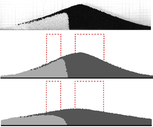
Figure 20 illustrates snapshots from the experiment, non-local and local modelling for the granular flow of Case II at t = 0.6 s. The interfaces obtained from the experimental measurement and non-local modelling were similar. The angle of the interface to the y-axes α was calculated without counting the particles in the vicinity of the free surface. This interface angle for the experiment was α = 5.3°, while α = 9.06° was calculated in the non-local modelling. There was a discrepancy in the interface angle between the non-local modelling and experimental measurements. This was proposed to arise from wall effects. The non-local modelling was conducted in two dimensionsr while the experiments for the flow occurred in a transparent Plexiglas channel in three dimensions. The flow in the experiment could be affected by the side-confined Plexiglas wall and the previous studies indicate that the wall can show a significant effect on the movement of the grains (Jop, Forterre & Pouliquen Reference Jop, Forterre and Pouliquen2005). The side wall can pose a drag force to the granular material so that the velocity of the grains close to the side wall could be affected. Without side-wall confinement, the interface in the experiment could be more curved, which would result in a larger angle that could be close to that obtained in the non-local modelling. The angle from the local modelling was much larger as α = 27.7°. In the local modelling, failure to capture the solid-like state plays a more important role in the interface angle in the comparison.

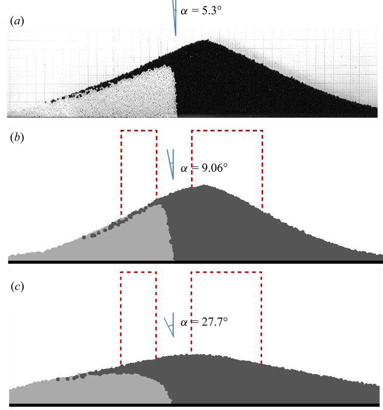
Figure 20. The interface in the collision of two adjacent collapsing columns for Case II at t = 0.60 s (The dashed line represents the original shape for the two granular columns): (a) the experimental measurement, (b) the non-local modelling and (c) the local modeling.