


1 Introduction
Flow-induced vibrations (FIV) of flexible or elastically mounted bodies with bluff cross-sections are omnipresent in nature (e.g. oscillations of trees in wind) and are also common in many civil, offshore and nuclear engineering applications (e.g. vibrations of mooring lines and cables exposed to ocean currents). These vibrations impact the fatigue life of the structures and often cause an amplification of the forces exerted on their supports. In the context of renewable energy production, they may also be used to harvest energy from wind or water streams. The fundamental mechanisms of FIV have been the object of a number of studies, as collected in Blevins (Reference Blevins1990), Naudascher & Rockwell (Reference Naudascher and Rockwell1994) and Païdoussis, Price & de Langre (Reference Païdoussis, Price and de Langre2010).
The present study concerns the FIV of an elastically mounted, rigid circular cylinder forced to rotate about its axis. Such system may provide insights for applications where the rotation could be used to reduce or enhance structural responses. From a fundamental perspective, it represents a paradigm of symmetry breaking in fluid–structure interaction. This work follows three previous studies where the body was allowed to move in a single direction, either normal to the current (Bourguet & Lo Jacono Reference Bourguet and Lo Jacono2014), aligned with the current (Bourguet & Lo Jacono Reference Bourguet and Lo Jacono2015) or at an arbitrary angle (Bourguet Reference Bourguet2019). The objective here is to extend the analysis to the case where the cylinder is allowed to move in the plane perpendicular to its axis, i.e. with two degrees of freedom. As explicated hereafter, the responses of the two-degree-of-freedom oscillator are expected to differ from their one-degree-of-freedom counterparts. This may be regarded as a step towards real physical systems, which are generally not constrained to a single direction of motion.
The impact of a forced rotation on the flow and fluid forcing has been well documented in the case of a rigidly mounted, circular cylinder placed in a cross-current (Díaz et al. Reference Díaz, Gavaldà, Kawall, Keffer and Giralt1983; Badr et al. Reference Badr, Coutanceau, Dennis and Ménard1990; Chew, Cheng & Luo Reference Chew, Cheng and Luo1995; Kang, Choi & Lee Reference Kang, Choi and Lee1999; Stojković, Breuer & Durst Reference Stojković, Breuer and Durst2002; Mittal & Kumar Reference Mittal and Kumar2003; Pralits, Brandt & Giannetti Reference Pralits, Brandt and Giannetti2010; Aljure et al. Reference Aljure, Rodríguez, Lehmkuhl, Pérez-Segarra and Oliva2015). The term rigidly mounted indicates that the body, subjected or not to a forced rotation, cannot translate. In the following, the rotation rate ( $\unicode[STIX]{x1D6FC}$) is defined as the ratio between the cylinder surface velocity and the oncoming flow velocity. The Reynolds number (
 $Re$) is based on the body diameter and on the oncoming flow velocity. The rotation breaks the symmetry of the physical system. Even at low values of
  $\unicode[STIX]{x1D6FC}$, this symmetry breaking induces an asymmetry in the strength of the alternating von Kármán vortices and the appearance of a time-averaged force normal to the current (Magnus effect). The rotation leads to a cancellation of the alternating vortex shedding and force fluctuations above
  $\unicode[STIX]{x1D6FC}\approx 2$, over a wide range of
  $Re$ (
 $\unicode[STIX]{x1D6FC}=1.8$ for
  $Re=100$). An unsteady flow regime characterized by low-frequency, large-amplitude fluctuations of fluid forces has been reported at higher
  $\unicode[STIX]{x1D6FC}$, typically around
  $\unicode[STIX]{x1D6FC}=5$ for
  $Re=100$. The rotation also alters the flow three-dimensional transition scenario (e.g. Pralits, Giannetti & Brandt Reference Pralits, Giannetti and Brandt2013; Radi et al. Reference Radi, Thompson, Rao, Hourigan and Sheridan2013; Rao et al. Reference Rao, Leontini, Thompson and Hourigan2013; Navrose, Meena & Mittal Reference Meena and Mittal2015).
On the other hand, the FIV of rigid bluff bodies have also been extensively investigated, in the absence of rotation. Vortex-induced vibrations (VIV) and motion-induced vibrations (MIV) are the two forms of FIV usually encountered for bluff bodies. A non-rotating, rigid circular cylinder has often served as a canonical problem to study VIV (Feng Reference Feng1968; Bearman Reference Bearman1984, Reference Bearman2011; Mittal & Tezduyar Reference Mittal and Tezduyar1992; Hover, Techet & Triantafyllou Reference Hover, Techet and Triantafyllou1998; Khalak & Williamson Reference Khalak and Williamson1999; Blackburn, Govardhan & Williamson Reference Blackburn, Govardhan and Williamson2000; Shiels, Leonard & Roshko Reference Shiels, Leonard and Roshko2001; Okajima, Kosugi & Nakamura Reference Okajima, Kosugi and Nakamura2002; Sarpkaya Reference Sarpkaya2004; Williamson & Govardhan Reference Williamson and Govardhan2004; Lucor, Foo & Karniadakis Reference Lucor, Foo and Karniadakis2005; Klamo, Leonard & Roshko Reference Klamo, Leonard and Roshko2006; Leontini et al. Reference Leontini, Stewart, Thompson and Hourigan2006; Dahl et al. Reference Dahl, Hover, Triantafyllou and Oakley2010; Cagney & Balabani Reference Cagney and Balabani2013; Konstantinidis Reference Konstantinidis2014; Gsell, Bourguet & Braza Reference Gsell, Bourguet and Braza2016; Navrose & Mittal Reference Mittal2016; Yao & Jaiman Reference Yao and Jaiman2017; Riches & Morton Reference Riches and Morton2018; Gurian, Currier & Modarres-Sadeghi Reference Gurian, Currier and Modarres-Sadeghi2019). These vibrations are driven by a mechanism of synchronization, referred to as lock-in, between body motion and flow unsteadiness associated with vortex shedding. In the above mentioned configuration, VIV generally develop over a well-defined range of the reduced velocity ( $U^{\star }$), i.e. inverse of the oscillator natural frequency non-dimensionalized by the inflow velocity and the body diameter. Within this range, vibration amplitudes exhibit bell-shaped evolutions as functions of
  $U^{\star }$. The maximum amplitudes are of the order of one body diameter in the direction normal to the current (cross-flow direction) and one or more orders of magnitude lower in the direction parallel to the current (in-line direction). MIV are another form of FIV which do not involve a coupling between the time scales of flow unsteadiness and body motion. MIV develop when the motion of the body tends to enhance the energy transfer from the flow to the structure (Blevins Reference Blevins1990). They can often be predicted through quasi-steady approaches, where each step of body oscillation is seen as a steady configuration by the flow (Parkinson & Smith Reference Parkinson and Smith1964). Due to the symmetry of the physical system, a non-rotating circular cylinder is not susceptible to MIV. However, as discussed in the next paragraph, such vibrations may arise due to the symmetry breaking caused by the rotation. Prior works concerning non-axisymmetric bodies have identified the main features of these self-excited vibrations, usually referred to as galloping responses (Den Hartog Reference Den Hartog1932; Mukhopadhyay & Dugundji Reference Mukhopadhyay and Dugundji1976; Nakamura & Tomonari Reference Nakamura and Tomonari1977; Tamura Reference Tamura1999; Hémon, Amandolese & Andrianne Reference Hémon, Amandolese and Andrianne2017). Contrary to VIV, their amplitudes tend to increase unboundedly with
  $U^{\star }$ and their frequencies are generally lower than VIV frequencies. Non-axisymmetric bodies often exhibit both VIV and MIV, and sometimes combinations of these vibration regimes (Bearman et al. Reference Bearman, Gartshore, Maull and Parkinson1987; Corless & Parkinson Reference Corless and Parkinson1988; Hémon & Santi Reference Hémon and Santi2002; Nemes et al. Reference Nemes, Zhao, Lo Jacono and Sheridan2012; Zhao et al. Reference Zhao, Leontini, Lo Jacono and Sheridan2014a; Mannini, Marra & Bartoli Reference Mannini, Marra and Bartoli2016; Seyed-Aghazadeh, Carlson & Modarres-Sadeghi Reference Seyed-Aghazadeh, Carlson and Modarres-Sadeghi2017; Zhao, Hourigan & Thompson Reference Zhao, Hourigan and Thompson2019). For non-rotating bodies, the possible differences appearing between one- and two-degree-of-freedom oscillator responses have been studied in previous works, for both MIV (Abdel-Rohman Reference Abdel-Rohman1992; Jones Reference Jones1992) and VIV (Jauvtis & Williamson Reference Jauvtis and Williamson2004; Cagney & Balabani Reference Cagney and Balabani2014; Gsell, Bourguet & Braza Reference Gsell, Bourguet and Braza2019). A typical example that illustrates the effect of adding a second degree of freedom to the oscillator occurs in the intermediate range of
  $U^{\star }$, for circular cylinder VIV (Gsell et al. Reference Gsell, Bourguet and Braza2019): no in-line vibrations develop in the one-degree-of-freedom case while such vibrations emerge if cross-flow motion is allowed; in addition, these in-line oscillations are accompanied by a major amplification of the cross-flow responses, compared to the one-degree-of-freedom case. Such alteration of the system behaviour, when a second degree of freedom is added, motivates the present work, where the impact of a forced rotation is explored for a two-degree-of-freedom oscillator.
The FIV of a rigid circular cylinder subjected to a forced rotation have been examined in recent studies. Most of these studies concern single-degree-of-freedom oscillators, where the cylinder is restrained to move either in the cross-flow direction (Bourguet & Lo Jacono Reference Bourguet and Lo Jacono2014; Zhao, Cheng & Lu Reference Zhao, Cheng and Lu2014b; Seyed-Aghazadeh & Modarres-Sadeghi Reference Seyed-Aghazadeh and Modarres-Sadeghi2015; Wong et al. Reference Wong, Zhao, Lo Jacono, Thompson and Sheridan2017) or in the in-line direction (Bourguet & Lo Jacono Reference Bourguet and Lo Jacono2015; Zhao et al. Reference Zhao, Lo Jacono, Sheridan, Hourigan and Thompson2018). Due to differences in the physical parameters of the experiments and numerical simulations (e.g. Reynolds number, structural damping, structure to displaced fluid mass ratio), the maximum amplitudes of vibration and the size of the vibration regions in the  $(\unicode[STIX]{x1D6FC},U^{\star })$ domain vary from one study to the other. However, general trends persist in all cases. In each direction, vibrations develop over a wide range of
  $\unicode[STIX]{x1D6FC}$, including beyond the critical value associated with the suppression of the von Kármán vortex street past a rigidly mounted cylinder. In the cross-flow direction, the response of the oscillator can be considerably amplified by the rotation. It, however, remains comparable to the VIV developing for
  $\unicode[STIX]{x1D6FC}=0$, including in the higher range of
  $\unicode[STIX]{x1D6FC}$: the lock-in condition is established, the vibration amplitude exhibits a bell-shaped evolution as a function of
  $U^{\star }$. For
  $Re=100$ and structural properties similar to those selected in the present work, a maximum amplitude of
  $1.9$ diameters was reported for
  $\unicode[STIX]{x1D6FC}=3.75$ (Bourguet & Lo Jacono Reference Bourguet and Lo Jacono2014). In the in-line direction, in contrast, two distinct regimes emerge in the
  $(\unicode[STIX]{x1D6FC},U^{\star })$ domain. VIV-like responses are still observed for low values of
  $\unicode[STIX]{x1D6FC}$. For larger values of
  $\unicode[STIX]{x1D6FC}$, typically
  $\unicode[STIX]{x1D6FC}>2.7$ for the same parameters as those selected in the present work, the vibrations resemble galloping responses, with amplitudes continuously increasing with
  $U^{\star }$. Body motion and flow unsteadiness remain synchronized for these galloping-like responses. More precisely, the spectral components of flow fluctuations occur at the vibration frequency and integer multiples of this frequency. The flow three-dimensional transition is delayed under cross-flow oscillation, i.e. the transition occurs at higher values of
  $\unicode[STIX]{x1D6FC}$ than for a rigidly mounted body. The opposite trend appears under in-line oscillation. In order to bridge the gap between the two above configurations and describe the passage from VIV- to galloping-like responses at high
  $\unicode[STIX]{x1D6FC}$, the orientation of the vibration plane was introduced as a new parameter of the problem in a previous work (Bourguet Reference Bourguet2019). In this work, it was shown that a quasi-steady modelling of fluid forcing predicts the emergence of galloping-like responses. The interaction with flow dynamics results, however, in clear deviations from the quasi-steady prediction. For example, the successive steps in the evolution of the vibration amplitude versus
  $U^{\star }$, associated with wake pattern switch, are not captured by the quasi-steady approach.
Only a few studies have addressed the case where the rotating cylinder is free to vibrate in both the in-line and cross-flow directions. Zhao et al. (Reference Zhao, Cheng and Lu2014b) focused on the alteration of the VIV for  $\unicode[STIX]{x1D6FC}\leqslant 1$. The symmetry breaking due to the rotation results in a switch from the typical figure-eight-shaped trajectories (e.g. Dahl et al. Reference Dahl, Hover, Triantafyllou and Oakley2010) to single-looped orbits. The main features of non-rotating body VIV persist in this range of
  $\unicode[STIX]{x1D6FC}$. Yet the differences occurring between the behaviours of the one- and two-degree-of-freedom oscillators are enhanced by the rotation. Stansby & Rainey (Reference Stansby and Rainey2001) studied the impact of higher
  $\unicode[STIX]{x1D6FC}$ values and showed that for
  $\unicode[STIX]{x1D6FC}\in [2,5]$, the two-degree-of-freedom oscillator can exhibit galloping-like, elliptical responses. Similar responses were observed by Yogeswaran & Mittal (Reference Yogeswaran, Mittal, Mittal and Biswas2011) for
  $\unicode[STIX]{x1D6FC}=4.5$. In this case, vortex formation is associated with high-frequency fluctuations of fluid forces, that are superimposed on the low-frequency oscillations related to body motion. By exploring specific regions of the
  $(\unicode[STIX]{x1D6FC},U^{\star })$ domain, previous works have shown that both VIV-like and galloping-like responses may be encountered for a two-degree-of-freedom oscillator. They have described some salient features of each form of response. A global vision of the system behaviour in this parameter space, including response regime transitions, is still missing. It appears that no systematic analysis of the flow dynamics and forcing has been reported for
  $\unicode[STIX]{x1D6FC}>1$. In addition, prior numerical simulations were based on two-dimensional flow assumption: the occurrence of three-dimensional transition and its effect on the responses is another aspect that needs to be clarified.
In the present work, the two-degree-of-freedom FIV of a rigid circular cylinder subjected to a forced rotation are investigated by means of two- and three-dimensional numerical simulations. The behaviour of the coupled flow–structure system is examined over a wide range of  $U^{\star }$ values, for
  $\unicode[STIX]{x1D6FC}\in [0,5.5]$. The Reynolds number is set to
  $100$ as in the above mentioned studies concerning single-degree-of-freedom oscillators (Bourguet & Lo Jacono Reference Bourguet and Lo Jacono2014, Reference Bourguet and Lo Jacono2015; Bourguet Reference Bourguet2019). For this value of
  $Re$, the selected range of
  $\unicode[STIX]{x1D6FC}$ includes the two unsteady flow regions identified for a rigidly mounted body (Stojković et al. Reference Stojković, Breuer and Durst2002), as well as the critical value associated with flow three-dimensional transition in this case (
 $\unicode[STIX]{x1D6FC}\approx 3.7$; Pralits et al. Reference Pralits, Giannetti and Brandt2013).
The paper is organized as follows. The physical model and the numerical method are presented in § 2. The rigidly mounted cylinder case is briefly addressed in § 3. The elastically mounted cylinder case is examined in § 4 through a joint analysis of the structural responses, flow physics and fluid forces. The main findings of this work are summarized in § 5.
2 Formulation and numerical method
The flow–structure configuration and its modelling are presented in § 2.1. The numerical method employed and its validation are described in § 2.2.
2.1 Physical system
A sketch of the physical system is presented in figure 1. The configuration is the same as in the previous works concerning rotating circular cylinders (Bourguet & Lo Jacono Reference Bourguet and Lo Jacono2014, Reference Bourguet and Lo Jacono2015; Bourguet Reference Bourguet2019), except that in the present study the elastically mounted, rigid body is free to move in both the in-line and cross-flow directions, instead of a single direction.

Figure 1. Sketch of the physical system.
The  $(x,y,z)$ frame is fixed. The axis of the cylinder is parallel to the
  $z$ axis. The body is placed in an incompressible cross-current which is aligned with the
  $x$ axis. The Reynolds number based on the oncoming flow velocity (
 $U$) and cylinder diameter (
 $D$),
$D$),  $Re=\unicode[STIX]{x1D70C}_{f}UD/\unicode[STIX]{x1D707}$, where
  $\unicode[STIX]{x1D70C}_{f}$ and
  $\unicode[STIX]{x1D707}$ denote the fluid density and viscosity, is set equal to
  $100$, as in the above mentioned works.
As suggested by prior studies and confirmed by the present results, the transition to three-dimensional flow occurs within the parameter space investigated. That is why the two-dimensional and three-dimensional Navier–Stokes equations are employed to predict the flow dynamics. In the three-dimensional case, the cylinder aspect ratio is set to  $L/D=24$, where
  $L$ is the cylinder length in the spanwise direction (
 $z$ axis). The increased aspect ratio compared to previous studies (where
  $L/D=10$) is justified by the emergence of longer spanwise wavelengths in some regions of the present parameter space, i.e. of the order of
  $4{-}5D$ versus
  $2D$ in prior works.
The cylinder can translate in the in-line direction ( $x$ axis) and in the cross-flow direction (
 $y$ axis). Its mass per unit length is denoted by
  $\unicode[STIX]{x1D70C}_{c}$. The structural stiffnesses and damping ratios are the same in the in-line and cross-flow directions; they are designated by
  $k$ and
  $\unicode[STIX]{x1D709}$, respectively. All the physical variables are non-dimensionalized by the cylinder diameter, the current velocity and the fluid density. The non-dimensional mass of the structure is defined as
  $m=\unicode[STIX]{x1D70C}_{c}/\unicode[STIX]{x1D70C}_{f}D^{2}$. The non-dimensional cylinder displacements, velocities and accelerations, in the in-line and cross-flow directions, are denoted by
  $\unicode[STIX]{x1D701}_{x}$,
  $\dot{\unicode[STIX]{x1D701}}_{x}$,
  $\ddot{\unicode[STIX]{x1D701}}_{x}$, and
  $\unicode[STIX]{x1D701}_{y}$,
  $\dot{\unicode[STIX]{x1D701}}_{y}$,
  $\ddot{\unicode[STIX]{x1D701}}_{y}$, respectively. The sectional in-line and cross-flow force coefficients are defined as
  $C_{xs}=2F_{xs}/\unicode[STIX]{x1D70C}_{f}DU^{2}$ and
  $C_{ys}=2F_{ys}/\unicode[STIX]{x1D70C}_{f}DU^{2}$, where
  $F_{xs}$ and
  $F_{ys}$ are the dimensional sectional fluid forces aligned with the
  $x$ and
  $y$ axes. The in-line and cross-flow force coefficients are the span-averaged values of the sectional force coefficients,
  $C_{x}=\langle C_{xs}\rangle$ and
  $C_{y}=\langle C_{ys}\rangle$, where
  $\langle \phantom{a}\rangle$ is the span-averaging operator; in the two-dimensional case,
  $C_{x}=C_{xs}$ and
  $C_{y}=C_{ys}$. The dynamics of the two-degree-of-freedom oscillator is governed by the following equations:
 $$\begin{eqnarray}\displaystyle & \displaystyle \ddot{\unicode[STIX]{x1D701}}_{x}+{\displaystyle \frac{4\unicode[STIX]{x03C0}\unicode[STIX]{x1D709}}{U^{\star }}}\dot{\unicode[STIX]{x1D701}}_{x}+\left({\displaystyle \frac{2\unicode[STIX]{x03C0}}{U^{\star }}}\right)^{2}\unicode[STIX]{x1D701}_{x}={\displaystyle \frac{C_{x}}{2m}}, & \displaystyle\end{eqnarray}$$
 $$\begin{eqnarray}\displaystyle & \displaystyle \ddot{\unicode[STIX]{x1D701}}_{y}+{\displaystyle \frac{4\unicode[STIX]{x03C0}\unicode[STIX]{x1D709}}{U^{\star }}}\dot{\unicode[STIX]{x1D701}}_{y}+\left({\displaystyle \frac{2\unicode[STIX]{x03C0}}{U^{\star }}}\right)^{2}\unicode[STIX]{x1D701}_{y}={\displaystyle \frac{C_{y}}{2m}}. & \displaystyle\end{eqnarray}$$
 $U^{\star }=1/f_{n}$, where
  $f_{n}$ is the non-dimensional natural frequency in vacuum,
  $f_{n}=D/2\unicode[STIX]{x03C0}U\sqrt{k/\unicode[STIX]{x1D70C}_{c}}$.
 The cylinder is subjected to a forced, counter-clockwise, steady rotation about its axis. The rotation is controlled by the rotation rate  $\unicode[STIX]{x1D6FC}=\unicode[STIX]{x1D6FA}D/2U$, where
  $\unicode[STIX]{x1D6FA}$ is the angular velocity of the cylinder.
The behaviour of the flow-structure system is explored in the  $(\unicode[STIX]{x1D6FC},U^{\star })$ parameter space, with
  $\unicode[STIX]{x1D6FC}\in [0,5.5]$ and
  $U^{\star }\in [1,25]$. As previously mentioned, the range of
  $\unicode[STIX]{x1D6FC}$ values under study encompasses the two unsteady flow regions reported at
  $Re=100$ for a rigidly mounted cylinder (Stojković et al. (Reference Stojković, Breuer and Durst2002), under two-dimensional flow assumption).
The structural damping is set equal to zero ( $\unicode[STIX]{x1D709}=0$) to allow maximum amplitude vibrations and
  $m$ is set equal to
  $10$, as in the above mentioned studies concerning single-degree-of-freedom oscillators. Additional simulations (not presented here) show that the principal features of the system behaviour persist when a low level of structural damping is added.
In addition to the elastically mounted body case, a series of two- and three-dimensional simulations is carried out for a rigidly mounted cylinder. A series of two-dimensional simulations where the cylinder is forced to translate at a constant velocity is also performed, to assess the validity of a quasi-steady modelling of fluid forcing.
2.2 Numerical method
The numerical method is the same as in previous studies concerning comparable flow–structure systems (e.g. Bourguet & Lo Jacono Reference Bourguet and Lo Jacono2014). It is briefly summarized here and some additional validation results are presented. The coupled flow–structure equations are solved by the parallelized code Nektar, which is based on the spectral/ $hp$ element method (Karniadakis & Sherwin Reference Karniadakis and Sherwin1999). A large rectangular computational domain is considered (
 $350D$ downstream and
  $250D$ in front, above, and below the cylinder) in order to avoid any spurious blockage effects due to domain size. A no-slip condition is applied on the cylinder surface. Flow periodicity conditions are employed on the side (spanwise) boundaries in the three-dimensional case.

Figure 2. Time-averaged (a) in-line and (b) cross-flow force coefficients as functions of the polynomial order, in the rigidly mounted cylinder case, for  $\unicode[STIX]{x1D6FC}=5$.

Figure 3. (a) Time-averaged in-line force coefficient, (b) time-averaged cross-flow force coefficient, (c) maximum amplitude of cross-flow vibration, (d) cross-flow frequency ratio, as functions of the polynomial order, in the elastically mounted cylinder case, for  $(\unicode[STIX]{x1D6FC},U^{\star })=(5.5,20)$.

Figure 4. Time series of the (a) in-line and (b) cross-flow force coefficients, over one vortex shedding period, in the rigidly mounted cylinder case, for  $\unicode[STIX]{x1D6FC}=5$. The present simulation results are compared to the time series reported by Stojković et al. (Reference Stojković, Breuer and Durst2002).
The parameter space explored in the present work includes higher values of  $\unicode[STIX]{x1D6FC}$ than those considered in the above mentioned studies. Two cases are selected in the higher range of
  $\unicode[STIX]{x1D6FC}$: (i)
  $\unicode[STIX]{x1D6FC}=5$ for the rigidly mounted body, which can be compared to prior simulation results from the literature and (ii)
  $(\unicode[STIX]{x1D6FC},U^{\star })=(5.5,20)$, where the elastically mounted cylinder exhibits very-large-amplitude oscillations. For each case, the evolutions of some physical quantities as functions of the spectral element polynomial order are plotted in figures 2 and 3 (two-dimensional simulations). The time-averaged force coefficients (
 $\overline{\phantom{a}}$ denotes time-averaged values) are represented in both cases. The maximum amplitude of cross-flow vibration (
 $\tilde{\phantom{a}}$ denotes the fluctuation about the time-averaged value), as well as the cross-flow frequency ratio (
 $f_{y}^{\star }=f_{y}/f_{n}$, where
  $f_{y}$ is the dominant frequency of cross-flow motion), are added in the elastically mounted body case. A polynomial order equal to
  $4$ is selected since an increase from order
  $4$ to
  $5$ has no significant impact on the results. It has also been verified, in these two cases, that dividing the non-dimensional time step by
  $2$ (i.e. from
  $0.0005$ to
  $0.00025$) has no influence. A comparison of the time evolutions of the force coefficients issued from the present study with the results reported by Stojković et al. (Reference Stojković, Breuer and Durst2002) in case (i) is presented in figure 4. In these plots and in the following,
  $t$ designates the non-dimensional time variable. The vortex shedding frequencies, time-averaged and peak-to-peak (subscript
  $_{pp}$) values of the force coefficients are compared in table 1. This comparison confirms the validity of the present numerical method. For the three-dimensional simulations,
  $128$ complex Fourier modes are employed in the spanwise direction. It has been verified that doubling the number of Fourier modes has only a negligible impact on the results. It has also been verified that the different flow structures encountered in the parameter space, including the subharmonic patterns, persist when the cylinder aspect ratio is varied (down to
  $5\unicode[STIX]{x03C0}$).
The simulations are initialized with the established periodic flow past a stationary cylinder at  $Re=100$. Then the forced rotation is started and the body is released. The analysis is based on time series of more than
  $40$ oscillation cycles, collected after convergence of the time-averaged and root mean square (r.m.s.) values of the fluid force coefficients and body displacements.
The entire parameter space is covered by two-dimensional simulations. The limits of the three-dimensional transition regions are identified via a first series of three-dimensional simulations. Three-dimensional simulation results are then collected in  $30$ cases,
  $9$ for the rigidly mounted body and
  $21$ for the elastically mounted body. The selected cases (i) cover the parameter space and (ii) provide a refined vision of the system behaviour at the edge of the large-amplitude vibration region for
  $\unicode[STIX]{x1D6FC}=5$.
Table 1. Vortex shedding frequency, time-averaged and peak-to-peak values of the in-line and cross force coefficients, in the rigidly mounted cylinder case, for  $\unicode[STIX]{x1D6FC}=5$.

3 Rigidly mounted cylinder
Before exploring the behaviour of the coupled flow–structure system, the case where the cylinder is rigidly mounted is briefly considered in this section. The objective here is to describe the impact of the imposed rotation on the flow and fluid forces, in the absence of vibration and for  $\unicode[STIX]{x1D6FC}\in [0,5.5]$.

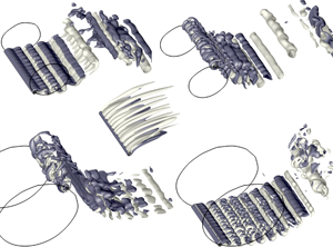
Figure 5. Instantaneous iso-surfaces of spanwise vorticity in the rigidly mounted body case: (a)  $\unicode[STIX]{x1D6FC}=1$, U1 regime, 2S pattern (
 $\unicode[STIX]{x1D714}_{z}=\pm 0.2$); (b)
  $\unicode[STIX]{x1D6FC}=3$, S1 regime,
  $D^{+}$ pattern (
 $\unicode[STIX]{x1D714}_{z}=\pm 0.04$); (c)
  $\unicode[STIX]{x1D6FC}=4$, S1 regime,
  $D^{-}$ pattern (
 $\unicode[STIX]{x1D714}_{z}=\pm 0.04$); (d)
  $\unicode[STIX]{x1D6FC}=4.5$, U2 regime (
 $\unicode[STIX]{x1D714}_{z}=\pm 0.06$); (e)
  $\unicode[STIX]{x1D6FC}=5$, U3 regime (
 $\unicode[STIX]{x1D714}_{z}=\pm 0.03$); (f)
  $\unicode[STIX]{x1D6FC}=5.5$, S2 regime,
  $D^{+}$ pattern (
 $\unicode[STIX]{x1D714}_{z}=\pm 0.004$). Positive/negative vorticity values are plotted in yellow/blue. Part of the computational domain is shown.

Figure 6. Flow regimes as functions of the rotation rate, in the rigidly mounted cylinder case. The different regimes are delimited by plain black lines and their names are indicated in black. Oblique blue stripes denote the region where the flow undergoes three-dimensional transition. The unsteady/steady flow regimes are indicated in grey/white. The region where the flow is found to be unsteady via three-dimensional simulations, whereas it remains steady under two-dimensional flow assumption (U2 regime), is denoted by a grey area with horizontal white stripes. The evolution of the dominant frequency of the cross-flow force coefficient as a function of the rotation rate is plotted in each unsteady flow region (three-dimensional simulation results in the three-dimensional flow region). Some typical wake patterns are indicated in brackets in green. The limit between the  $D^{+}$ and
  $D^{-}$ patterns (S1 regime) is denoted by a green dashed line.
An overview of the flow for selected values of  $\unicode[STIX]{x1D6FC}$ is presented in figure 5, by means of instantaneous iso-surfaces of spanwise vorticity (
 $z$ component). These visualizations confirm that a variety of regimes are encountered over the range of
  $\unicode[STIX]{x1D6FC}$ investigated: steady and unsteady, two- and three-dimensional, with more or less regular spanwise structures. A map of the different regimes is proposed in figure 6. The unsteady/steady flow regimes are indicated in grey/white. In a range of
  $\unicode[STIX]{x1D6FC}$ around
  $4.5$, the flow is found to be unsteady via three-dimensional simulations, whereas it remains steady under two-dimensional flow assumption. This region is denoted by a grey area with horizontal white stripes. The dominant frequency of the cross-flow force coefficient (
 $f_{C_{y}}$) is plotted in each unsteady flow regime. The region where the flow undergoes three-dimensional transition is indicated by oblique blue stripes. In the three-dimensional flow region, the values of
  $f_{C_{y}}$ are issued from three-dimensional simulations.
For  $\unicode[STIX]{x1D6FC}<1.8$, the flow is two-dimensional, unsteady and periodic. It is characterized by the formation of two counter-rotating, spanwise vortices per period (figure 5a). The rotation induces an asymmetry in the strength of the positive and negative vortices but flow structure remains comparable to the 2S pattern observed for
  $\unicode[STIX]{x1D6FC}=0$ (Williamson & Roshko Reference Williamson and Roshko1988). This asymmetry causes a switch in force frequency ratio, from
  $f_{C_{x}}=2f_{C_{y}}$ to
  $f_{C_{x}}=f_{C_{y}}$, where
  $f_{C_{x}}$ is the dominant frequency of the in-line force coefficient. Wake frequency (equal to
  $f_{C_{y}}$) only slightly deviates from the Strouhal frequency (i.e. vortex shedding frequency for
  $\unicode[STIX]{x1D6FC}=0$,
  $f_{St}=0.164$). This first unsteady regime is referred to as Unsteady 1 (U1) in the following. When
  $\unicode[STIX]{x1D6FC}$ is increased beyond
  $1.8$ and up to
  $4.15$ approximately, the flow is steady. This first steady regime is referred to as Steady 1 (S1). The flow undergoes three-dimensional transition for
  $\unicode[STIX]{x1D6FC}\approx 3.7$, as reported in prior studies (Pralits et al. Reference Pralits, Giannetti and Brandt2013; Rao et al. Reference Rao, Leontini, Thompson and Hourigan2013). The wake is composed of two layers of vorticity of opposite signs and deflected upwards (figure 5b,c). At a rotation rate comparable to the critical value for three-dimensional transition (
 $\unicode[STIX]{x1D6FC}\approx 3.7$), a switch of the two layers of vorticity can be noted in the wake. This switch is accompanied by a change in the sign of the in-line force (i.e. drag), as shown hereafter. The two steady wake patterns were called
  $D^{+}$ and
  $D^{-}$ in a previous work (Bourguet & Lo Jacono Reference Bourguet and Lo Jacono2014), in reference to the positive or negative value of the drag. In the S1 regime, the three-dimensional flow exhibits a regular spanwise alignment of elongated streamwise tongues of vorticity. A typical wavelength of
  $1.6$ body diameters appears for
  $\unicode[STIX]{x1D6FC}=4$. For comparison, in the absence of rotation, the three-dimensional transition occurs at
  $Re\approx 190$ with a critical wavelength close to
  $4$ diameters (Williamson Reference Williamson1996). A second region of unsteady flow emerges when the rotation rate is further increased. From
  $\unicode[STIX]{x1D6FC}=4.15$ to
  $\unicode[STIX]{x1D6FC}=4.8$ approximately, the flow is globally comparable to that observed in the three-dimensional part of the S1 regime. However, it is now unsteady and the spanwise alignment of the streamwise tongues of vorticity is more erratic (figure 5d). The dominant spanwise wavelength slightly increases, e.g. close to
  $2$ body diameters for
  $\unicode[STIX]{x1D6FC}=4.5$. The flow time evolution is less regular than in the U1 regime. The typical frequency of flow unsteadiness, quantified via
  $f_{C_{y}}$, is close to
  $0.04$ and thus substantially lower than in the first unsteady regime. An important aspect is that the flow remains steady in this range of
  $\unicode[STIX]{x1D6FC}$ under two-dimensional flow assumption, as previously reported by Stojković et al. (Reference Stojković, Breuer and Durst2002). Following the above nomenclature, this regime is called Unsteady 2 (U2). Another unsteady regime appears from
  $\unicode[STIX]{x1D6FC}=4.8$ to
  $\unicode[STIX]{x1D6FC}=5.15$, approximately. Contrary to the U2 regime, it also exists under two-dimensional flow assumption (e.g. Stojković et al. Reference Stojković, Breuer and Durst2002), even though the flow is actually three-dimensional in this regime. The flow is close to periodic. It is characterized by the shedding of a single, large-scale, (positive) spanwise vortex per cycle, at low frequency compared to the U1 regime (figure 5e). The shedding frequency, close to
  $0.02$, tends to decrease with
  $\unicode[STIX]{x1D6FC}$ in this regime. The well-defined spanwise undulation presents a typical wavelength close to
  $5$ diameters. This third unsteady regime is referred to as Unsteady 3 (U3). Beyond
  $\unicode[STIX]{x1D6FC}=5.15$ and up to
  $\unicode[STIX]{x1D6FC}=5.5$, the flow is found to be steady and two-dimensional (figure 5f). Wake structure globally resembles the
  $D^{+}$ pattern observed in the first part of the S1 regime. This second steady regime is referred to as Steady 2 (S2). The names of the different flow regimes, as well as those of the typical wake patterns are indicated in the map in figure 6.

Figure 7. (a,b) Time-averaged value of the force coefficient and (c,d) r.m.s. value of the force coefficient fluctuation, in the (a,c) in-line and (b,d) cross-flow directions, as functions of the rotation rate, in the rigidly mounted cylinder case. The colour code employed to designate the unsteady and steady flow regimes is the same as in figure 6. In the region of three-dimensional flow (oblique blue stripes in figure 6), both two- and three-dimensional simulation results are presented.
To further describe these regimes, the time-averaged values of the force coefficients and the r.m.s. values of their fluctuations are presented in figure 7. In the three-dimensional flow region (from  $\unicode[STIX]{x1D6FC}=3.7$ to
  $\unicode[STIX]{x1D6FC}=5.15$ approximately), both two- and three-dimensional simulation results are reported in order to quantify the influence of the three-dimensional transition. The mean in-line force decreases as a function of the rotation rate, until
  $\unicode[STIX]{x1D6FC}\approx 4$, where it starts increasing with
  $\unicode[STIX]{x1D6FC}$. It becomes slightly negative over a short interval around
  $\unicode[STIX]{x1D6FC}=4$. Its evolution appears relatively smooth through the successive flow regimes. A substantial increase can, however, be noted between the U2 and U3 regimes. The mean cross-flow force monotonically decreases over the range of
  $\unicode[STIX]{x1D6FC}$ investigated, with no noticeable impact of the passage from one flow regime to the other. The r.m.s. values vanish when the flow is steady. A major amplification of the force coefficient fluctuations can be noted in the U3 regime, compared to the U1 regime. In contrast, only low-magnitude fluctuations are observed in the U2 regime. It should be mentioned that these plots quantify the fluctuations of the span-averaged forces. Low r.m.s. values of
  $\tilde{C}_{x}$ and
  $\tilde{C}_{y}$ do not necessarily imply that the temporal fluctuations of the sectional forces (or any local flow quantity) are small. In the U2 regime, force fluctuations only occur in the three-dimensional simulation results since the flow is found to be steady under two-dimensional flow assumption. Otherwise, only slight differences can be noted between two- and three-dimensional simulation results.

Figure 8. Selected times series of the (top) in-line force coefficient ( $C_{x}$) and sectional force coefficient at midspan (
 $C_{xs}$ at
  $z=12$) and (bottom) fluctuation of the sectional in-line force coefficient about its span-averaged value, in the rigidly mounted cylinder case, for (a)
  $\unicode[STIX]{x1D6FC}=4$ (S1 regime), (b)
  $\unicode[STIX]{x1D6FC}=4.5$ (U2 regime) and (c)
  $\unicode[STIX]{x1D6FC}=5$ (U3 regime). In the bottom plot of each panel, a dashed-dotted line indicates the midspan point where
  $C_{xs}$ (represented in the top plot) is sampled.
Some additional observations concerning the three-dimensional flows are presented on the basis of selected time series of the in-line force, plotted in figure 8. In this figure, time series of  $C_{x}$,
  $C_{xs}$ at midspan point (
 $z=12$), and the fluctuation of
  $C_{xs}$ about
  $C_{x}$, are plotted for a selected value of
  $\unicode[STIX]{x1D6FC}$ in each regime of the three-dimensional flow region, i.e. S1, U2 and U3 regimes. It is recalled that
  $C_{xs}$ designates the sectional force coefficient while
  $C_{x}$ is the span-averaged value of
  $C_{xs}$. Comparison of
  $C_{x}$ and
  $C_{xs}$ at an arbitrary point (here midspan point) illustrates the variability of the local force magnitude and its possibly large temporal fluctuations, even if the span-averaged coefficient exhibits a low r.m.s. value (figure 8b). This comparison also reveals some features of flow structure: the periodic difference noted between
  $C_{x}$ and
  $C_{xs}$ at midspan point in figure 8(c) betrays the existence of a subharmonic component in the three-dimensional flow pattern. The spatio-temporal evolution of the force fluctuation provides a complementary vision of the flow (bottom plots in figure 8). It confirms the emergence of different spanwise wavelengths depending on the value of
  $\unicode[STIX]{x1D6FC}$ and the more or less regular nature of the spanwise structure. As previously mentioned, flow structure in the U2 regime appears as an unsteady and slightly disordered version of the S1 regime structure. The spatio-temporal plot for
  $\unicode[STIX]{x1D6FC}=5$ (figure 8c) emphasizes the subharmonic component developing in the U3 regime, at half the spanwise vortex shedding frequency.
To summarize, a variety of flow regimes are encountered in the rigidly mounted body case over the range of  $\unicode[STIX]{x1D6FC}$ considered in this work. Unsteady flow regimes develop in two distinct regions: in the lower range of
  $\unicode[STIX]{x1D6FC}$ (U1 regime) where the flow remains two-dimensional and globally close to that observed for
  $\unicode[STIX]{x1D6FC}=0$ and in the higher range of
  $\unicode[STIX]{x1D6FC}$, where two successive three-dimensional flow regimes emerge (U2 and U3 regimes). These two regimes are both characterized by lower frequencies than the U1 regime. They exhibit contrasted spatio-temporal properties, associated with different magnitudes of fluid forcing. In particular, a major amplification of fluid force fluctuations occurs in the U3 regime, which is dominated by the shedding of a single, large-scale, spanwise vortex. Beyond a brief description of the rigidly mounted cylinder case, the preliminary observations reported here will serve as reference to quantify the alteration of flow physics once the body is subjected to flow-induced vibrations.
4 Elastically mounted cylinder
The behaviour of the coupled flow–structure system is investigated for  $\unicode[STIX]{x1D6FC}\in [0,5.5]$ and
  $U^{\star }\in [1,25]$. The structural responses are described in § 4.1. Flow physics is analysed in § 4.2 and fluid forces are examined in § 4.3.
4.1 Structural responses
An overview of the flow-induced vibrations of the cylinder is presented in figure 9. In figure 9(a,b), the maximum in-line and cross-flow oscillation amplitudes of the body about its time-averaged position are plotted in the  $(\unicode[STIX]{x1D6FC},U^{\star })$ domain. The plots are based on two-dimensional simulation results. These results provide a global vision of the response trends, even in the higher range of
  $\unicode[STIX]{x1D6FC}$ values where the flow undergoes three-dimensional transition (§ 4.2). The three-dimensional simulation results presented in the following confirm the trends described under two-dimensional flow assumption.

Figure 9. (a,b) Maximum amplitude of vibration in the (a) in-line and (b) cross-flow directions and (c) vibration region, as functions of the rotation rate and reduced velocity. In (c), the area where the cylinder exhibits oscillations of any amplitudes is denoted by a grey background and delimited by plain black lines; the regions where vibrations are predicted by three-dimensional simulations but not under two-dimensional flow assumption are indicated by vertical white stripes superimposed over the grey background; the large-amplitude vibration region (i.e.  $(\tilde{\unicode[STIX]{x1D701}}_{y})_{\text{max}}>0.03$) is indicated by horizontal, dark grey stripes; black dotted lines represent iso-lines of the maximum amplitude of cross-flow vibration; oblique red stripes denote the area where subharmonic components appear in the responses; the value of the cross-flow force–displacement phase difference, within the large-amplitude vibration region, is specified in orange and an orange dotted line denotes the location of the phase difference jump (no jump occurs in the galloping-like response region); the limits of the large-amplitude vibration regions identified for the cross-flow oscillator (Bourguet & Lo Jacono Reference Bourguet and Lo Jacono2014) and the in-line oscillator (Bourguet & Lo Jacono Reference Bourguet and Lo Jacono2015) are indicated by blue dashed lines and green dashed-dotted lines, respectively.
Based on the evolutions of the vibration amplitudes as functions of  $U^{\star }$, two distinct forms of responses can be identified. The significant vibrations that occur until
  $\unicode[STIX]{x1D6FC}=2$ approximately, appear over a well-defined range of
  $U^{\star }$, where they exhibit bell-shaped evolutions. In this region of the parameter space, the rotation alters the magnitude of the response curves but they remain essentially comparable to those observed for the typical VIV of a non-rotating circular cylinder. After a transition region around
  $\unicode[STIX]{x1D6FC}=2$, and up to the largest rotation rate under study (
 $\unicode[STIX]{x1D6FC}=5.5$), the vibrations present galloping-like evolutions, i.e. their amplitudes tend to grow unboundedly with
  $U^{\star }$. The growth rate of the galloping-like responses increases regularly with
  $\unicode[STIX]{x1D6FC}$. Amplitudes larger than
  $20$ body diameters are reached in the present parameter space. It can be noted that the transition from VIV-like to galloping-like responses occurs simultaneously in the in-line and cross-flow directions. These results corroborate prior experimental and numerical observations (e.g. Stansby & Rainey Reference Stansby and Rainey2001; Bourguet & Lo Jacono Reference Bourguet and Lo Jacono2014; Wong et al. Reference Wong, Zhao, Lo Jacono, Thompson and Sheridan2017) concerning the appearance of FIV in ranges of
  $\unicode[STIX]{x1D6FC}$ where the rotation leads to a cancellation of flow unsteadiness in the rigidly mounted body case (here between
  $\unicode[STIX]{x1D6FC}=1.8$ and
  $\unicode[STIX]{x1D6FC}=4.15$ and beyond
  $\unicode[STIX]{x1D6FC}=5.15$). They also confirm that the two-degree-of-freedom oscillator may exhibit both VIV-like and galloping-like responses, depending on the rotation rate value. This was previously suggested by separate studies focusing either on low values of
  $\unicode[STIX]{x1D6FC}$ (VIV-like responses; Zhao et al. (Reference Zhao, Cheng and Lu2014b)) or on high values of
  $\unicode[STIX]{x1D6FC}$ (galloping-like responses; Stansby & Rainey (Reference Stansby and Rainey2001), Yogeswaran & Mittal (Reference Yogeswaran, Mittal, Mittal and Biswas2011)).
Another visualization of the structural responses is proposed in figure 9(c) which represents a map of the vibration region in the  $(\unicode[STIX]{x1D6FC},U^{\star })$ domain. The map is based on a combination of two- and three-dimensional simulation results. In this map, the area of the parameter space where the cylinder exhibits oscillations of any amplitudes is denoted by a grey background. In two regions, located around
  $\unicode[STIX]{x1D6FC}=4.5$ and identified by vertical white stripes superimposed over the grey background, vibrations are predicted by three-dimensional simulations but not under two-dimensional flow assumption. The cylinder exhibits some oscillations for any values of
  $U^{\star }$ in the ranges of
  $\unicode[STIX]{x1D6FC}$ values where the flow is unsteady in the rigidly mounted body case (§ 3). It is recalled that, in the rigidly mounted body case, the U2 regime is not captured under two-dimensional flow assumption. The difference noted between the two- and three-dimensional simulation results for
  $U^{\star }<3.5$ around
  $\unicode[STIX]{x1D6FC}=4.5$ (vertically striped area) is thus expected. The region where the maximum amplitude of cross-flow oscillation is larger than
  $0.03$ is indicated by horizontal, dark grey stripes. This region is referred to as large-amplitude vibration region in the following. The areas of this region characterized by VIV-like and galloping-like responses, roughly below and above
  $\unicode[STIX]{x1D6FC}=2$, are specified in the map. For comparison purpose, the limits of the large-amplitude vibration regions previously identified for the cross-flow oscillator (Bourguet & Lo Jacono Reference Bourguet and Lo Jacono2014) and the in-line oscillator (Bourguet & Lo Jacono Reference Bourguet and Lo Jacono2015) are also plotted. It should be noted that the definitions of the large-amplitude vibration regions in these prior studies were slightly different and that the range of
  $\unicode[STIX]{x1D6FC}$ investigated was limited to
  $\unicode[STIX]{x1D6FC}=3.5$ and
  $\unicode[STIX]{x1D6FC}=4$, for the in-line and cross-flow oscillators, respectively. However, the comparison reveals some major deviations between the responses of the one- and two-degree-of-freedom oscillators. Such deviations have been documented for non-rotating cylinder VIV (e.g. Gsell et al. Reference Gsell, Bourguet and Braza2019). The motion of the cylinder in one direction may dramatically alter the orientation and magnitude of the relative velocity seen by the body, and thus impact the forcing (and response) in the perpendicular direction. In the present case, galloping-like responses appear at much lower
  $\unicode[STIX]{x1D6FC}$ for the two-degree-of-freedom oscillator than for the in-line oscillator, which exhibits such responses only beyond a rotation rate close to
  $2.7$. In the first region located in the lower range of
  $\unicode[STIX]{x1D6FC}$ values, the in-line oscillator is subjected to VIV-like responses. The contrast is even more pronounced with the behaviour of the cross-flow oscillator. Up to
  $\unicode[STIX]{x1D6FC}\approx 4$, within the area indicated in the map, it does not exhibit galloping-like oscillations but only VIV-like responses. The in-line oscillator remains steady from
  $\unicode[STIX]{x1D6FC}\approx 2$ to
  $\unicode[STIX]{x1D6FC}\approx 2.7$, which is another remarkable difference. The other elements plotted in the map will be discussed later in the paper.
A more quantitative description of the structural responses is presented in the following. In most cases, the vibrations are periodic and dominated by a single frequency with some limited higher harmonic contributions, i.e. close to sinusoidal. Some cases where other spectral components emerge will be examined at the end of this section. The term vibration frequency refers to the dominant vibration frequency, which is denoted by  $f_{x}$ in the in-line direction and
  $f_{y}$ in the cross-flow direction. The deviation between the vibration frequency and the natural frequency of the oscillator (
 $f_{n}$) is measured, in each direction, via the frequency ratio,
  $f_{x}^{\star }=f_{x}/f_{n}$ and
  $f_{y}^{\star }=f_{y}/f_{n}$.

Figure 10. (a–d) Maximum amplitude of vibration in the (a,b) in-line and (c,d) cross-flow directions, and (e,f) cross-flow frequency ratio, as functions of the reduced velocity, for (a,c,e)  $\unicode[STIX]{x1D6FC}\leqslant 2$ and (b,d,f)
  $\unicode[STIX]{x1D6FC}\geqslant 2$. In (e,f) black dashed, dotted and dashed-dotted lines indicate typical frequencies (normalized by the oscillator natural frequency) of flow unsteadiness in the rigidly mounted cylinder case, for
  $\unicode[STIX]{x1D6FC}=0$ (U1 regime),
  $\unicode[STIX]{x1D6FC}=4.5$ (U2 regime) and
  $\unicode[STIX]{x1D6FC}=5$ (U3 regime), respectively. The three-dimensional simulation results are denoted by circled blue symbols. The results obtained in the one-degree-of-freedom cases (Bourguet & Lo Jacono Reference Bourguet and Lo Jacono2014, Reference Bourguet and Lo Jacono2015) for (a,c,e)
  $\unicode[STIX]{x1D6FC}=1$ and (b,d,f)
  $\unicode[STIX]{x1D6FC}=3$ are also reported (plain/dashed-dotted red lines for the in-line/cross-flow oscillators).
The maximum amplitudes of the in-line and cross-flow responses, as well as the cross-flow frequency ratio, are plotted in figure 10, as functions of  $U^{\star }$, for each value of
  $\unicode[STIX]{x1D6FC}$. For more clarity due to scale differences, the data collected for
  $\unicode[STIX]{x1D6FC}\leqslant 2$ and
  $\unicode[STIX]{x1D6FC}\geqslant 2$ are presented separately in figures 10(a,c,e) and 10(b,d,f), respectively; this corresponds to the separation between the VIV-like and galloping-like responses. The entire parameter space is covered by two-dimensional simulations and selected three-dimensional simulation results are also reported for comparison purpose (circled blue symbols).
In the in-line direction, the rotation induces a regular amplification of the bell-shaped responses. It can be noted that a slow rotation already results in a major enhancement of the maximum oscillation amplitude: close to  $0.3$ diameters for
  $\unicode[STIX]{x1D6FC}=0.5$ versus
  $0.02$ diameters for
  $\unicode[STIX]{x1D6FC}=0$. An increasing trend is also observed in the cross-flow direction except in the lower range of
  $\unicode[STIX]{x1D6FC}$ where the rotation causes a slight reduction of the response amplitude. For a given
  $(\unicode[STIX]{x1D6FC},U^{\star })$ point in the VIV-like response region, the cross-flow oscillation amplitude remains generally larger than the in-line amplitude, as in the absence of rotation. In the upper part of this region, the peak amplitudes in both directions are approximately twice larger, i.e. around
  $1$ body diameter, than the peak amplitude of cross-flow VIV for
  $\unicode[STIX]{x1D6FC}=0$. Beyond the transition region illustrated by the irregular response curves obtained for
  $\unicode[STIX]{x1D6FC}=2$, the galloping-like oscillation amplitudes continuously increase with
  $\unicode[STIX]{x1D6FC}$. In each point of the galloping-like response region beyond
  $U^{\star }\approx 7$, the oscillation amplitude is found to be larger in the in-line direction than in the cross-flow direction, i.e. the opposite trend compared to the VIV-like response region. In the lower part of the galloping-like response region (up to
  $\unicode[STIX]{x1D6FC}=4$), successive steps can be identified in the response curves. Comparable steps have been connected to wake pattern switch in a previous work concerning a single-degree-of-freedom oscillator (Bourguet Reference Bourguet2019). They tend to vanish at higher rotation rates.
Once the system symmetry is broken by the rotation, the in-line and cross-flow vibration frequencies are generally the same, whereas  $f_{x}=2f_{y}$ for
  $\unicode[STIX]{x1D6FC}=0$. Such frequency switch, previously noted for non-axisymmetric cross-sections (Naudascher Reference Naudascher1987), relates to the alteration of the anti-symmetric nature of the wake and to the associated modification of the in-line forcing frequency. To avoid redundant information, only the cross-flow frequency ratio is presented in figure 10(e,f). Out of the large-amplitude vibration region, the response frequency remains close to the frequency of flow unsteadiness in the rigidly mounted body case. The typical frequencies identified in the U1, U2 and U3 regimes (§ 3) are indicated by discontinuous black lines. Within the large-amplitude vibration region, the response frequency deviates both from these typical frequencies and from the oscillator natural frequency (
 $f_{y}^{\star }\neq 1$ in general). It can be noted that the vibration frequency crosses the natural frequency in the VIV-like response region while the galloping-like responses always occur at a lower frequency. This observation is connected to force–displacement phasing, as discussed in § 4.3. The vibration frequency tends to globally decrease as
  $\unicode[STIX]{x1D6FC}$ is increased, which confirms the trend predicted by the potential flow analysis proposed by Stansby & Rainey (Reference Stansby and Rainey2001). It reaches very low values, close to
  $f_{n}/4$ for
  $\unicode[STIX]{x1D6FC}=5.5$.
The three-dimensional simulation results reported in figure 10 show that the flow three-dimensional transition has only a limited effect on the oscillator responses. An element can, however, be noted: some deviations between the two- and three-dimensional simulation results are observed down to  $\unicode[STIX]{x1D6FC}=2$. This indicates that the transition occurs at a much lower value of
  $\unicode[STIX]{x1D6FC}$ than in the rigidly mounted body case (where the critical value is close to
  $3.7$).
The shapes, magnitudes and frequencies of the two-degree-of-freedom oscillator responses differ from those observed at the same  $\unicode[STIX]{x1D6FC}$, in the single-degree-of-freedom cases. This is visualized in figure 10, where the maximum amplitudes obtained for the in-line and cross-flow oscillators, and the cross-flow oscillator frequency ratios are represented by red lines, for
  $\unicode[STIX]{x1D6FC}=1$ and
  $\unicode[STIX]{x1D6FC}=3$. The addition of a second degree of freedom is accompanied by a pronounced amplification of the in-line oscillations, in both the VIV-like and galloping-like response regions. In the cross-flow direction, the switch from VIV-like to galloping-like responses for
  $\unicode[STIX]{x1D6FC}=3$ is associated with a major reduction of the vibration frequency.

Figure 11. Phase difference between the dominant components of the in-line and cross-flow responses as a function of the reduced velocity, within the large-amplitude vibration region identified in figure 9(c), for (a)  $\unicode[STIX]{x1D6FC}\leqslant 2$ and (b)
  $\unicode[STIX]{x1D6FC}\geqslant 2$. The ratio between the frequencies of the dominant components of the in-line and cross-flow responses is indicated in the plots. The three-dimensional simulation results are denoted by circled blue symbols.
The synchronization between the in-line and cross-flow responses is monitored via the phase difference  $\unicode[STIX]{x1D6F7}_{xy}=\unicode[STIX]{x1D719}_{x}-n\unicode[STIX]{x1D719}_{y}$, where
  $\unicode[STIX]{x1D719}_{x}$ and
  $\unicode[STIX]{x1D719}_{y}$ are the phases of the dominant spectral components of the in-line and cross-flow responses, and
  $n$ is the ratio of their frequencies, i.e.
  $n=2$ for
  $\unicode[STIX]{x1D6FC}=0$ and
  $n=1$ otherwise (e.g. Bourguet, Karniadakis & Triantafyllou Reference Bourguet, Karniadakis and Triantafyllou2013). In the following, the phase difference is wrapped between
  $0^{\circ }$ and
  $360^{\circ }$. For
  $n=2$, the cylinder describes figure-eight trajectories and moves upstream when reaching cross-flow oscillation maxima for
  $\unicode[STIX]{x1D6F7}_{xy}\in ]\!0^{\circ },180^{\circ }\![$ and downstream for
$\unicode[STIX]{x1D6F7}_{xy}\in ]\!0^{\circ },180^{\circ }\ $\unicode[STIX]{x1D6F7}_{xy}\in ]\!180^{\circ },360^{\circ }\![$. These two types of trajectories were referred to as counter-clockwise and clockwise, figure-eight orbits in previous works (Dahl et al. Reference Dahl, Hover, Triantafyllou and Oakley2010). The cases
$\unicode[STIX]{x1D6F7}_{xy}\in ]\!180^{\circ },360^{\circ }\ $\unicode[STIX]{x1D6F7}_{xy}=0^{\circ }$ and
  $\unicode[STIX]{x1D6F7}_{xy}=180^{\circ }$ correspond to crescent-shaped trajectories. For
  $n=1$, the cylinder describes elliptical trajectories in the counter-clockwise direction for
  $\unicode[STIX]{x1D6F7}_{xy}\in ]\!0^{\circ },180^{\circ }\![$ and in the clockwise direction for
$\unicode[STIX]{x1D6F7}_{xy}\in ]\!0^{\circ },180^{\circ }\ $\unicode[STIX]{x1D6F7}_{xy}\in ]\!180^{\circ },360^{\circ }\![$. For
$\unicode[STIX]{x1D6F7}_{xy}\in ]\!180^{\circ },360^{\circ }\ $\unicode[STIX]{x1D6F7}_{xy}=0^{\circ }$ and
  $\unicode[STIX]{x1D6F7}_{xy}=180^{\circ }$, the trajectories are linear. The evolution of the phase difference within the large-amplitude vibration region identified in figure 9(c) is plotted in figure 11. In the absence of rotation, the cylinder exhibits counter-clockwise, figure-eight orbits. Once the body rotates, the phase difference of the VIV-like responses varies between
  $270^{\circ }$ and
  $180^{\circ }$ approximately, i.e. between clockwise elliptical orbits and linear trajectories. In contrast, a single type of trajectories appears in the galloping-like response region: the cylinder describes clockwise elliptical orbits, since
  $\unicode[STIX]{x1D6F7}_{xy}\approx 270^{\circ }$ in all cases. It is recalled that the forced rotation applied to the cylinder is oriented in the opposite direction (counter-clockwise). The elliptical orbits are referred to as counter-rotating. An elliptical trajectory, typical of the galloping-like response region, is plotted in figure 12(a). Some slight variations about this canonical shape may be encountered, in particular due to the emergence of subharmonic components as discussed in the following. However, the global form of the trajectory remains the same. These observations regarding response phasing are confirmed by the three-dimensional simulation results (circled blue symbols in figure 11). In the plot presented in figure 12(a), it can be noted that the orbits issued from the two- and three-dimensional simulations are almost identical, even if the flow is three-dimensional in the selected case (§ 4.2). Similar counter-rotating orbits were reported in prior studies concerning galloping-like oscillations (Stansby & Rainey Reference Stansby and Rainey2001; Yogeswaran & Mittal Reference Yogeswaran, Mittal, Mittal and Biswas2011). A quasi-steady analysis may suggest such orientation of the elliptical trajectories, as briefly discussed in an Appendix.

Figure 12. Typical trajectories of the rotating cylinder in the large-amplitude vibration region: (a)  $(\unicode[STIX]{x1D6FC},U^{\star })=(4,17)$, (b)
  $(\unicode[STIX]{x1D6FC},U^{\star })=(4,6)$ (period doubling), (c)
  $(\unicode[STIX]{x1D6FC},U^{\star })=(5,6)$ (period quadrupling). The black lines represent two-dimensional simulation results while the grey lines (in a,b) denote three-dimensional simulation results. Three dominant frequency cycles are plotted in each case.
As previously mentioned, the structural responses are close to sinusoidal in most cases. Within the large-amplitude response region, the dominant vibration components are often accompanied by higher harmonic contributions, the most significant being those occurring at  $2f_{x}$ and
  $2f_{y}$ in the galloping-like response region. Their magnitudes remain limited, typically lower than
  $10\,\%$ of the dominant component amplitudes. In addition to these higher harmonic contributions, three other forms of multi-frequency responses can be identified. They are the object of the last part of this section. First, the symmetry breaking induced by the rotation leads to a switch of the in-line vibration frequency, from
  $f_{x}=2f_{y}$ (
 $\unicode[STIX]{x1D6FC}=0$) to
  $f_{x}=f_{y}$, as previously noted. However, for low values of
  $\unicode[STIX]{x1D6FC}$ (typically for
  $\unicode[STIX]{x1D6FC}<1$), both components may still appear in the in-line response spectrum. Such phenomenon can be regarded as a persistence of the symmetrical configuration behaviour and was also reported for the in-line oscillator (Bourguet & Lo Jacono Reference Bourguet and Lo Jacono2015). Second, the structural responses sometimes exhibit significant subharmonic components, for example at half or a quarter of the dominant frequency. Contrary to the multi-frequency vibrations mentioned in the first point, these responses are observed in both the in-line and cross-flow directions. Third, multi-frequency responses occur, in both directions, at the edge of the large-amplitude vibration region where they involve incommensurable frequencies. The last two forms of responses are further examined in the following.
The area of the parameter space where the responses include subharmonic components is indicated by oblique red stripes in the map presented in figure 9(c). This area, located in the galloping-like response region, covers a wide range of  $\unicode[STIX]{x1D6FC}$ values but a relatively narrow band of
  $U^{\star }$ values, from
  $5$ to
  $8$, approximately. Within this area, components at
  $f_{x}/2$ and
  $f_{y}/2$, and in some cases components at
  $f_{x}/4$ and
  $f_{y}/4$, are found to develop, with variable magnitudes. They lead to period doubling or quadrupling compared to the structural responses observed outside this area. Two typical trajectories illustrating the period doubling and quadrupling phenomena are plotted in figure 12(b,c). In these two examples, the amplitudes of the subharmonic components occurring in the in-line direction at
  $f_{x}/2$, represent
  $7\,\%$ and
  $5\,\%$ of the dominant component amplitude, respectively. The emergence of such multi-frequency oscillations is corroborated by the three-dimensional simulation results (grey line in figure 12b). Subharmonic components were not observed in previous works concerning rotating cylinders mounted on one-degree-of-freedom oscillators (Bourguet & Lo Jacono Reference Bourguet and Lo Jacono2014, Reference Bourguet and Lo Jacono2015; Bourguet Reference Bourguet2019). The response subharmonic components are associated with subharmonic components in the span-averaged flow quantities and forcing, which do not pre-exist in the rigidly mounted body case (e.g. figure 8c). Such components thus appear to be a product of the coupled flow–structure system. The subharmonic components occurring in the structural responses and associated span-averaged forcing should not be confused with the possible subharmonic nature of the flow three-dimensional patterns.
Outside the large-amplitude vibration region, in the ranges of  $\unicode[STIX]{x1D6FC}$ values associated with the three unsteady flow regimes described in § 3, the cylinder exhibits oscillations at the frequency of flow unsteadiness in the rigidly mounted body case (figure 10e,f). The evolution of these oscillations at the edge of the large-amplitude vibration region is examined for
  $\unicode[STIX]{x1D6FC}=5$, which corresponds to the U3 regime. Three typical trajectories of the cylinder, outside, at the edge of, and within the large-amplitude vibration region are plotted in figure 13(a–c). All the results considered in this analysis are issued from three-dimensional simulations. The irregular orbit observed in the intermediate case suggests a combination of incommensurable frequency components. The evolution of the frequency spectrum of the cross-flow response fluctuation, as a function of
  $U^{\star }$ around the frontier of the large-amplitude vibration region, is presented in figure 13(d). The low-frequency component that occurs at the typical frequency of the U3 regime (blue dashed-dotted line) is found to coexist, over a range of
  $U^{\star }$ values, with a new, high-frequency component. This new component emerges close to the oscillator natural frequency (red dashed line) and its amplitude rapidly increases with
  $U^{\star }$. The frequencies of these two components are, in general, incommensurable. Their spectral amplitudes, as well as the maximum amplitude of vibration, are plotted as functions of
  $U^{\star }$ in figure 13(e). It can be noted that the low-frequency component, i.e. the trace of the rigidly mounted body wake on the structural responses, rapidly vanishes inside the large-amplitude vibration region. Such phenomenon was previously reported at the onset of non-rotating cylinder VIV (e.g. Khalak & Williamson Reference Khalak and Williamson1999). Here, focus was placed on the U3 regime. A comparable analysis could be repeated for the U1 and U2 regimes. It would lead to similar observations concerning the combination of incommensurable vibration components, regardless the VIV- or galloping-like nature of the responses.

Figure 13. Focus on the structural responses at the edge of the large-amplitude vibration region, for  $\unicode[STIX]{x1D6FC}=5$: (a–c) cylinder trajectories for (a)
  $(\unicode[STIX]{x1D6FC},U^{\star })=(5,2.125)$, (b)
  $(\unicode[STIX]{x1D6FC},U^{\star })=(5,2.625)$ and (c)
  $(\unicode[STIX]{x1D6FC},U^{\star })=(5,2.875)$; (d) frequency spectrum (spectral amplitude) of the cross-flow response fluctuation over a range of reduced velocities; (e) spectral amplitudes of the vibration components and maximum amplitude of vibration, in the cross-flow direction, as functions of the reduced velocity. Three oscillation cycles are represented in (a,c). In (b), three low-frequency cycles (i.e. close to
  $40$ high-frequency cycles) are plotted. In (d), a blue dashed-dotted line indicates the frequency of flow unsteadiness in the rigidly mounted cylinder case (U3 regime) and a red dashed line denotes the oscillator natural frequency. In (d,e), a plain grey line indicates the limit of the large-amplitude vibration region. The results are issued from three-dimensional simulations.
The principal features of the structural responses can be summarized as follows. The in-line and cross-flow vibrations of the two-degree-of-freedom oscillator clearly differ from their one-degree-of-freedom counterparts, in terms of amplitudes and frequencies, but also sometimes, in terms of response nature. Within the parameter space under study, the two-degree-of-freedom oscillator exhibits both VIV-like and galloping-like responses. VIV-like responses develop for  $\unicode[STIX]{x1D6FC}<2$. They are enhanced by the imposed rotation, up to approximately
  $1$ body diameter in each direction, i.e. twice the peak amplitude of cross-flow VIV for
  $\unicode[STIX]{x1D6FC}=0$. The shape of the body trajectory varies in this region of the parameter space. Beyond
  $\unicode[STIX]{x1D6FC}=2$ and up to the largest value of
  $\unicode[STIX]{x1D6FC}$ considered here (
 $\unicode[STIX]{x1D6FC}=5.5$), the cylinder is subjected to galloping-like responses. Their growth rate tends to increase with
  $\unicode[STIX]{x1D6FC}$. Amplitudes larger than
  $20$ body diameters and very low frequencies (
 $f_{n}/4$) are reached. In contrast to the VIV-like responses, the amplitudes of the galloping-like oscillations are generally larger in the in-line direction than in the cross-flow direction. A single trajectory shape is encountered: elliptical orbits with opposite sense compared to the imposed rotation. Among the different forms of multi-frequency vibrations identified, the emergence of subharmonic components, which lead to period doubling or quadrupling, appears to be specific to the galloping-like response region. In the following, these observations are connected to flow dynamics and fluid forcing.
4.2 Flow physics
The spatio-temporal properties of the flow are examined in this section. Particular attention is paid to their alteration compared to the rigidly mounted body case and to the possible synchronization between flow dynamics and body motion.
Outside the large-amplitude vibration region identified in § 4.1 (figure 9c), the main properties of the flow are similar to those described in the rigidly mounted body case: the flow is unsteady in the same ranges of  $\unicode[STIX]{x1D6FC}$ values, with similar frequencies and spatial structures. In the following, focus is placed on the large-amplitude vibration region.

Figure 14. Instantaneous iso-surfaces of spanwise vorticity in the elastically mounted body case, in four typical points of the large-amplitude vibration region: (a)  $(\unicode[STIX]{x1D6FC},U^{\star })=(2,6.5)$ (
 $\unicode[STIX]{x1D714}_{z}=\pm 0.3$), (b)
  $(\unicode[STIX]{x1D6FC},U^{\star })=(3,10)$ (
 $\unicode[STIX]{x1D714}_{z}=\pm 0.24$), (c)
  $(\unicode[STIX]{x1D6FC},U^{\star })=(4,17)$ (
 $\unicode[STIX]{x1D714}_{z}=\pm 0.14$) and (d)
  $(\unicode[STIX]{x1D6FC},U^{\star })=(5,22)$ (
 $\unicode[STIX]{x1D714}_{z}=\pm 0.1$). Positive/negative vorticity values are plotted in yellow/blue. The black lines at each end of the cylinder represent its trajectory. In (c,d), two instants of the oscillation cycle are plotted. Part of the computational domain is shown.
A myriad of unsteady wake patterns are encountered in the large-amplitude vibration region. They may considerably deviate from those depicted in the rigidly mounted body case. Instantaneous visualizations of the flow (iso-surfaces of spanwise vorticity) past the rotating cylinder in four typical points of the large-amplitude vibration region are proposed in figure 14. These points cover wide ranges of vibration amplitudes and frequencies. In each plot, the trajectory of the body is indicated by black lines at its ends. As generally observed in the large-amplitude vibration region, the responses are close to sinusoidal, with only limited higher harmonic contributions. The cases where the response spectra include subharmonic or incommensurable frequency components will be addressed later in this section. The flows visualized in figure 14 are all three-dimensional, including for  $\unicode[STIX]{x1D6FC}=2$ (figure 14a). As suggested by the slight differences noted between the structural responses issued from two- and three-dimensional simulations (figure 10), the three-dimensional transition occurs at much lower
  $\unicode[STIX]{x1D6FC}$ once the body oscillates. Within the large-amplitude vibration region, even beyond the three-dimensional transition, the flow is dominated by the formation of spanwise vortices. Such persistence of the two-dimensional structure would suggest a limited impact of the three-dimensional transition on the system behaviour – this is actually the case as reported in § 4.1.

Figure 15. Frequency spectra (spectral amplitudes) of the span-averaged and midspan values of the cross-flow component of flow velocity fluctuation in the wake, in the four cases visualized in figure 14: (a)  $(\unicode[STIX]{x1D6FC},U^{\star })=(2,6.5)$, (b)
  $(\unicode[STIX]{x1D6FC},U^{\star })=(3,10)$, (c)
  $(\unicode[STIX]{x1D6FC},U^{\star })=(4,17)$ and (d)
  $(\unicode[STIX]{x1D6FC},U^{\star })=(5,22)$. The signals are sampled at
  $(x,y)=(10,0)$ for (a–c) and
  $(x,y)=(20,0)$ for (d). The spectral amplitudes are normalized by their maximum value. The frequencies are normalized by the dominant frequency of cross-flow vibration (
 $f_{y}$). The integer multiples of
  $f_{y}$ are indicated by blue dashed lines and
  $f_{y}/2$ by a red dotted line. Typical frequencies of the U1 (
 $\unicode[STIX]{x1D6FC}=0$), U2 (
 $\unicode[STIX]{x1D6FC}=4.5$) and U3 (
 $\unicode[STIX]{x1D6FC}=5$) regimes, identified in the rigidly mounted body case, are denoted by green lines.
In order to quantify the frequency content of the flow and clarify the question of flow–body synchronization, the spectra of the cross-flow component of flow velocity fluctuation, downstream of the vibrating cylinder, are plotted in figure 15, for each case visualized in figure 14. The sampling point is located at  $(x,y)=(10,0)$ or
  $(x,y)=(20,0)$, depending on the vibration amplitudes. To detect the possible subharmonic nature of the three-dimensional flow pattern, two spectra are plotted in each case: one based on the time series of the span-averaged value of flow velocity and another based on the time series of its midspan value. The spectral amplitudes are normalized by their maximum value. The frequencies are normalized by the frequency of cross-flow vibration (
 $f_{y}$). In all cases, the peaks of the span-averaged velocity spectrum occur at the vibration frequency and integer multiples of this frequency (blue dashed lines). No other significant spectral contribution appears in the fluctuations of the span-averaged velocity. Flow unsteadiness and body motion are thus synchronized, i.e. the lock-in condition is established. It should be mentioned that the coincidence of body motion and flow velocity spectra is a synchronization criterion that is disconnected from the number of vortices shed per oscillation cycle. Such synchronization is the driving mechanism of VIV but is not generally expected for galloping oscillations (Païdoussis et al. Reference Païdoussis, Price and de Langre2010). It is found to persist for both VIV-like and galloping-like responses in the present configuration, as also reported in previous works concerning rotating cylinders mounted on single-degree-of-freedom oscillators (Bourguet & Lo Jacono Reference Bourguet and Lo Jacono2015; Bourguet Reference Bourguet2019). Within the large-amplitude vibration region, the vibration frequency may depart from the oscillator natural frequency but also from the frequency of flow unsteadiness in the rigidly mounted body case (figure 10). Under the lock-in condition, flow unsteadiness therefore deviates from the typical frequencies of the U1, U2 and U3 regimes described in § 3 (green lines in figure 15).
In some cases, a subharmonic component of the body displacement appears in the midspan velocity spectrum but not in the span-averaged velocity and vibration spectra. This phenomenon is illustrated in figure 15(a) where the midspan signal spectrum exhibits a peak at  $f_{y}/2$ (red dotted line). Such spectra emphasize the subharmonic structure of some three-dimensional flow patterns.
In the above mentioned studies where the lock-in condition was also established, a nomenclature based on the number of spanwise vortices shed per body oscillation cycle was proposed to designate the unsteady flow patterns. Following this nomenclature, the structures of the flows depicted in figure 14(a,c) could be referred to as II and X patterns, respectively. Due to the very large number of vortices formed per cycle in the galloping-like response region – more than  $20$ in the higher ranges of
  $\unicode[STIX]{x1D6FC}$ and
  $U^{\star }$ – and to their irregular evolutions (with dislocations, merging phenomena), no attempt is made here to draw a map based on this nomenclature. A general trend, also noted in prior studies (e.g. Williamson & Roshko Reference Williamson and Roshko1988; Bourguet & Lo Jacono Reference Bourguet and Lo Jacono2015), can, however, be identified. The number of vortices shed per cycle, equal to two in the VIV-like response region as in the U1 regime, tends to increase in the galloping-like response region, when the vibration amplitude increases and the frequency decreases. It is recalled that a maximum of two spanwise vortices form per wake period in the rigidly mounted body case (figure 5). In a previous work, the switch between adjacent vortex shedding patterns as
  $U^{\star }$ is varied, i.e. the addition or subtraction of one spanwise vortex, was connected to the successive steps occurring in the response amplitude curves (Bourguet Reference Bourguet2019). Such phenomenon is also observed in the present case, in the lower part of the galloping-like response region (figure 10b,d). It tends to disappear in the higher range of
  $\unicode[STIX]{x1D6FC}$, where many vortices form per cycle. This suggests a lower influence of the addition/subtraction of one vortex when the wake pattern already contains a large number of vortices.

Figure 16. Same as figure 14 in two other points of the parameter space: (a) a case where the responses exhibit subharmonic components,  $(\unicode[STIX]{x1D6FC},U^{\star })=(4,6)$, (
 $\unicode[STIX]{x1D714}_{z}=\pm 0.3$) and (b) a case located at the edge of the large-amplitude vibration region where two incommensurable frequency components coexist,
  $(\unicode[STIX]{x1D6FC},U^{\star })=(5,2.75)$, (
 $\unicode[STIX]{x1D714}_{z}=\pm 0.03$). In (b), a dashed line indicates a short-wavelength, streamwise pattern.
As described in § 4.1, the structural response spectra sometimes include subharmonic or incommensurable frequency components. The typical behaviour of the flow in such cases is examined for two examples in figures 16 and 17, which represent, as previously, instantaneous visualizations and flow velocity spectra. The case considered in figures 16(a) and 17(a) is characterized by a pronounced subharmonic vibration component occurring at  $f_{y}/2$ (figure 12b). This subharmonic behaviour, also predicted under two-dimensional flow assumption, differs from that observed in figure 15(a), which relates to the three-dimensional nature of the flow. In the present case, the subharmonic component appears in the spectrum of the span-averaged flow velocity (red dotted line in figure 17a). All the peaks of the velocity spectra (span-averaged and midspan signals) occur at integer multiples of this subharmonic frequency: flow and body motion are still synchronized. The subharmonic structure of the flow can be visualized in figure 16(a). Indeed, the vortices shed in the wake exhibit some slight variations from one dominant frequency cycle to the other (undulated versus relatively straight vorticity tubes).

Figure 17. Same as figure 15 in the two cases visualized in figure 16: (a)  $(\unicode[STIX]{x1D6FC},U^{\star })=(4,6)$ and (b)
  $(\unicode[STIX]{x1D6FC},U^{\star })=(5,2.75)$. In (b), the low frequency of the structural vibration and its integer multiples are indicated by orange dashed-dotted lines; half of the low frequency of vibration is represented by a red dotted line; the high frequency of vibration is denoted by a blue dashed line.
A case located at the edge of the large-amplitude vibration region, where two incommensurable vibration components coexist, is considered in figures 16(b) and 17(b). In the spectra, the low frequency of vibration, which occurs close to the U3 regime frequency (first green line), and its integer multiples are indicated by orange dashed-dotted lines. The high frequency of vibration, close to the oscillator natural frequency, is denoted by a blue dashed line. As shown in figure 13(e), the high-frequency component dominates the response spectrum at this value of  $U^{\star }$ and that is why it is used to normalize the frequencies in the present plot. Here again, flow unsteadiness and body motion are synchronized since the peaks of the span-averaged flow velocity spectrum coincide with the two incommensurable vibration frequencies. The midspan velocity spectrum exhibits a comparable shape but an additional peak can be noted close to half of the low frequency of vibration (red dotted line) and to a lesser extent close to three times this subharmonic frequency. Such subharmonic component in the local signal could be regarded as a persistent trace of the U3 regime, which is characterized by a subharmonic, three-dimensional pattern (figure 8c). In the wake, the combination of the incommensurable spectral components is associated with irregular flow structures (figure 16b). Among these irregular structures, some elements can, however, be identified. In particular, a streamwise pattern with a short wavelength of
  $3.5$ body diameters approximately, appears in some regions (dashed line in the figure). Such pattern seems to be linked to the high frequency of vibration. This aspect could be further investigated through spectral or proper orthogonal decomposition analysis (e.g. Bourguet & Triantafyllou Reference Bourguet and Triantafyllou2016).
The different examples examined above cover typical behaviours of the flow–structure system. The synchronization between flow unsteadiness and body motion, based on the coincidence of their spectra, is confirmed by the other two- and three-dimensional simulation results, over the entire parameter space and regardless the VIV- or galloping-like nature of the responses. Flow–body synchronization is corroborated by the analysis of fluid forces (§ 4.3).

Figure 18. Some properties of the flow as functions of the rotation rate and reduced velocity. The unsteady flow region is denoted by a grey background and delimited by plain black lines. The regions where the flow is found to be unsteady via three-dimensional simulations but steady via two-dimensional simulations, are indicated by vertical white stripes. The large-amplitude vibration region is denoted by horizontal, dark grey stripes. Oblique blue stripes denote the area where the flow undergoes three-dimensional transition. The light red arrow indicates a general trend along which an increasing number of vortices are shed per body oscillation cycle. The six cases examined in figures 14–17 are indicated by black dots.
A map gathering some properties of the flow is presented in figure 18. The area where the flow is unsteady, which coincides with the region where the body exhibits oscillations of any amplitudes in figure 9(c), is denoted by a grey background. The two zones around  $\unicode[STIX]{x1D6FC}=4.5$ where the flow and the body remain steady under two-dimensional flow assumption are indicated by vertical white stripes. The large-amplitude vibration region is denoted by horizontal, dark grey stripes, as in the structural response map. With the appearance of these large-amplitude vibrations, the flow is found to be unsteady over the entire range of
  $\unicode[STIX]{x1D6FC}$ values investigated, which is not the case for the rigidly mounted body (S1 and S2 regimes; figure 6). The six examples examined in figures 14–17 are denoted by black dots. The general trend concerning the connection between the number of vortices shed per oscillation cycle and the response amplitude/frequency is visualized by a light red arrow. Along this arrow, the vibration amplitude (frequency) increases (decreases) while the number of vortices increases.
The area of the parameter space where the flow undergoes three-dimensional transition is indicated by oblique blue stripes in the map. In the rigidly mounted body case, the transition occurs close to  $\unicode[STIX]{x1D6FC}=3.7$ (§ 3). The critical value of
  $\unicode[STIX]{x1D6FC}$ is systematically reduced once the body vibrates, a trend also observed when the body oscillates in the streamwise direction only (Bourguet & Lo Jacono Reference Bourguet and Lo Jacono2015). In the present case, the transition is encountered down to
  $\unicode[STIX]{x1D6FC}\approx 2$, i.e. at the lower edge of the galloping-like response region. The flow remains two-dimensional in the VIV-like response region as in the U1 regime. The frontier between two- and three-dimensional flows is tortuous in the lower range of
  $U^{\star }$, while the critical rotation rate is close to
  $2.75$ for
  $U^{\star }>10$. As shown in figures 14 and 16, the three-dimensional flows developing around the vibrating cylinder exhibit more or less regular spanwise structures. Distinct wavelengths often emerge in the spanwise direction, sometimes only over a portion of the oscillation cycle, as can be observed in figure 14(d). In this example (
 $(\unicode[STIX]{x1D6FC},U^{\star })=(5,22)$), a well-defined wavelength close to
  $2$ body diameters appears when the body moves upstream but the spanwise structure of the flow becomes irregular as it moves downstream. A wide range of spanwise wavelengths, from
  $1$ to
  $5$ body diameters approximately, are encountered in the large-amplitude vibration region. As also noted in previous works concerning comparable systems (e.g. Bourguet Reference Bourguet2019), different wavelengths can spontaneously appear; no monotonic variation has been identified in the parameter space or as a function of the vibration amplitude or frequency. A similar observation can be made concerning the harmonic or subharmonic nature of the three-dimensional flow pattern. In a prior study focusing on the three-dimensional transition in the wake of a cylinder forced to rotate and oscillate in the in-line direction, the abrupt changes in flow structure under slight modifications of the oscillation amplitude/frequency were connected, in the linear stability framework, to the competition between different unstable modes (Lo Jacono et al. Reference Lo Jacono, Bourguet, Thompson and Leontini2018). A comparable mechanism could explain the unpredictable properties of the three-dimensional flow structure in the present system.
To summarize, in the VIV-like response region, the flow is close to that observed in the U1 regime in the rigidly mounted body case, i.e. two-dimensional with two spanwise vortices shed per cycle. In contrast, when the cylinder exhibits galloping-like responses, the flow, still dominated by spanwise vortices, is subjected to a profound reconfiguration, in terms of unsteadiness, frequency content, vortex shedding pattern and three-dimensionality. Regardless the variety of the flow structures appearing in the parameter space and the nature of the responses (VIV- or galloping-like), the oscillating cylinder and the flow are found to remain synchronized in all cases. The next section aims at shedding some light on fluid forcing.
4.3 Fluid forces
The occurrence of flow-induced vibrations that resemble the typical galloping oscillations encountered for non-axisymmetric bodies raises the question of the quasi-steady nature of the forcing mechanism. The term quasi-steady refers to a possible decoupling between the typical time scales of flow unsteadiness and body motion. The persistence of the lock-in condition in the galloping-like response region seems to contradict such quasi-steady vision. However, both may sometimes be compatible as illustrated by a previous work focusing on a rotating cylinder free to oscillate with a single degree of freedom, in an arbitrary direction (Bourguet Reference Bourguet2019). In this case, a quasi-steady modelling of fluid forcing was found to provide a rough estimate of galloping-like responses over a certain range of vibration directions. A comparable quasi-steady analysis has been carried out in the present configuration and the principal results are reported in the Appendix. It appears that the galloping-like responses of the two-degree-of-freedom oscillator are not expected based on such quasi-steady approach: the interaction with flow unsteadiness cannot be neglected. This observation does not necessarily imply that body motion and flow unsteadiness are synchronized; this is, however, the case here.
A description of fluid forces and their evolution once the body oscillates is proposed in this section. It is articulated as follows: force statistics are examined as a first step and additional features, including force spatio-temporal patterns and phasing, are analysed in a second part.

Figure 19. Time-averaged (a,b) in-line and (c,d) cross-flow force coefficients, as functions of the reduced velocity, for (a,c)  $\unicode[STIX]{x1D6FC}\leqslant 2$ and (b,d)
  $\unicode[STIX]{x1D6FC}\geqslant 2$. In each plot, the time-averaged values of the force coefficient in the rigidly mounted cylinder case are indicated by black dashed lines. The three-dimensional simulation results are denoted by circled blue symbols. The results obtained in the one-degree-of-freedom cases (Bourguet & Lo Jacono Reference Bourguet and Lo Jacono2014, Reference Bourguet and Lo Jacono2015) for (a,c)
  $\unicode[STIX]{x1D6FC}=1$ and (b,d)
  $\unicode[STIX]{x1D6FC}=3$ are also plotted (plain/dashed-dotted red lines for the in-line/cross-flow oscillators).
The time-averaged values of the in-line and cross-flow force coefficients are plotted in figure 19, as functions of  $U^{\star }$, for each rotation rate. For more clarity, as in the structural response plots, the data collected for
  $\unicode[STIX]{x1D6FC}\leqslant 2$ (VIV-like responses) and
  $\unicode[STIX]{x1D6FC}\geqslant 2$ (galloping-like responses) are presented separately. As previously, two-dimensional simulation results are plotted over the entire parameter space and selected three-dimensional simulation results are reported for comparison purpose (circled blue symbols). The structural vibrations are accompanied by a deviation of the time-averaged force coefficients from the values observed in the rigidly mounted body case (black dashed lines in figure 19). In both directions the deviation is generally positive. Bell-shaped evolutions, comparable to those reported for the vibration amplitudes, are observed in the VIV-like response region. In the galloping-like response region, two principal trends can be identified over the range of
  $U^{\star }$ values investigated. The time-averaged force coefficients exhibit a sharp amplification at the onset of the large-amplitude vibrations. In particular, it appears that the amplification of the mean in-line force can counterbalance the reduction induced by the rotation, that is observed in the rigidly mounted cylinder case. In this case,
  $\overline{C}_{x}$ is negative for
  $\unicode[STIX]{x1D6FC}=4$ (figure 7a) while it may reach
  $3.3$ once the body vibrates. During this sharp amplification and up to
  $U^{\star }\approx 10$, the values of
  $\overline{C}_{x}$ and
  $\overline{C}_{y}$ obtained for the different rotation rates are often mixed, i.e. not ordered as functions of
  $\unicode[STIX]{x1D6FC}$. In contrast, at higher reduced velocities, the amplification ceases and the time-averaged force coefficients present relatively constant or even decreasing evolutions as functions of
  $U^{\star }$. In addition, they are clearly ordered by increasing values of
  $\unicode[STIX]{x1D6FC}$. Slight differences can be noted between the two- and three-dimensional simulation results but the trends of the mean force evolutions remain similar. This confirms the observations based on the structural responses, concerning the limited influence of the flow three-dimensional transition. Considering the differences appearing between the structural responses of the two-degree-of-freedom oscillator and their one-degree-of-freedom counterparts (figure 10) deviations are also expected for
  $\overline{C}_{x}$ and
  $\overline{C}_{y}$. They are illustrated in figure 19 where the mean force coefficients observed in the one-degree-of-freedom cases, for
  $\unicode[STIX]{x1D6FC}=1$ and
  $\unicode[STIX]{x1D6FC}=3$, are represented by plain and dashed-dotted red lines. The passage from one to two degrees of freedom can, in particular, result in a dramatic amplification of the mean in-line force (
 $\unicode[STIX]{x1D6FC}=3$; figure 19b).
The bell-shaped evolutions of the mean force coefficients and their amplification at the edge of the large-amplitude vibration region suggest a possible connection with the structural response magnitudes, at least over a portion of the parameter space. Such connection was previously reported for non-rotating bodies (Khalak & Williamson Reference Khalak and Williamson1999). In order to clarify this aspect for the present system, the deviation of  $\overline{C}_{x}$ from its value in the rigidly mounted body case (denoted by the superscript
  $^{rigid}$) is plotted as a function of the maximum amplitude of cross-flow vibration in figure 20(a). The maximum amplitude of cross-flow vibration is employed as a measurement of the response magnitude; the analysis could equally be carried out with the in-line vibration amplitude. Both two- and three-dimensional simulation results are reported in the plot. Following the distinct trends identified in figure 19, the data set is separated in two groups represented in blue colour for
  $U^{\star }<10$ and in red colour for
  $U^{\star }\geqslant 10$. For the first group, a connection can indeed be noted between the amplification of the time-averaged force and the vibration magnitude. In contrast, for the second group the data points are more dispersed. In the higher range of
  $U^{\star }$ of the galloping-like response region, the time-averaged force amplification does not seem to simply follow the growth of the response magnitude. As a typical example, for
  $\unicode[STIX]{x1D6FC}=5.5$,
  $\overline{C}_{x}$ is found to regularly decrease while the vibration amplitude increases. A previous work concerning the VIV of a non-rotating cylinder explored the joint amplification of the mean in-line force and magnitude of the relative flow velocity seen by the moving body (Gsell et al. Reference Gsell, Bourguet and Braza2019). This relative velocity can be expressed as
  $\boldsymbol{V}^{r}=\{1-\dot{\unicode[STIX]{x1D701}}_{x},-\dot{\unicode[STIX]{x1D701}}_{y},0\}^{T}$. In figure 20(b), the mean force deviation is represented as a function of the time-averaged value of the relative velocity norm. In this plot, the red data points tend to collapse on a curve with increasing trend, while the blue ones are dispersed. As a result, the amplification of the time-averaged force coefficient appears to be mainly connected (i) to the vibration amplitude in the VIV-like response region and in the lower-
 $U^{\star }$ range of the galloping-like response region, and (ii) to the relative velocity magnitude in the higher-
 $U^{\star }$ range of the galloping-like response region. Further analysis shows that the switch between these two distinct trends seems to occur when the vibration frequency reaches a threshold located around 0.06–0.07. The connection appearing between the mean force evolution and the relative velocity at low frequencies could suggest a transition towards a quasi-steady behaviour. Such transition is not observed in the present case: the quasi-steady prediction of fluid forces is not more accurate in the higher range of
  $U^{\star }$ (lower frequencies) than in the lower range of
  $U^{\star }$ (higher frequencies). Here the in-line force coefficient has been studied but the connections described above also apply in the cross-flow direction.

Figure 20. Deviation of the time-averaged in-line force coefficient from the value reached in the rigidly mounted cylinder case, as a function of (a) the maximum amplitude of cross-flow vibration and (b) the time-averaged value of the norm of the relative velocity seen by the moving body. The symbols are coloured in blue for  $U^{\star }<10$ and red for
  $U^{\star }\geqslant 10$. Both two-dimensional and three-dimensional simulation results are represented.
The force coefficient spectra peak at the same frequencies as the structural response spectra and/or at integer multiples of these frequencies. This observation corroborates the persistence of flow–body synchronization. Force temporal evolutions and force–displacement phasing will be further discussed in the following.

Figure 21. The r.m.s. value of the force coefficient fluctuation in the (a,b) in-line and (c,d) cross-flow directions, as a function of the reduced velocity, for (a,c)  $\unicode[STIX]{x1D6FC}\leqslant 2$ and (b,d)
  $\unicode[STIX]{x1D6FC}\geqslant 2$. The three-dimensional simulation results are denoted by circled blue symbols. The results obtained in the one-degree-of-freedom cases (Bourguet & Lo Jacono Reference Bourguet and Lo Jacono2014, Reference Bourguet and Lo Jacono2015) for (a,c)
  $\unicode[STIX]{x1D6FC}=1$ and (b,d)
  $\unicode[STIX]{x1D6FC}=3$ are also plotted (plain/dashed-dotted red lines for the in-line/cross-flow oscillators).
The r.m.s. values of the force coefficient fluctuations are represented in figure 21 as functions of  $U^{\star }$, for each rotation rate. The principal observations that can be made based on these plots are comparable to those reported for the time-averaged force coefficients. They include deviations from the rigidly mounted body case values and from those previously documented for single-degree-of-freedom oscillators, as well as a limited impact of the flow three-dimensional transition. It can also be noted (not shown here) that the amplification of force coefficient fluctuations follows the same trends as those identified for the time-averaged forces: depending on the region of the parameter space, it appears to be connected to the vibration amplitude or to the relative flow velocity.
Additional features of fluid forcing are examined on the basis of in-line force time series. Four cases, previously visualized in figures 14 and 15, are considered in figure 22. These cases are located within the large-amplitude vibration region and cover wide ranges of oscillation amplitudes and frequencies. The cases where the structural response spectra include subharmonic or incommensurable frequency components are not depicted here but they would lead to comparable observations. For each case in figure 22, the time series of  $C_{x}$ is represented together with the time series of in-line displacement fluctuation (upper plot). These time series illustrate the above mentioned sychronization between force and displacement. For periodic vibrations as those observed here and in the absence of structural damping, the phase difference between the force coefficient and displacement components occurring at the dominant vibration frequency can take two values. It is equal to
  $0^{\circ }$ when the dominant vibration frequency is lower than the natural frequency and
  $180^{\circ }$ when the dominant vibration frequency is larger than the natural frequency (e.g. Bourguet & Lo Jacono Reference Bourguet and Lo Jacono2015). This phase difference is denoted by
  $\unicode[STIX]{x1D6F9}_{x}$ in the in-line direction and
  $\unicode[STIX]{x1D6F9}_{y}$ in the cross-flow direction. Once the system symmetry is broken by the rotation and
  $f_{x}=f_{y}$, i.e. over the entire large-amplitude vibration region except near
  $\unicode[STIX]{x1D6FC}=0$, the in-line and cross-flow phase differences are the same. In the four cases examined in figure 22, force and displacement are in phase (
 $\unicode[STIX]{x1D6F9}_{x}=\unicode[STIX]{x1D6F9}_{y}=0^{\circ }$). The value of
  $\unicode[STIX]{x1D6F9}_{y}$ within the large-amplitude vibration region is specified in orange in the map reported in figure 9(c). In this map, an orange dotted line indicates the location of the phase difference jump occurring when the vibration frequency passes through the value of the natural frequency. The phase difference jump observed in the VIV-like response region does not persist in the galloping-like response region, where force and displacement are found to by always in phase.
The time series of the sectional force coefficient at midspan point ( $C_{xs}$ at
  $z=12$) are found to be almost identical to
  $C_{x}$ signals despite the three-dimensional nature of the flows under study (upper plots of figure 22). Such superposition suggests that the magnitude of the spanwise fluctuations of the force is negligible compared to the amplitude of its temporal variations. This contrasts with the observations made in the rigidly mounted cylinder case (figure 8). This trend is confirmed by the lower plots of figure 22 which represent the time series of the fluctuations of
  $C_{xs}$ about
  $C_{x}$. The fluctuations are one or more orders of magnitude lower than the temporal oscillations of
  $C_{x}$. This phenomenon is generally verified in both directions across the large-amplitude vibration region. It corroborates the persistence of a dominant two-dimensional structure of the flow, which was also noted on the basis of instantaneous visualizations in § 4.2 (figure 14). In spite of their low amplitudes, the fluctuations of
  $C_{xs}$ about
  $C_{x}$ provide some insights into the spatio-temporal structures of the three-dimensional flows. They confirm the variability of the spanwise pattern regularity, as well as the variability of the wavelengths that spontaneously emerge. The patterns depicted in figure 22(a,b) are both particularly regular but they differ by their spanwise wavelengths (
 $2$ versus
  $1$ body diameters). They also differ by the presence of a subharmonic component in the first one, which was previously identified on the basis of flow velocity spectra (figure 15a). In the second one, the fluctuations of the local force occur at the vibration frequency. The patterns represented in figure 22(c,d) are less regular. As also mentioned in § 4.2, well-defined wavelengths sometimes appear over a portion of the oscillation cycle. This is visualized in figure 22(d), where a relatively distinct wavelength close to
  $2$ diameters is observed when the cylinder moves upstream, for example around
  $t=150$.
In this section, focus was placed on the alteration of fluid force properties, relative to the rigidly mounted body case, and on their evolution in the VIV-like and galloping-like response regions. The principal findings of this work are summarized hereafter.

Figure 22. Selected times series of the (top) in-line force coefficient ( $C_{x}$), sectional force coefficient at midspan (
 $C_{xs}$ at
  $z=12$) and displacement fluctuation, and (bottom) fluctuation of the sectional in-line force coefficient about its span-averaged value, in four typical points of the large-amplitude vibration region, previously visualized in figures 14 and 15: (a)
  $(\unicode[STIX]{x1D6FC},U^{\star })=(2,6.5)$, (b)
  $(\unicode[STIX]{x1D6FC},U^{\star })=(3,10)$, (c)
  $(\unicode[STIX]{x1D6FC},U^{\star })=(4,17)$ and (d)
  $(\unicode[STIX]{x1D6FC},U^{\star })=(5,22)$. In the bottom plot of each panel, a dashed-dotted line indicates the midspan point where
  $C_{xs}$ (represented in the top plot) is sampled.
5 Conclusion
The flow-induced vibrations of an elastically mounted circular cylinder, free to oscillate in the in-line and cross-flow directions and forced to rotate about its axis, have been explored at a Reynolds number equal to  $100$, on the basis of two- and three-dimensional simulation results. Reduced velocities up to
  $U^{\star }=25$ and a wide range of rotation rates,
  $\unicode[STIX]{x1D6FC}\in [0,5.5]$, have been considered.
Within this range of  $\unicode[STIX]{x1D6FC}$, a variety of flow regimes are encountered in the rigidly mounted body case. They persist in the elastically mounted body case, when the cylinder exhibits vibrations of low amplitudes or no vibration. In particular, three unsteady flow regimes, characterized by different two- and three-dimensional spatial structures and frequencies, develop for
  $\unicode[STIX]{x1D6FC}<1.8$ and
  $\unicode[STIX]{x1D6FC}\in [4.15,5.15]$. The flow is steady otherwise.
Over the entire range of  $\unicode[STIX]{x1D6FC}$ investigated, including in the regions where the flow remains steady in the rigidly mounted body case, there is always an interval of
  $U^{\star }$ where the elastically mounted cylinder is found to vibrate. The in-line and cross-flow vibrations of the two-degree-of-freedom oscillator depart from their one-degree-of-freedom counterparts, in terms of amplitudes and frequencies, but also sometimes, in terms of response nature. The associated fluid forces also differ. Within the parameter space under study, the cylinder is subjected to two distinct types of vibrations which resemble the two forms of responses usually reported for bluff bodies, i.e. VIV and galloping oscillations.
VIV-like responses. Up to  $\unicode[STIX]{x1D6FC}=2$ approximately, the structural responses remain comparable to the VIV observed for a non-rotating circular cylinder. They occur under flow–body synchronization (lock-in) and their amplitudes present bell-shaped evolutions as functions of
  $U^{\star }$. The vibrations are, however, amplified by the imposed rotation as they can reach
  $1$ body diameter in each direction, which represents twice the peak amplitude of cross-flow VIV for
  $\unicode[STIX]{x1D6FC}=0$. The symmetry breaking induced by the rotation causes a switch of the in-line vibration frequency which becomes equal to the cross-flow response frequency. The shape of the body trajectory substantially varies, from figure-eight orbits to linear and elliptical trajectories. The elliptical trajectories, referred to as counter-rotating, are oriented in the opposite sense compared to the imposed rotation. Within the vibration window, the oscillation frequency generally crosses the oscillator natural frequency. This coincides with a jump of force–displacement phase difference. The emergence of the VIV-like responses is associated with an amplification of fluid forces, which is found to be closely connected to the vibration amplitude. In this region of the parameter space, the flow is two-dimensional and characterized by the formation of two alternating spanwise vortices per oscillation cycle. It is thus close to that observed in the first unsteady regime in the rigidly mounted body case.
Galloping-like responses. Beyond  $\unicode[STIX]{x1D6FC}=2$, the structural responses resemble the galloping oscillations generally encountered for non-axisymmetric bodies, i.e. their amplitudes tend to grow unboundedly with
  $U^{\star }$. The response growth rate is found to increase with
  $\unicode[STIX]{x1D6FC}$ and amplitudes larger than
  $20$ body diameters are observed. Contrary to the VIV-like responses, the amplitudes of the galloping-like oscillations are larger in the in-line direction than in the cross-flow direction. The cylinder principally describes counter-rotating elliptical orbits. Slight variations about this canonical shape can be noted, in particular due to the emergence of subharmonic components, which lead to period doubling or quadrupling. Among the different forms of multi-frequency vibrations identified, this phenomenon appears to be specific to the galloping-like response region. The galloping-like oscillation frequency remains lower than the natural frequency and may reach very low values, close to a quarter of
  $f_{n}$. In this context, force and displacement are always in phase. Force amplification is found to follow two distinct trends depending on the value of the reduced velocity. In the lower range of
  $U^{\star }$, it relates to the vibration amplitude, as for the VIV-like responses. At higher values of
  $U^{\star }$, it is mainly connected to the magnitude of the relative flow velocity seen by the moving body.
In spite of their similarities with galloping oscillations, the present responses are not expected on the basis of a quasi-steady modelling of fluid forcing, i.e. based on the evolution of the mean flow at each step of body motion. This suggests that the interaction with flow unsteadiness cannot be neglected. It is shown that flow unsteadiness and body motion remain synchronized: the lock-in condition persists for the galloping-like responses. Within this region of the parameter space, the flow undergoes a major reconfiguration compared to the regimes described in the rigidly mounted body case. A myriad of novel spatio-temporal structures are uncovered. The wake remains dominated by spanwise vortices, as in the VIV-like response region. However, the number of vortices shed per cycle tends to increase as the vibration amplitude increases and the frequency decreases. This number can be larger than  $20$. The flow three-dimensional transition is found to occur down to a rotation rate close to
  $2$, versus
  $3.7$ for the rigidly mounted body. Beyond the transition, a great variability is observed in the regularity and wavelengths of the spanwise patterns, which sometimes include three-dimensional subharmonic contributions. It is nonetheless shown that the three-dimensional transition has only a minor influence on the system behaviour.
Acknowledgement
This work was performed using HPC resources from CALMIP (grants 2019-P1248 and 2020-P1248).
Declaration of interests
The author reports no conflict of interest.
Appendix. Quasi-steady analysis
The quasi-steady approach consists in predicting the structural responses on the basis of the fluid forces measured when the body moves at a constant velocity. In the following, the approach involving the coupled, unsteady flow–structure system, which is employed in the rest of the paper, is referred to as the unsteady simulation approach. The analysis reported here is carried out for  $\unicode[STIX]{x1D6FC}=3$. This rotation rate was also considered in a previous quasi-steady analysis concerning a single-degree-of-freedom oscillator (Bourguet Reference Bourguet2019). For this value of
  $\unicode[STIX]{x1D6FC}$, the present two-degree-of-freedom oscillator exhibits typical, galloping-like responses (figure 9).
Additional simulations where the cylinder is forced to translate at a constant velocity within a uniform current have been performed for  $\unicode[STIX]{x1D6FC}=3$, in order to quantify the evolution of the forces. A sketch of the configuration is presented in figure 23. To avoid confusion with the results concerning the elastically mounted body and indicate that the cylinder moves at a constant velocity, the superscript
  $^{c}$ is added to the physical variables. The velocity components are thus denoted by
  $\dot{\unicode[STIX]{x1D701}}_{x}^{c}$ and
  $\dot{\unicode[STIX]{x1D701}}_{y}^{c}$ and the force coefficients by
  $C_{x}^{c}$ and
  $C_{y}^{c}$.

Figure 23. Sketch of the physical configuration considered in the quasi-steady analysis.
To illustrate the evolution of fluid forcing when the cylinder moves at constant velocity, the deviations of the time-averaged force coefficients from the values measured in the rigidly mounted body case (i.e. for  $\dot{\unicode[STIX]{x1D701}}_{x}^{c}=\dot{\unicode[STIX]{x1D701}}_{y}^{c}=0$, denoted by the superscript
  $^{rigid}$) are plotted in figure 24(a,b), as functions of
  $\dot{\unicode[STIX]{x1D701}}_{x}^{c}$ and
  $\dot{\unicode[STIX]{x1D701}}_{y}^{c}$. It appears that the mean in-line force tends to decrease when
  $\dot{\unicode[STIX]{x1D701}}_{y}^{c}$ is increased while the mean cross-flow force tends to increase with
  $\dot{\unicode[STIX]{x1D701}}_{x}^{c}$. The evolution of
  $\overline{C}_{y}^{c}$ suggests that the body is pushed upwards (increasing
  $y$) by the mean flow as
  $\dot{\unicode[STIX]{x1D701}}_{x}^{c}$ increases (i.e. the body accelerates downstream or decelerates upstream) and downwards (decreasing
  $y$) as
  $\dot{\unicode[STIX]{x1D701}}_{x}^{c}$ decreases (i.e. the body accelerates upstream or decelerates downstream). For periodic responses occurring at low frequency (
 $f_{y}^{\star }<1$), force and displacement are in phase. Therefore, the above mechanism predicts that the cylinder will move upwards while accelerating downstream (or decelerating upstream) and downwards while accelarating upstream (or decelerating downstream). The body is thus expected to describe clockwise trajectories. This orientation is actually observed on the basis of the unsteady simulation results (figure 11). A comparable analysis can be proposed based on the evolution of the in-line force as the body moves in the cross-flow direction.

Figure 24. Quasi-steady evolution of fluid forcing, for  $\unicode[STIX]{x1D6FC}=3$: (a,b) deviations of the time-averaged (a) in-line and (b) cross-flow force coefficients from the values reached in the rigidly mounted cylinder case as functions of the body (constant) in-line and cross-flow velocity components; (c,d) cross-flow versus in-line force coefficients issued from the quasi-steady and unsteady simulation approaches, for (c)
  $U^{\star }=14$ and (d)
  $U^{\star }=24$. In (a,b), plain lines denote the evolutions of the cylinder velocity components issued from the unsteady simulation approach, for
  $U^{\star }=14$ and
  $U^{\star }=24$.
The evolutions of the body velocity components issued from the unsteady simulation approach for two values of the reduced velocity,  $U^{\star }=14$ and
  $U^{\star }=24$, are superimposed on the plots in figure 24(a,b). The associated evolutions of the force coefficients predicted by the quasi-steady approach are represented in figure 24(c,d) and compared to the results issued from the unsteady simulations. In the quasi-steady approach, the values of
  $C_{x}$ and
  $C_{y}$ are estimated by
  $\overline{C}_{x}^{c}$ and
  $\overline{C}_{y}^{c}$, collected along the curves depicted in figure 24(a,b). For both values of
  $U^{\star }$, large deviations can be noted between the quasi-steady and unsteady approaches.
To clarify whether the quasi-steady approach can be employed to estimate the structural responses, additional simulations where the fluid force coefficients on the right-hand side of the dynamics equations (2.1) are approximated via quasi-steady modelling have been carried out for  $\unicode[STIX]{x1D6FC}=3$. For each value of
  $U^{\star }$, the dynamics equations (2.1) are integrated in time as in the unsteady approach but here the force coefficients
  $C_{x}$ and
  $C_{y}$ are not issued from the unsteady flow simulation. Instead, the values of
  $C_{x}$ and
  $C_{y}$ are replaced, at each time step, by the values of
  $\overline{C}_{x}^{c}$ and
  $\overline{C}_{y}^{c}$ issued from the maps plotted in figure 24(a,b), at the corresponding velocities (
 $\dot{\unicode[STIX]{x1D701}}_{x}^{c}=\dot{\unicode[STIX]{x1D701}}_{x}$ and
  $\dot{\unicode[STIX]{x1D701}}_{y}^{c}=\dot{\unicode[STIX]{x1D701}}_{y}$).
The maximum amplitudes of the in-line and cross-flow responses and the cross-flow response frequency ratio, issued from the quasi-steady and unsteady simulation approaches, are compared in figure 25. The quasi-steady approach predicts the occurrence of significant oscillations over a narrow window around  $U^{\star }=14$. However, the main features of the responses issued from the unsteady approach are not captured. It can be noted that the differences appearing between the forces issued from the quasi-steady and unsteady approaches in figure 24(c,d) are comparable for
  $U^{\star }=14$ and
  $U^{\star }=24$. The contrasted behaviours depicted in figure 25 cannot be anticipated from these previous plots.
Contrary to the observations reported for a single-degree-of-freedom oscillator (Bourguet Reference Bourguet2019), where the quasi-steady approach was found to predict the emergence of galloping-like oscillations in some cases (i.e. over a specific range of vibration plane angles), it fails in the present configuration. The galloping-like responses are not expected based on the evolution of the mean flow and associated forcing.

Figure 25. Quasi-steady prediction of the structural responses, for  $\unicode[STIX]{x1D6FC}=3$: (a) maximum amplitudes of the in-line and cross-flow vibrations and (b) dominant cross-flow vibration frequency normalized by the oscillator natural frequency, as functions of the reduced velocity. The results issued from the unsteady simulation approach are also reported for comparison purpose.


