


1. Introduction
Streaky large-scale structures (LSSs) are prevalent in different configurations of shear turbulence, including boundary layers (Hutchins & Marusic Reference Hutchins and Marusic2007; Monty et al. Reference Monty, Hutchins, NG, Marusic and Chong2009; Smits, McKeon & Marusic Reference Smits, McKeon and Marusic2011; Lee, Ahn & Sung Reference Lee, Ahn and Sung2015; Wang & Zheng Reference Wang and Zheng2016; Bross, Scharnowski & Kähler Reference Bross, Scharnowski and Kähler2021), wakes (Nekkanti et al. Reference Nekkanti, Nidhan, Schmidt and Sarkar2023), jets (Nogueira et al. Reference Nogueira, Cavalieri, Jordan and Jaunet2019; Samie, Lavoie & Pollard Reference Samie, Lavoie and Pollard2021; Samie et al. Reference Samie, Aparece-Scutariu, Lavoie, Shin and Pollard2022) and mixing (Watanabe et al. Reference Watanabe, Riley, Nagata, Matsuda and Onishi2019; Watanabe & Nagata Reference Watanabe and Nagata2021; Wang, Wang & Chen Reference Wang, Wang and Chen2022; Wang et al. Reference Wang, Guo, Wang and Chen2024). The high- and low-speed streaky LSSs have been extensively studied in the wall-bounded turbulent flow (Ganapathisubramani et al. Reference Ganapathisubramani, Hutchins, Hambleton, Longmire and Marusic2005; Marusic, Mathis & Hutchins Reference Marusic, Mathis and Hutchins2010; Smits et al. Reference Smits, McKeon and Marusic2011; Jiménez Reference Jiménez2018), and they have been shown to carry a significant fraction of turbulent kinetic energy and Reynolds shear stress. In wall-bounded turbulent flows, it is now well established that the LSSs interact with the small-scale structures near the wall by means of superposition and amplitude modulation effects (Townsend Reference Townsend1976; Hutchins & Marusic Reference Hutchins and Marusic2007; Mathis, Hutchins & Marusic Reference Mathis, Hutchins and Marusic2009; Mathis et al. Reference Mathis, Marusic, Hutchins and Sreenivasan2011b; Inoue et al. Reference Inoue, Mathis, Marusic and Pullin2012; Liu, Wang & Zheng Reference Liu, Wang and Zheng2019). Based on the study of amplitude modulation in the smooth-wall boundary layer, Mathis, Hutchins & Marusic (Reference Mathis, Hutchins and Marusic2011a) developed a predictive model for the near-wall fluctuations using only a large-scale boundary-layer signal. Yu & Xu (Reference Yu and Xu2022) extended this approach to predict near-wall velocity and temperature fluctuations in compressible wall-bounded turbulence. In the turbulent mixing layers, the existence of streamwise elongated high- and low-speed LSSs were confirmed in compressible turbulent mixing layers by Messersmith & Dutton (Reference Messersmith and Dutton1996), Pirozzoli et al. (Reference Pirozzoli, Bernardini, Marié and Grasso2015) and Wang et al. (Reference Wang, Wang and Chen2022), due to the strong stabilizing effects of compressibility. These LSSs highly resemble large-scale turbulent structures identified in wall turbulence.
The transfer of turbulent kinetic energy is crucial to the understanding and modelling of turbulent flows. In a mixing layer, the production and dissipation of turbulent kinetic energy are maximum near the centre and decrease towards the free streams, and the turbulent diffusion transfers turbulent kinetic energy from the middle to the edge of the mixing layer (Rogers & Moser Reference Rogers and Moser1994; Pantano & Sarkar Reference Pantano and Sarkar2002). The compressibility effects on the reduced growth rate of mixing layer have been studied through the turbulent energy budgets. With respect to incompressible turbulence, the turbulent kinetic energy transport process in compressible turbulence involves additional terms, including compressible dissipation and pressure-dilatation, which act as sinks exchanging kinetic energy to internal energy. Sarkar (Reference Sarkar1995) and Vreman, Sandham & Luo (Reference Vreman, Sandham and Luo1996) reported that the dilatational contribution to dissipation is negligible even in the present of eddy shocklets, and the compressibility effect of reduced turbulent energy growth rate is primarily due to the reduced level of production and pressure-strain redistribution terms. The direct numerical simulation (DNS) of compressible turbulent mixing layers by Pantano & Sarkar (Reference Pantano and Sarkar2002) concluded that production, pressure-strain and transport terms are significantly reduced at high convective Mach number, while the dissipation changes relatively little. Recent numerical studies on compressible mixing layers have shown that the dissipation term decreases with the increasing level of compressibility (Vaghefi Reference Vaghefi2014; Li et al. Reference Li, Peyvan, Ghiasi, Komperda and Mashayek2021; Wang et al. Reference Wang, Wang and Chen2022). Based on an analysis of wave equation for pressure, Pantano & Sarkar (Reference Pantano and Sarkar2002) physically explicated that the finite speed of sound in compressible flow introduces a finite time delay in the transmission of pressure signals from one point to an adjacent point, and the resultant increase in decorrelation leads to a reduction in the pressure-strain correlation. The connection between vortex orientation and kinetic energy production has also been investigated. A recent numerical study of mixing layers by Arun et al. (Reference Arun, Sameen, Srinivasan and Girimaji2019) showed that the vortical structures at high Mach number tend to align in the streamwise direction, but the tendency is weaker compared with that at low Mach number, which results in reduced levels of the Reynolds shear stress and suppression of turbulent energy production. They also observed that the orientations of the vortex vectors are less sensitive to compressibility effects with the increase of time. Li et al. (Reference Li, Peyvan, Ghiasi, Komperda and Mashayek2021) examined the energy exchange mechanisms in compressible turbulent mixing layer by analysing the budget terms in transport equations of mean kinetic energy, internal energy and turbulent kinetic energy.
However, the average energy transfer does not reflect what actually happens locally in physical space, between scales and among components. As early as sixty years ago, Lumley (Reference Lumley1964) proposed the analysis of spectral budget equations in wall-bounded turbulence to investigate the nonlinear transfer of energy between scales, characterized by the exchange of energy among Fourier modes. This method has been widely used in the study of wall-bounded turbulence (Domaradzki et al. Reference Domaradzki, Liu, Härtel and Kleiser1994; Bolotnov et al. Reference Bolotnov, Lahey, Drew, Jansen and Oberai2010; Mizuno Reference Mizuno2016; Lee & Moser Reference Lee and Moser2019; Kawata & Tsukahara Reference Kawata and Tsukahara2022; Fan & Li Reference Fan and Li2023), demonstrating the Kolmogorov picture of energy transfer where the kinetic energy is generated at large scales, transferred to hierarchical smaller scales and dissipated finally by viscosity at Kolmogorov length scales. Moreover, the existence of local inverse energy transfers from small to large scales has also been confirmed. Recently, Watanabe & Nagata (Reference Watanabe and Nagata2021) performed a spectral analysis of the budget equations using large eddy simulation data of stably stratified mixing layer to investigate large-scale characteristics. They observed similar behaviours of the production, pressure-strain correlation and interscale energy transfer terms to those in channel flows, indicating similar dynamics of the elongated LSSs in the stratified shear layer and wall-bounded shear flows. They confirmed that the LSSs have a negligible contribution to the dissipation of turbulent kinetic energy.
To the best of the authors’ knowledge, there is rare analysis of the influence of LSSs on turbulent kinetic energy budgets in physical space, particularly for compressible turbulence. The inhomogeneity of mean shear leads to the spatial inhomogeneity of turbulent kinetic energy budgets (Pope Reference Pope2000). The generation and distribution of small-scale structures are highly non-uniform. In wall turbulence, a large proportion of small-scale structures reside in the near-wall region or in the near vicinity of edges of uniform momentum zones, while they are sparse within the uniform momentum zones (Adrian, Meinhart & Tonkins Reference Adrian, Meinhart and Tonkins2000; Eisma et al. Reference Eisma, Westerweel, Ooms and Elsinga2015; De Silva et al. Reference De Silva, Philip, Hutchins and Marusic2017). The amplitude modulation effect can well demonstrate the spatial inhomogeneity of small-scale structures, showing that the amplitude of the small-scale fluctuations increases beneath the high-speed LSS and decreases above the high-speed LSS (Marusic et al. Reference Marusic, Mathis and Hutchins2010; Mathis et al. Reference Mathis, Hutchins and Marusic2011a; Agostini & Leschziner Reference Agostini and Leschziner2014). In compressible turbulent mixing layers, the small-scale vortical structures have an apparent preference for clustering near the top of the large-scale low-speed regions, which is directly associated with high-shearing motions near the upper portion of the low-speed structures (Wang et al. Reference Wang, Wang and Chen2022, Reference Wang, Guo, Wang and Chen2024). The modulation scenario in compressible mixing layers bears some similarity to that observed in the outer region of wall-bounded turbulence (Bandyopadhyay & Hussain Reference Bandyopadhyay and Hussain1984; Fiscaletti, Ganapathisubramani & Elsinga Reference Fiscaletti, Ganapathisubramani and Elsinga2015; Wang et al. Reference Wang, Wang and Chen2022). Lee et al. (Reference Lee, Ahn and Sung2015) observed that the amplitude modulation effect causes high-speed LSSs to have greater intensities than low-speed LSSs near the wall, and vice versa in the outer region. Since structures of different scales have varying effects on the turbulent kinetic energy budget, the non-uniform distribution of turbulent structures will result in a non-uniform distribution of the budget terms. The inhomogeneous distribution of small-scale structures inevitably results in the inhomogeneous distribution of viscous dissipation. In other words, LSSs indirectly influence the spatial distribution of dissipation. However, the detailed mechanism for the impact of the amplitude modulation effect on the turbulent kinetic energy budget remains unknown.
The goal of this paper is to investigate the impact of LSSs on the turbulent kinetic energy budgets in physical space for a compressible turbulent mixing layer, and to further clarify the growth suppression mechanism associated with compressibility effects. The paper is organized as follows. The governing equations and computational method are provided in §§ 2 and 3. In § 4, the main results of the investigation on turbulent kinetic energy budget are presented. Finally, conclusions are drawn in § 5.
2. Direct numerical simulation of compressible mixing layers
We study compressible temporally evolving mixing layer of an ideal gas governed by the following dimensionless Navier–Stokes equations in the conservative form (Wang et al. Reference Wang, Shi, Wang, Xiao, He and Chen2012, Reference Wang, Wang and Chen2022):
 $$\begin{gather} \frac{\partial \rho}{\partial t} + \frac{\partial (\rho u_k)}{\partial x_k} = 0, \end{gather}$$
 $$\begin{gather}\frac{\partial (\rho u_i)}{\partial t} + \frac{\partial (\rho u_k u_i)}{\partial x_k} =-\frac{\partial p}{\partial x_i} + \frac{1}{Re}\frac{\partial\sigma_{ik}}{\partial x_k}, \end{gather}$$
 $$\begin{gather}\frac{\partial E}{\partial t} + \frac{\partial [(E+p)u_j]}{\partial x_j} = \frac{1}{\alpha}\frac{\partial }{\partial x_k} \left( \kappa\frac{\partial T}{\partial x_k} \right) + \frac{1}{Re}\frac{\partial (u_j\sigma_{jk})}{\partial x_k}, \end{gather}$$
 $$\begin{gather}p = \rho T/(\gamma M^2), \end{gather}$$
where  $u_i$,
  $\rho$,
  $p$ and
  $T$ are the instantaneous velocity component, density, pressure and temperature, respectively. Here, the viscous stress
  $\sigma _{ik}$ is defined as
 \begin{equation} \sigma_{ik} = 2\mu {\mathsf{S}}_{ik}- \frac{2\mu\varTheta}{3}\delta_{ik}, \end{equation}
in which  ${\mathsf{S}}_{ik}=( \partial u_i /\partial x_k + \partial u_k/\partial x_i)/2$ is the strain rate tensor and
  $\varTheta = \partial u_k/\partial x_k$ is the velocity divergence or dilatation. The total energy per unit volume
  $E$ is given by
 \begin{equation} E=\frac{p}{\gamma -1} + \frac{1}{2}\rho u_iu_i. \end{equation}
Moreover, the temperature-dependent viscosity coefficient  $\mu$ and thermal conductivity coefficient
  $\kappa$ are specified by Sutherland's law (Sutherland Reference Sutherland1893).
The variables in the governing equations of compressible turbulence have already been normalized by a set of reference scales, including the reference length  $L_r$, velocity
  $U_r$, density
  $\rho _r$, pressure
  $p_r=\rho _rU_r^2$, temperature
  $T_r$, energy per unit volume
  $\rho _rU_r^2$, viscosity
  $\mu _r$ and thermal conductivity
  $\kappa _r$ (Samtaney, Pullin & Kosović Reference Samtaney, Pullin and Kosović2001; Wang et al. Reference Wang, Shi, Wang, Xiao, He and Chen2012). There are three reference governing parameters: the reference Reynolds number
  $Re = \rho _rU_rL_r/\mu _r$, the reference Mach number
  $M=U_r/c_r$ and the reference Prandtl number
  $Pr = \mu _rC_p/\kappa _r$, which is assumed to be equal to 0.7. In addition, the reference speed of sound is defined by
  $c_r = \sqrt {\gamma RT_r}$, where
  $R$ is the specific gas constant. Here,
  $\gamma = C_p/C_v$ is the ratio of specific heat at constant pressure
  $C_p$ to that at constant volume
  $C_v$, which is assumed to be equal to 1.4. The parameter
  $\alpha$ is defined as
  $\alpha = Pr Re(\gamma -1)M^2$.
A hybrid compact-weighted essentially non-oscillatory (WENO) scheme (Wang et al. Reference Wang, Wang, Xiao, Shi and Chen2010) is applied for numerical simulations of compressible temporally evolving mixing layer. The hybrid scheme combines an eighth-order compact finite difference scheme (Lele Reference Lele1992) in smooth regions and a seventh-order WENO scheme (Balsara & Shu Reference Balsara and Shu2000) in shock regions. The numerical simulations essentially resolve flow fields above the Kolmogorov length scale, while the discontinuities around shock waves are captured by the WENO scheme. The computational domain with lengths  $L_x \times L_y \times L_z = 314 \delta _\theta ^0 \times 314 \delta _\theta ^0 \times 157 \delta _\theta ^0$ in the streamwise, vertical and spanwise directions is discretized uniformly with the number of grid points equal to
  $N_x \times N_y \times N_z = 1024 \times 1024 \times 512$, where
  $\delta _\theta ^0$ is the initial momentum thickness. The momentum thickness
  $\delta _\theta$ is computed by (Vreman et al. Reference Vreman, Sandham and Luo1996)
 \begin{equation} \delta_\theta = \frac{1}{\rho_\infty \Delta U^2}\int_{-\infty}^{+\infty} \bar{\rho} \left( \Delta U/2-\tilde{u} \right)\left( \Delta U/2+\tilde{u} \right)\,{\rm d}y, \end{equation}
where  $\tilde {u}$ and
  $\bar {\rho }$ are the Favre average of streamwise velocity and the Reynolds average of density, respectively. Here,
  $\Delta U$ is the free stream velocity difference across the shear layer. The Reynolds average of a variable
  $\phi$ is denoted by
  $\bar {\phi }$, while the Reynolds fluctuation is denoted as
  $\phi ^\prime =\phi -\bar {\phi }$. The Favre average of a variable
  $\phi$ is denoted by
  $\tilde {\phi }=\bar {\rho \phi }/\bar {\rho }$, and its Favre fluctuation is denoted as
  $\phi ^{\prime \prime }=\phi -\tilde {\phi }$.
Boundary conditions are periodic in the homogeneous streamwise and spanwise directions. To allow periodic configuration in the vertical direction, the mean streamwise velocity is initialized by a hyperbolic tangent profile with two shear layers (one is located at the middle and the other at the boundary of transverse direction),
 \begin{equation} \tilde{u} = \frac{1}{2}\Delta U \left[ \text{tanh}\left(\frac{y }{2C_\delta\delta_\theta^0}\right) -\text{tanh}\left(\frac{y+L_y/2}{2C_\delta\delta_\theta^0}\right) -\text{tanh}\left(\frac{y-L_y/2}{2C_\delta\delta_\theta^0}\right) \right], \end{equation}
where  $C_\delta$ is an adjustment constant that is determined by the initial momentum thickness
  $\delta _\theta ^0$ (Vaghefi Reference Vaghefi2014; Vaghefi & Madnia Reference Vaghefi and Madnia2015; Wang et al. Reference Wang, Wang and Chen2022). A numerical diffusion zone is applied near the vertical boundary, which can reduce the intensity of possible disturbances at the vertical boundary such that there is a negligible effect on the mixing layer (Reckinger, Livescu & Vasilyev Reference Reckinger, Livescu and Vasilyev2016). The mean vertical and spanwise velocities are set to zero. The initial temperature
  $\mathcal {T}$ is obtained from the Busemann–Crocco relationship (Ragab & Wu Reference Ragab and Wu1989; Arun et al. Reference Arun, Sameen, Srinivasan and Girimaji2019) for compressible shear layers,
 \begin{equation} \mathcal{T} = 1+\tfrac{1}{2}(\gamma-1)M_c^2(1-\tilde{u}^2). \end{equation}
In this equation, the convective Mach number  $M_c$ is defined as
  $M_c=\Delta U/(2c_\infty )$, where
  $c_\infty$ is the speed of sound in the free stream. The pressure field is uniform and the density field is acquired from the ideal gas equation of state. To accelerate the transition to turbulence, a spatially correlated perturbation velocity field obtained by the digital filter method (Klein, Sadiki & Janicka Reference Klein, Sadiki and Janicka2003) is superposed on mean velocities. The filtering length is chosen as the initial vorticity thickness, computed by
  $\delta _\omega =\Delta U/({\rm d}\tilde {u}/{{\rm d}y})_{max}$, in each direction.
Several key non-dimensional flow parameters corresponding to the self-similar period at the centreline are presented in table 1. The statistics are obtained by averaging along the homogeneous  $x$ and
  $z$ directions, and in time at normalized time intervals of 25 in the self-similar period. To enhance statistical stability, ensemble averaging was performed over five independent runs with different initial random perturbation for each convective Mach number.
Table 1. Simulation parameters at the beginning ( $\tau =\tau _0$) and end (
 $\tau =\tau _f$) of the self-similar period. The values of
  $M_t$,
  $Re_{\lambda }$,
  $K$,
$K$,  $\omega$,
  $\varTheta _{rms}$,
  $\eta$,
  $l_x$ and
  $l_z$ are obtained at
  $y = 0$.

The numerical simulations have been performed for three different convective Mach numbers,  $M_c = 0.2, 0.8, 1.8$. The Reynolds numbers based on the momentum thickness
  $Re_\theta$, the vorticity thickness
  $Re_\omega$ and the Taylor microscale
  $Re_\lambda$ are defined as
 \begin{equation} Re_\theta = \frac{\rho_\infty \Delta U \delta_\theta}{\mu_\infty},\quad Re_\omega = \frac{\rho_\infty \Delta U \delta_\omega}{\mu_\infty},\quad Re_\lambda = 2K\sqrt{\frac{5\rho}{\mu\epsilon}}, \end{equation}
respectively, where  $\epsilon$ is the turbulent kinetic energy dissipation rate per unit mass and
  $\mu$ is the viscosity coefficient. The initial momentum thickness Reynolds number is
  $Re_\theta = 320$. The self-similar period is carefully determined by analysing the time evolution of the mean velocity, Reynolds stresses and integrated transfer terms of turbulent kinetic energy. The resulting time duration of the self-similar period is from
  $\tau _0$ to
  $\tau _f$. The turbulent Mach number
  $M_t={\sqrt {{2K}}}/{c}$ ranges from 0.1 to 0.6, where
  $K$ is the turbulent kinetic energy and
  $c$ is the average speed of sound. The lowest turbulent Mach number case corresponds to a nearly incompressible condition, while the highest turbulent Mach number case almost approaches the strongest compressibility effects reported in the literature of numerical simulations (Pantano & Sarkar Reference Pantano and Sarkar2002; Arun et al. Reference Arun, Sameen, Srinivasan and Girimaji2019; Wang et al. Reference Wang, Wang and Chen2022), to the best of our knowledge.
The integral length scales in the streamwise direction  $(l_x)$ and spanwise direction
  $(l_z)$ are defined as
 \begin{equation} l_x = \int_{0}^{L_x/2}\mathcal{R}_{xu}(r_x)\,{\rm d}r_x,\quad l_z = \int_{0}^{L_z/2}\mathcal{R}_{zu}(r_z)\,{\rm d}r_z, \end{equation}
respectively. Here,  $\mathcal {R}_{xf}$ and
  $\mathcal {R}_{zf}$ are the two-point correlation of a variable
  $f$ in streamwise and spanwise directions, respectively. They are defined as
 \begin{align} \mathcal{R}_{xf}(r_x) = \frac{\langle \,f^\prime(x,0,z)f^\prime(x+r_x,0,z) \rangle}{f_{rms}^2}, \quad \mathcal{R}_{zf}(r_z) = \frac{\langle \,f^\prime(x,0,z)f^\prime(x,0,z+r_z) \rangle}{f_{rms}^2}, \end{align}
where  $\langle \rangle$ stands for ensemble average. The integral length scales in the streamwise and spanwise directions are sufficiently small compared with the length of the computational domain, ensuring that the self-similar growth of LSSs is not confined. Additional discussions on the confinement effects of the computational domain are provided in the Appendix. In terms of the local Kolmogorov length scale
  $\eta =( {\mu ^3}/{(\rho ^3\epsilon )} )^{1/4}$, the resolution parameter
  $\eta /\Delta x$ is in the range
  $0.42 \leq \eta /\Delta x \leq 1.05$ at the centreline, where
  $\Delta x$ is the grid length in each direction, indicating that the resolution of the present simulations is fine enough to resolve the smallest scales in the flow, as given in table 1. A detailed description and a comprehensive validation of the DNS can be found in recent works by the authors (Wang et al. Reference Wang, Wang and Chen2022, Reference Wang, Guo, Wang and Chen2024).
3. Budget equations for turbulent kinetic energy
The non-dimensional form of the fluctuating velocity field equation for a compressible temporally evolving mixing layer can be written as (Arun et al. Reference Arun, Sameen, Srinivasan and Girimaji2021)
 \begin{align} \frac{\partial \rho u_i^{\prime\prime}}{\partial t} + \frac{\partial \rho u_i^{\prime\prime}u_j}{\partial x_j} + \rho u_j^{\prime\prime}\frac{\partial \tilde{u}_i}{\partial x_j} & = \frac{\rho }{\bar{\rho}}\frac{\partial \overline{\rho u_i^{\prime\prime}u_j^{\prime\prime}}}{\partial x_j} - \frac{\partial p^{\prime}\delta_{ij}}{\partial x_j} + \frac{1}{Re}\frac{\partial\sigma^{\prime}_{ij}}{\partial x_j} \nonumber\\ &\quad + \left( 1-\frac{\rho}{\bar{\rho}} \right) \left(-\frac{\partial \bar{p}\delta_{ij}}{\partial x_j} + \frac{1}{Re}\frac{\partial\bar{\sigma}_{ij}}{\partial x_j} \right). \end{align}
By multiplying (3.1) with  $u_i^{\prime \prime }$, the budget equation for instantaneous turbulent kinetic energy,
  $K=(\rho u_i^{\prime \prime }u_i^{\prime \prime })/2$, is obtained as follows:
 \begin{equation} \frac{\partial K}{\partial t} + \frac{\partial K\tilde{u}_k}{\partial x_k} = T + P + \varPhi - \epsilon + \varSigma. \end{equation}
Here, the left-hand side two terms represent the temporal variation term and the convective term, respectively. Their sum represents the total variation of turbulent kinetic energy as moving with a fluid element, which will be denoted as  $V$ in the following. Here,
  $T$ is the spacial diffusion of turbulent kinetic energy,
  $P$ is the production term,
  $\varPhi$ is the pressure-dilatation term,
  $\epsilon$ is the viscous dissipation term and
  $\varSigma$ is the mass flux coupling term. These terms are defined as
 $$\begin{gather} {T} = {T_t} + {T_p} + {T_v}, \end{gather}$$
 $$\begin{gather}{T_t} =- \frac{1}{2} \frac{\partial {\rho u_i^{\prime\prime}u_i^{\prime\prime}u_k^{\prime\prime}}}{\partial x_k},\quad {T_p} =- \frac{\partial {p^\prime u^{\prime\prime}_i}\delta_{ik}}{\partial x_k},\quad {T_v} = \frac{1}{Re} \frac{\partial {\sigma^\prime_{ik}u^{\prime\prime}_i}}{\partial x_k}, \end{gather}$$
 $$\begin{gather}{P}=- \rho u_i^{\prime\prime}u_k^{\prime\prime}\frac{\partial \tilde{u}_i}{\partial x_k}, \end{gather}$$
 $$\begin{gather}{\varPhi}= {p^\prime\frac{\partial u^{\prime\prime}_i}{\partial x_i}}, \end{gather}$$
 $$\begin{gather}{\epsilon}= \frac{1}{Re}{\sigma^\prime_{ik}\frac{\partial u^{\prime\prime}_i}{\partial x_k}}, \end{gather}$$
 $$\begin{gather}{\varSigma}= \frac{\rho u_i^{\prime\prime}}{\bar{\rho}}\frac{\partial \overline{\rho u_i^{\prime\prime}u_k^{\prime\prime}}}{\partial x_k}+ {u_i^{\prime\prime}}\left(1-\frac{\rho}{\bar{\rho}}\right)\left(\frac{1}{Re}\frac{\partial\bar{\sigma}_{ik}}{\partial x_k} - \frac{\partial \bar{p}}{\partial x_i}\right), \end{gather}$$
where the total diffusion  ${T}$ includes turbulent diffusion
  ${T_t}$, pressure diffusion
  ${T_p}$ (pressure–velocity interaction) and viscous diffusion
  ${T_v}$. Among the above terms, the diffusion, production and dissipation terms are dominant in the transport of turbulent kinetic energy
  $K$. The mass flux coupling term is negligibly small after ensemble averaging (Pantano & Sarkar Reference Pantano and Sarkar2002), but it becomes comparable to the other dominant terms when conditional averaging is applied, as will be shown in the subsequent analysis of this paper. The transport equation for the turbulent kinetic energy components
  ${K}_i$ can be simply obtained by avoiding summation convention over repeated indices
  $i$ in (3.2) and (3.3), and the corresponding transport terms are
  ${V}_i$,
  ${T}_i$,
  ${P}_i$,
  ${\varPhi }_i$,
  ${\epsilon }_i$ and
  ${\varSigma }_i$ (Pantano & Sarkar Reference Pantano and Sarkar2002; Arun et al. Reference Arun, Sameen, Srinivasan and Girimaji2019). The pressure-strain term,
  ${\varPhi }_i$, becomes dominant for redistributing energy between three components of turbulent kinetic energy.
4. Results and discussions on turbulent kinetic energy budget
The high- and low-speed LSSs can be detected by the premultiplied energy spectra (Kim & Adrian Reference Kim and Adrian1999; Monty et al. Reference Monty, Hutchins, NG, Marusic and Chong2009; Watanabe & Nagata Reference Watanabe and Nagata2021), the two-point correlation of fluctuating streamwise velocity (Ganapathisubramani et al. Reference Ganapathisubramani, Hutchins, Hambleton, Longmire and Marusic2005; Monty et al. Reference Monty, Stewart, Williams and Chong2007; Wang et al. Reference Wang, Wang and Chen2022) or the proper orthogonal decomposition (Baltzer, Adrian & Wu Reference Baltzer, Adrian and Wu2013; Pirozzoli et al. Reference Pirozzoli, Bernardini, Marié and Grasso2015). In the instantaneous flow field, individual high- and low-speed LSSs are usually extracted by the isosurfaces of the fluctuating streamwise velocity that exceed a threshold value (Dennis & Nickels Reference Dennis and Nickels2011; Lee et al. Reference Lee, Lee, Choi and Sung2014; Deng et al. Reference Deng, Pan, Wang and He2018). In this paper, we set the threshold value to zero, meaning that the turbulent region consists only of low-speed LSSs with  $u^{\prime \prime } < 0$ and high-speed LSSs with
  $u^{\prime \prime } > 0$. Unlike Lee et al. (Reference Lee, Ahn and Sung2015), we did not apply filtering to the flow field, which means the LSSs in the instantaneous field include both large-scale turbulent structures and embedded small-scale turbulent structures. This approach allows us to analyse the influence of LSSs on the spatial distribution of turbulent kinetic energy transport terms, as well as the multiscale characteristics of turbulence. The turbulent/non-turbulent interface (TNTI) is used as the outer edge of LSSs instead of the outer parts of the contour lines of
  $u^{\prime \prime }/\Delta U=0$, similar to the outer edge of the uniform momentum zones (De Silva et al. Reference De Silva, Philip, Hutchins and Marusic2017; Fan et al. Reference Fan, Xu, Yao and Hickey2019). In figure 1, the high- and low-speed LSSs in fluctuating streamwise velocity field is shown in the
  $y\unicode{x2013}z$ plane for example. An isoline of the root-mean-square (r.m.s.) vorticity magnitude
  $\omega _{rms}=0.01\Delta U/\delta _{\theta }^0$ is selected as the nominal threshold to identify the TNTI (Jahanbakhshi & Madnia Reference Jahanbakhshi and Madnia2016; Watanabe, Zhang & Nagata Reference Watanabe, Zhang and Nagata2018; Wang et al. Reference Wang, Wang and Chen2022).

Figure 1. An example of high-speed LSSs (red contours of  $u^{\prime \prime } > 0$) and low-speed LSSs (blue contours of
  $u^{\prime \prime } < 0$) in fluctuating streamwise velocity field is shown in the
  $y\unicode{x2013}z$ plane. The black solid lines present the TNTI. The green dashed line show a specific horizontal plane.
At each horizontal plane, the instantaneous field of mixing layers is classified into three groups: low-speed regions with  $u^{\prime \prime }<0$, high-speed regions with
  $u^{\prime \prime }>0$ and engulfed regions, as shown in figure 1. The engulfed region refers to the non-turbulent area induced by the rollup of LSSs. According to this classification, the Reynolds average of physical quantity
  ${\phi }$ can be decomposed into three parts as
 \begin{equation} \bar{\phi} = \bar{\phi}_{n} + \bar{\phi}_{p} + \bar{\phi}_{e}, \end{equation}
where the three terms on the right-hand side represent contributions of the low-speed LSSs, high-speed LSSs and engulfed regions to  $\bar {\phi }$ (denoted by subscripts
  ${n}$,
  ${p}$ and
  ${e}$, respectively). The contribution of the engulfed regions or non-turbulent flow is negligibly small and will not be discussed in the following.
To study the influence of LSSs on the spatial distribution of a physical quantity, we apply conditional average method based on the magnitude of  $u^{\prime \prime }$ in the turbulent region. The conditionally averaged physical quantity
  ${\phi }(x,y,z,t)$ based on the low-speed LSSs can subsequently be defined as
 \begin{equation} \hat{\phi}_{n}(y) = \langle \phi(x,y,z,t)|u^{\prime\prime}(x,y,z,t)<0,TR \rangle, \end{equation}
where  $TR$ indicates that the conditioning point is located in turbulent regions, and the subscript
  ${n}$ donates in regions with negative
  $u^{\prime \prime }$. The two-dimensional conditionally averaged physical quantity
  ${\phi }(x,y,z,t)$ based on the condition of
  $u^{\prime \prime }<-0.15\Delta U$ is defined as
 \begin{equation} \breve{\phi}_{n}(r_x,r_y) = \langle \phi(x+r_x,y+r_y,z,t)|u^{\prime\prime}(x,y,z,t)<-0.15\Delta U,TR \rangle, \end{equation}
where  $r_x$ and
  $r_y$ represent the streamwise and vertical distances from the conditioning point, respectively. Only strong-
 $u^{\prime \prime }$ regions within low-speed LSSs are chosen.
Figure 2( $a$) presents the volume fraction of low-speed LSSs (
 $VF_n$) as a function of the vertical distance
  $y/\delta _\omega$ at convective Mach numbers
  $M_c=0.2$,
  $0.8$ and
  $1.8$. In the core region of the mixing layer,
  $VF_n$ decreases linearly with respect to the vertical distance at a coefficient of
  $0.165$ (
 $VF_n=0.5-0.165y/\delta _{\omega }$). As the convective Mach number increases, the linear region of
  $VF_n$ extends over a broader range, but the coefficient remains nearly constant. Beyond this linear decrease region,
  $VF_n$ rapidly decreases towards the mixing layer edges and approaches almost zero when
  $y/\delta _\omega <-1.0$ or
  $y/\delta _\omega >0.9$. This occurs because of the increased intermittency effects at the edge of the mixing layer, which means that the proportion of non-turbulent flow rapidly increases (Watanabe et al. Reference Watanabe, Riley, Nagata, Matsuda and Onishi2019). Note that the volume fraction of the high-speed LSSs
  $VF_p$ exhibits a very good symmetry with respect to
  $VF_n$ in the mixing layer. Due to the symmetry of high- and low-speed LSSs in temporally developing mixing layers, the statistics related to high-speed LSSs are omitted for brevity in the following analysis. The non-uniform distribution of volume fraction of low-speed LSSs can significantly influence the contribution of LSSs to turbulent kinetic energy and its transport processes.

Figure 2. Volume fraction of ( $a$) low-speed LSS and (
 $b$) high-speed LSS at
  $M_c=0.2$,
  $0.8$ and
  $1.8$.
4.1. Turbulent kinetic energy
Figures 3(a)–3(c) present the contributions of the low-speed LSSs to the turbulent kinetic energy  $\bar {K}_{i,{n}}/(\rho _\infty \Delta U^2)$ at convective Mach numbers
  $M_c= 0.2$,
  $0.8$,
  $1.8$. The components of the turbulent kinetic energy are normalized by
  $\rho _\infty \Delta U^2$. Previous studies have demonstrated the symmetry of
  $\bar {K}_{i}$ about the centre plane of the mixing layers (Rogers & Moser Reference Rogers and Moser1994; Pantano & Sarkar Reference Pantano and Sarkar2002; Wang et al. Reference Wang, Wang and Chen2022). However, figures 3(
 $a$)–3(
 $c$) show distinct upward shifts in the peak positions of
  $\bar {K}_{i,{n}}/(\rho _\infty \Delta U^2)$, suggesting that the contributions of the low-speed LSSs are dominant in the upper half of the mixing layer. This observation is qualitatively similar to the results of Lee et al. (Reference Lee, Ahn and Sung2015) in wall-bounded turbulence, but the distribution in the vertical direction in wall turbulence is more complex. Lee et al. (Reference Lee, Ahn and Sung2015) observed that low-speed LSSs contribute more to turbulent kinetic energy in the outer region, while high-speed LSSs contribute more in the near-wall region. In mixing layers, the low-speed LSSs contribute more to turbulent kinetic energy in the upper half-region, while high-speed LSSs contribute more in the lower half-region.

Figure 3. (a–c) Contributions of the low-speed LSSs to turbulent kinetic energy  $\bar {K}_{i,{n}}/(\rho _\infty \Delta U^2)$ and (d–f) conditionally averaged turbulent kinetic energy
  $\hat {K}_{i,{n}}/(\rho _\infty \Delta U^2)$ at
  $M_c=0.2$,
  $0.8$ and
  $1.8$. (a,d) Streamwise, (b,e) vertical and (c,f) spanwise components.
Figures 3( $d$)–3(
  $f$) show the conditionally averaged turbulent kinetic energy conditioned on the low-speed LSSs
  $\hat {K}_{i,{n}}/(\rho _\infty \Delta U^2)$ at convective Mach numbers
  $M_c= 0.2$,
  $0.8$,
  $1.8$. Compared with the profiles of
  $\bar {K}_{i,{n}}/(\rho _\infty \Delta U^2)$, the profiles of
  $\hat {K}_{i,{n}}/(\rho _\infty \Delta U^2)$ are similar in the central region of the mixing layer, but are significantly amplified at the edges, especially for the streamwise and vertical components of turbulent kinetic energy. At
  $M_c = 0.2$,
  $\hat {K}_{2,{n}}/(\rho _\infty \Delta U^2)$ exhibits two plateaus, located at
  $-0.8 < y/\delta _\omega < -0.6$ and
  $0.6 < y/\delta _\omega < 0.8$, respectively. Surprisingly, when
  $y/\delta _\omega >0.7$, the vertical turbulent kinetic energy exceeds the streamwise turbulent kinetic energy. As the convective Mach number increases from
  $M_c= 0.2$ to
  $1.8$, the magnitudes of
  $\hat {K}_{i,{n}}/(\rho _\infty \Delta U^2)$ become smaller in both the central region and edges of the mixing layer, demonstrating the significant suppression of compressibility on the turbulent kinetic energy. Interestingly, their peak positions remain insensitive to the convective Mach number.
From the perspective of turbulent structures, the turbulent kinetic energy at the central region of the mixing layer primarily originates from LSSs, while near the edges of the mixing layer, it mainly comes from small-scale structures. The amplification of turbulent kinetic energy near the edges of the mixing layer is consistent with the amplitude modulation effect exerted by the LSSs onto the near-edge small-scale structures. This effect has been extensively studied in wall turbulence (Marusic et al. Reference Marusic, Mathis and Hutchins2010; Mathis et al. Reference Mathis, Hutchins and Marusic2011a; Agostini & Leschziner Reference Agostini and Leschziner2014) and has also been confirmed in free shear layers (Bandyopadhyay & Hussain Reference Bandyopadhyay and Hussain1984; Fiscaletti et al. Reference Fiscaletti, Ganapathisubramani and Elsinga2015; Wang et al. Reference Wang, Wang and Chen2022, Reference Wang, Guo, Wang and Chen2024), including turbulent wakes, mixing layers and jets. Talluru et al. (Reference Talluru, Baidya, Hutchins and Marusic2014) reported that in wall turbulence, all three components of velocity are modulated in a very similar manner and the amplitude modulation is relatively uniform across all three velocity components. However, according to figures 3( $d$)–3(
 $f$), the amplitude modulation in the mixing layers is not uniform across all three velocity components. The vertical velocity exhibits stronger amplitude modulation compared with the streamwise and spanwise components, with the spanwise velocity showing the least significant amplitude modulation. Meanwhile, we infer that the degree of amplitude modulation decreases with increasing convective Mach number in compressible mixing layers.
4.2. Production
Figure 4( $a$) shows the contribution of low-speed LSSs to the production of turbulent kinetic energy
  $\bar {P}_{n}/\bar {\epsilon }_{c}$ at convective Mach numbers
  $M_c= 0.2$,
  $0.8$,
  $1.8$. The budget terms are normalized by the average dissipation at the centreline
  $\bar {\epsilon }_{c}$. The production contribution of low-speed LSSs
  $\bar {P}_{n}/\bar {\epsilon }_{c}$ is unimodal with the peak located in the upper half of the mixing layer (
 $y>0$). Before reaching the edge of the mixing layer, when
  $y/\delta _\omega >0.7$ or
  $y/\delta _\omega <-0.6$,
  $\bar {P}_{n}/\bar {\epsilon }_{c}$ is nearly zero. This observation highlights that the dominant contribution of the low-speed LSSs to the production comes from the upper half of the mixing layer. Here,
  $\bar {P}_{n}/\bar {\epsilon }_{c}$ for different Mach numbers do not completely overlap, displaying a separation of approximately 10 % to 20 %. For
  $y/\delta _\omega >-0.25$, the production contribution of low-speed LSSs is highest at
  $M_c=0.2$, moderate at
  $M_c=1.8$ and lowest at
  $M_c=0.8$, indicating a non-monotonic variation with
  $M_c$. Conversely, for
  $y/\delta _\omega <-0.25$,
  $\bar {P}_{n}/\bar {\epsilon }_{c}$ increases with increasing
  $M_c$.

Figure 4. ( $a$) Contributions of the low-speed LSSs to production
  $\bar {P}_{n}/\bar {\epsilon }_{c}$ and (
 $b$) conditionally averaged production
  $\hat {P}_{n}/\bar {\epsilon }_{c}$ based on low-speed events with
  $u^{\prime \prime }<0$ at
  $M_c=0.2$,
  $0.8$ and
  $1.8$.
Figure 4( $b$) shows the conditionally averaged production term conditioned on the low-speed LSSs
  $\hat {P}_{n}/\bar {\epsilon }_{c}$ at convective Mach numbers
  $M_c= 0.2$,
  $0.8$,
  $1.8$. The shapes of
  $\bar {P}_{n}/\bar {\epsilon }_{c}$ and
  $\hat {P}_{n}/\bar {\epsilon }_{c}$ are similar to each other. Unlike
  $\hat {K}_{i,{n}}/(\rho _\infty \Delta U^2)$,
  $\hat {P}_{n}/\bar {\epsilon }_{c}$ is not amplified at the edges of the mixing layer, indicating that the small-scale structures hardly generate turbulent kinetic energy. Overall, the production term is highest at
  $M_c = 0.2$, moderate at
  $M_c = 1.8$ and lowest at
  $M_c = 0.8$, indicating a non-monotonic relationship with
  $M_c$, except for
  $0.3 < y/\delta _\omega <0.6$. When normalized by
  $\rho \infty \Delta U^3/\delta _\omega$, the production of the TKE
  $\bar {P}_{n}$ clearly shows a monotonic decrease with increasing
  $M_c$, consistent with previous studies (Pantano & Sarkar Reference Pantano and Sarkar2002; Vaghefi Reference Vaghefi2014), although this result is not presented in this paper.
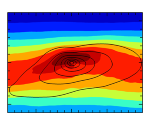
Figures 5( $a$) and 5(
 $b$) show two-dimensional conditionally averaged velocity and production based on the condition of
  $u^{\prime \prime }<-0.15\Delta U$ at convective Mach numbers
  $M_c= 0.2$ and
  $1.8$. The velocity is normalized by
  $\Delta U$. The conditionally averaged streamwise velocity
  $\breve {u}_{n}/\Delta U$ (solid lines) demonstrates elongated forward-leaning LSSs, extending a distance of
  $2\delta _\omega$ in the streamwise direction. These structures exhibit a strong negative correlation with the conditionally averaged vertical velocity
  $\breve {v}_{n}/\Delta U$ (dashed lines), indicating that low-speed LSSs are predominantly moving upwards. The spatial distribution of the production is inherently similar to the shape of the LSSs, confirming that LSSs contribute favourably to the turbulence production. The production mainly occurs at the centre of the LSSs, and decreases as the convective Mach number increases from
  $M_c= 0.2$ to
  $1.8$.

Figure 5. Two-dimensional conditionally averaged production  $\breve {P}_{n}/\bar {\epsilon }_{c}$ (contours), streamwise velocity
  $\breve {u}_{n}/\Delta U$ (solid lines) and vertical velocity
  $\breve {v}_{n}/\Delta U$ (dashed lines), and based on low-speed events with
  $u^{\prime \prime }<-0.15\Delta U$ at (
 $a$)
$a$)  $M_c=0.2$, (
 $b$)
$b$)  $M_c=1.8$. Conditionally averaged negative component of production
  $\breve {P}^-_{n}/\bar {\epsilon }_{c}$ at (
 $c$)
$c$)  $M_c=0.2$, (
 $d$)
$d$)  $M_c=1.8$.
We decompose the kinetic energy production  ${P}$ into a positive component
  ${P}^+$ and a negative component
  ${P}^-$:
  ${P}={P}^+ + {P}^-$. Here,
  ${P}^+ = 0.5(P+|P|)$ and
  ${P}^- = 0.5(P-|P|)$. The positive production is contributed by negative Reynolds shear stress corresponding to Q2 and Q4 events (or ejection and sweep events) in quadrant analysis, while the negative production is contributed by positive Reynolds shear stress corresponding to Q1 and Q3 events (or positive quadrant events) (Pope Reference Pope2000; Wallace Reference Wallace2016). On average, the low-speed LSSs move upwards, and the high-speed LSSs move downwards; namely, they contribute most of the positive kinetic energy production. In figures 5(
 $c$) and 5(
 $d$), we present the conditionally averaged negative component of production
  $\breve {P}^-_{n}/\bar {\epsilon }_{c}$, which is significantly smaller than the total production
  $\breve {P}_{n}/\bar {\epsilon }_{c}$. At
  $M_c=0.2$, negative production events are mainly concentrated within the upper-right region of the low-speed LSSs. Conversely, at
  $M_c=1.8$, these negative production events primarily emerge within the lower-left region of the low-speed LSSs.
4.3. Dissipation
Figure 6( $a$) shows the contribution of low-speed LSSs to the dissipation of turbulent kinetic energy
  $\bar {\epsilon }_{n}/\bar {\epsilon }_{c}$ at convective Mach numbers
  $M_c= 0.2$,
  $0.8$,
  $1.8$. The dissipation contribution of low-speed LSS
  $\bar {\epsilon }_{n}/\bar {\epsilon }_{c}$ is unimodal peaking around
  $y/\delta _\omega \approx 0.1$. This observation indicates that the dissipation induced by low-speed LSSs tends towards the upper portion of the mixing layer. Unlike the contribution of low-speed LSSs to the production term,
  $\bar {\epsilon }_{n}/\bar {\epsilon }_{c}$ remains non-zero near the edge of the mixing layer, extending until
  $y/\delta _\omega >0.8$ or
  $y/\delta _\omega <-0.8$. In the profile of conditionally averaged dissipation
  $\hat {\epsilon }_{n}/\bar {\epsilon }_{c}$, the dissipation near the edge of the mixing layer is significantly amplified, as shown in figure 6(
 $b$). It is evident that in regions
  $-1.0 < y/\delta _\omega < -0.5$ and
  $0.5 < y/\delta _\omega < 1.0$, there are noticeable bumps in
  $\hat {\epsilon }_{n}/\bar {\epsilon }_{c}$, with the bump being more prominent in the upper region. This observation confirms that the amplification of turbulent kinetic energy near the edges of the mixing layer is due to small-scale structures, as shown in figures 3(
 $d$)–3(
 $f$). As the convective Mach number increases, these bumps of
  $\hat {\epsilon }_{n}/\bar {\epsilon }_{c}$ rapidly decrease but still persist.

Figure 6. ( $a$) Contributions of the low-speed LSSs to dissipation
  $\bar {\epsilon }_{n}/\bar {\epsilon }_{c}$ and (
 $b$) conditionally averaged dissipation
  $\hat {\epsilon }_{n}/\bar {\epsilon }_{c}$ based on low-speed events with
  $u^{\prime \prime }<0$ at
  $M_c=0.2$,
  $0.8$ and
  $1.8$. (
 $c$)
$c$)  $\bar {\epsilon }_{n}$ is normalized by
  $\rho _\infty \Delta U^3/\delta _\omega$ with the error bar representing discrepancy among the maximum and minimum dissipation components.
When normalized by  $\rho _\infty \Delta U^3/\delta _\omega$, the dissipation decreases rapidly with increasing convective Mach number, as shown in figure 6(
 $c$). This trend is in good agreement with previous results reported by Vaghefi (Reference Vaghefi2014). However, Pantano & Sarkar (Reference Pantano and Sarkar2002) reported that the dissipation changes relatively little with varying convective Mach numbers. The error bar in figure 6(
 $a$) represents the discrepancy between the streamwise and vertical dissipation components, with each representing the maximum and minimum dissipation component, respectively. It is clear to see that the dissipation becomes more anisotropic in component as the convective Mach number increases from
  $M_c= 0.2$ to
  $1.8$, indicating the anisotropic suppression effect of compressibility on the mixing process.
Figure 7 shows two-dimensional conditionally averaged dissipation  $\breve {\epsilon }_{i,{n}}/\bar {\epsilon }_{c}$ and streamwise velocity
  $\breve {u}_{n}/\Delta U$ based on the condition of
  $u^{\prime \prime }<-0.15\Delta U$ at convective Mach numbers
  $M_c= 0.2$ and
  $1.8$. The dissipation concentrates in the upper regions of the low-speed LSSs due to the modulation effect exerted by the LSSs on the small-scale structures, wherein the small-scale vortical structures are activated at the top of low-speed LSSs. This modulation effect was initially identified and extensively studied in wall turbulence (Marusic et al. Reference Marusic, Mathis and Hutchins2010; Pirozzoli & Bernardini Reference Pirozzoli and Bernardini2011; Chan & Chin Reference Chan and Chin2022) and was observed in compressible mixing layers (Wang et al. Reference Wang, Wang and Chen2022). At
  $M_c=0.2$, the dissipation is concentrated in the upper part of the LSSs, exhibiting downstream skewness along the flow, with similar distributions and strengths across its components. At
  $M_c=1.8$, dissipation within the LSSs exhibits noticeable component anisotropy. The dissipation in the flow direction predominates significantly over the other two components, while the spanwise component remains intermediate, and the vertical component is the smallest.

Figure 7. Two-dimensional conditionally averaged components of dissipation  $\breve {\epsilon }_{i,{n}}/\bar {\epsilon }_{c}$ (contours) and streamwise velocity
  $\breve {u}_{n}/\Delta U$ (solid lines) based on low-speed events with
  $u^{\prime \prime }<-0.15\Delta U$ at (
 $a$–
$a$– $c$)
$c$)  $M_c=0.2$ and (
 $d$–
$d$– $f$)
$f$)  $1.8$. (a,d) Streamwise, (b,e) vertical and (c,f) spanwise components.
4.4. Conversion between kinetic and internal energies
Figure 8( $a$) shows the contribution of low-speed LSSs to the pressure-dilatation term
  $\bar {\varPhi }_{n}/\bar {\epsilon }_{c}$ at convective Mach numbers
  $M_c= 0.2$,
  $0.8$,
  $1.8$. The pressure-dilatation term represents the energy exchange between turbulent kinetic energy and internal energy, and is significantly smaller than the dissipation term. At convective Mach number
  $M_c= 0.2$, the pressure-dilatation term
  $\bar {\varPhi }_{n}/\bar {\epsilon }_{c}$ is negative almost everywhere with its minimum at
  $y/\delta _\omega = -0.2$, indicating that the mean pressure-dilatation converts turbulent kinetic energy into internal energy within the LSSs. As the convective Mach number increases from
  $M_c = 0.2$ to
  $1.8$, the magnitude of the minimum value of
  $\bar {\varPhi }_{n}/\bar {\epsilon }_{c}$ increases, and the location of this minimum shifts slightly downwards. At higher convective Mach numbers
  $M_c = 0.8$ and
  $1.8$,
  $\bar {\varPhi }_{n}/\bar {\epsilon }_{c}$ becomes positive for
  $y/\delta _\omega > 0.2$, peaking at
  $y/\delta _\omega = 0.5$. This observation implies that pressure-dilatation converts internal energy into the turbulent kinetic energy at the upper region of low-speed LSSs where the small-scale structures are concentrated. The contribution of low-speed LSSs to mean pressure-dilatation
  $\bar {\varPhi }_{n}/\bar {\epsilon }_{c}$ increases with enhanced compressibility, but it still remains almost two orders of magnitude smaller than the production and dissipation terms, and has usually been neglected in previous literature (Pantano & Sarkar Reference Pantano and Sarkar2002; Arun et al. Reference Arun, Sameen, Srinivasan and Girimaji2019).

Figure 8. ( $a$) Contributions of the low-speed LSSs to pressure-dilatation
  $\bar {\varPhi }_{n}/\bar {\epsilon }_{c}$ and (
 $b$) conditionally averaged pressure-dilatation
  $\hat {\varPhi }_{n}/\bar {\epsilon }_{c}$ based on low-speed events with
  $u^{\prime \prime }<0$ at
  $M_c=0.2$,
  $0.8$ and
  $1.8$.
However, the local pressure-dilatation can reach the same order of magnitude as the dissipation term near the edges of the mixing layer, as shown in figure 8( $b$), where the conditionally averaged pressure-dilatation term conditioned on the low-speed LSSs
  $\hat {\varPhi }_{n}/\bar {\epsilon }_{c}$ obtains a minimum of
  $-0.15$ at
  $y/\delta _\omega =0.9$ at the highest convective Mach number
  $M_c = 1.8$, even exceeding the magnitude of dissipation at the corresponding locations. It is clearly observed that at
  $M_c = 1.8$, the pressure-dilatation fluctuates significantly near the upper edge of the mixing layer. Additionally, beyond the upper edge of the mixing layer, at
  $y/\delta _\omega > 1.0$, there is still noticeable negative pressure-dilatation, whereas near the lower boundary of the mixing layer, the magnitude of pressure-dilatation is much smaller. This is likely related to the formation of shock waves. Rossmann, Mungal & Hanson (Reference Rossmann, Mungal and Hanson2002) and Zhou, He & Shen (Reference Zhou, He and Shen2012) discovered that the shock formation mechanism closely resembles the scenario of high-speed flow around a bluff body. In other words, the upward-moving low-speed LSSs act like bulges of turbulent fluid protruding into the high-speed free stream, leading to the formation of shock waves propagating outwards from the surfaces of these LSSs. The formation of shock waves results in a dramatic conversion of turbulent kinetic energy into internal energy.
4.5. Inter-component energy transfer
The pressure-strain components are responsible for redistributing turbulent kinetic energy from the streamwise direction to the vertical and spanwise directions on average in turbulent mixing layers (Pantano & Sarkar Reference Pantano and Sarkar2002; Arun et al. Reference Arun, Sameen, Srinivasan and Girimaji2019). Figures 9( $a$), 9(
 $c$) and 9(
 $e$) show the contribution of low-speed LSSs to the pressure-strain components
  $\bar {\varPhi }_{i,{n}}/\bar {\epsilon }_{c}$ at convective Mach numbers
  $M_c= 0.2$,
  $0.8$,
  $1.8$. The three pressure-strain components
  $\bar {\varPhi }_{i,{n}}/\bar {\epsilon }_{c}$ are of the same order of magnitude as the dominant budget terms including production and dissipation. The profiles of all pressure-strain components
  $\bar {\varPhi }_{i,{n}}/\bar {\epsilon }_{c}$ exhibit a unimodal shape with their peaks located in the upper half of the mixing layer, demonstrating that the contribution of the low-speed LSSs to the component redistribution of turbulent kinetic energy concentrates in the upper half of the mixing layer. The redistribution predominantly occurs within the region
  $-0.5< y/\delta _\omega <0.7$, where the streamwise component
  $\bar {\varPhi }_{1,{n}}/\bar {\epsilon }_{c}$ is negative, while both
  $\bar {\varPhi }_{2,{n}}/\bar {\epsilon }_{c}$ and
  $\bar {\varPhi }_{3,{n}}/\bar {\epsilon }_{c}$ components are positive, with their magnitudes being nearly identical to each other. This result indicates that the energy loss from the streamwise component is equally redistributed to the vertical and spanwise components.

Figure 9. ( $a$–
$a$– $c$) Contributions of the low-speed LSSs to pressure-strain
  $\bar {\varPhi }_{i,{n}}/\bar {\epsilon }_{c}$ and (
 $d$–
$d$– $f$) conditionally averaged pressure-strain
  $\hat {\varPhi }_{i,{n}}/\bar {\epsilon }_{c}$ based on low-speed events with
  $u^{\prime \prime }<0$ at
  $M_c=0.2$,
  $0.8$ and
  $1.8$. (a,d) Streamwise, (b,e) vertical and (c,f) spanwise components.
Near the edge of the mixing layer,  $\bar {\varPhi }_{i,{n}}/\bar {\epsilon }_{c}$ is obviously non-zero for
  $y/\delta _\omega < -0.5$ and
  $y/\delta _\omega > 0.7$. Similar to the dissipation, the volume fraction corresponding to the pressure redistribution process near the mixing layer edge is small, but the magnitude of the pressure-strain components is not negligible. This is evident in the conditionally averaged pressure-strain components
  $\hat {\varPhi }_{i,{n}}/\bar {\epsilon }_{c}$ shown in figures 9(
 $d$)–9(
 $f$). Within region
  $-1.0 < y/\delta _\omega < -0.5$, both
  $\hat {\varPhi }_{1,{n}}/\bar {\epsilon }_{c}$ and
  $\hat {\varPhi }_{3,{n}}/\bar {\epsilon }_{c}$ exhibit a negative peak, while
  $\hat {\varPhi }_{2,{n}}/\bar {\epsilon }_{c}$ shows a positive peak, even reaching twice the magnitude of its peak observed in the central region of the mixing layer at low convective Mach number
  $M_c= 0.2$. These peaks are all located around
  $y/\delta _\omega \approx -0.85$. The observation indicates that both streamwise and spanwise turbulent kinetic energy are simultaneously converted to the vertical direction near the edge of the mixing layer. This can be attributed to the dynamics of the TNTI. A key characteristic of the TNTI is the well-known vorticity jump (or strong velocity gradient) across the interface, which resembles a shear layer that can become unstable under certain conditions. This unstable shear layer can cause the formation of secondary Kelvin–Helmholtz instabilities, which are linked to the nibbling process at the TNTI (Philip et al. Reference Philip, Meneveau, de Silva and Marusic2014; Reuther & Kähler Reference Reuther and Kähler2020). The secondary Kelvin–Helmholtz instabilities redistribute turbulent kinetic energy by converting the horizontal components into the vertical component. Similarly, at the upper edge of the mixing layer, within the region
  $0.5 < y/\delta _\omega < 1.0$, the exchange of streamwise and spanwise turbulent kinetic energy to the normal direction also occurs, albeit with relatively weaker intensity. It is interesting to note that the peaks of the conditionally averaged pressure-strain
  $\hat {\varPhi }_{i,{n}}/\bar {\epsilon }_{c}$ near the edges of the mixing layer rapidly decrease with the increase in convective Mach number, whereas the peaks in the central region of the mixing layer remain insensitive to the convective Mach number. This observation may be due to the fact that the pressure redistribution process occurs at both large and small scales. The large scales contribute more significantly to the overall redistribution, while the small scales exhibit more intense activity (Lee & Moser Reference Lee and Moser2019; Wang et al. Reference Wang, Wang, Li and Chen2021). The increase in compressibility noticeably suppresses the pressure redistribution process associated with the small-scale structures. When normalized by
  $\rho _\infty \Delta U^3/\delta _\omega$, the pressure-strain terms exhibit a significant decrease with increasing Mach number, and are omitted here for the sake of brevity. In agreement with previous investigations, the decreasing of the pressure-strain term with increasing
  $M_c$ leads to inhibited energy redistributing from the streamwise to cross-stream fluctuations, to the reduced turbulence production and, finally, to reduced turbulence levels as well as reduced growth rate of the shear layer (Vreman et al. Reference Vreman, Sandham and Luo1996; Pantano & Sarkar Reference Pantano and Sarkar2002; Mahle Reference Mahle2007).
Figure 10 shows two-dimensional conditionally averaged pressure-strain  $\breve {\varPhi }_{i,{n}}/\bar {\epsilon }_{c}$ and velocity
  $\breve {u}_{n}/\Delta U$ based on the condition of
  $u^{\prime \prime }<-0.15\Delta U$ at convective Mach numbers
  $M_c= 0.2$ and
  $1.8$. Although, on average, energy is evenly redistributed from streamwise to vertical and spanwise directions, the shapes of
  $\breve {\varPhi }_{2,{n}}/\bar {\epsilon }_{c}$ and
  $\breve {\varPhi }_{3,{n}}/\bar {\epsilon }_{c}$ in low-speed LSSs are completely different. This observation indicates a highly non-uniform redistribution of turbulent kinetic energy from the streamwise to the vertical and spanwise directions at the same location within LSSs. Far away from the centre of low-speed LSSs and biased towards the upstream direction,
  $\breve {\varPhi }_{1,{n}}/\bar {\epsilon }_{c}$ and
  $\breve {\varPhi }_{3,{n}}/\bar {\epsilon }_{c}$ display a large-scale region with strikingly similar shapes and large magnitude. In this region,
  $\breve {\varPhi }_{1,{n}}/\bar {\epsilon }_{c}$ takes on a negative value, while
  $\breve {\varPhi }_{3,{n}}/\bar {\epsilon }_{c}$ is positive. Thus, the streamwise turbulent kinetic energy
  $K_1$ is predominantly redistributed to the spanwise direction
  $K_3$. Near the centre of the LSSs and in a smaller region located above, there is a significant transfer of energy from
  $K_1$ to
  $K_2$, as shown in figures 10(
 $b$) and 10(
 $e$). Below the centre of the LSSs, at
  $(r_x/\delta _\omega, r_y/\delta _\omega )\approx (0.0,-0.2)$,
  $\breve {\varPhi }_{3,{n}}/\bar {\epsilon }_{c}$ is negative, while
  $\breve {\varPhi }_{1,{n}}/\bar {\epsilon }_{c}$ and
  $\breve {\varPhi }_{2,{n}}/\bar {\epsilon }_{c}$ are positive, with relatively small magnitudes. Therefore, a small portion of turbulent kinetic energy is redistributed from
  $K_3$ to
  $K_1$ and
  $K_2$, primarily to
  $K_2$. The non-uniform redistribution shown in figures 9 and 10 is related to the pressure response caused by different scales. In the central region of the mixing layer, energy redistribution primarily occurs at larger scales, where the streamwise turbulent kinetic energy is transferred into the spanwise and vertical directions. Near the edges of the mixing layer, energy redistribution takes place at smaller scales, where turbulent kinetic energy shifts from the streamwise and spanwise components to the vertical component.

Figure 10. Two-dimensional conditionally averaged components of pressure-strain  $\breve {\varPhi }_{i,{n}}/\bar {\epsilon }_{c}$ (contours) and streamwise velocity
  $\breve {u}_{n}/\Delta U$ (solid lines) based on low-speed events with
  $u^{\prime \prime }<-0.15\Delta U$ at (
 $a$–
$a$– $c$)
$c$)  $M_c=0.2$ and (
 $d$–
$d$– $f$)
$f$)  $1.8$. (a,d) Streamwise, (b,e) vertical and (c,f) spanwise components.
To further investigate the turbulent kinetic energy exchange among different components, we decompose the pressure-strain terms into positive and negative components:  $\varPhi _i=\varPhi ^+_i + \varPhi ^-_i$, where the positive component
  $\varPhi _i^+ = 0.5(\varPhi _i+|\varPhi _i|)$ and the negative component
  $\varPhi ^-_i = 0.5(\varPhi _i-|\varPhi _i|)$. The two-dimensional conditionally average of the positive and negative pressure-strain components are shown in figures 11 and 12 for
  $M_c=0.2$ and
  $1.8$, respectively. At low Mach number
  $M_c=0.2$, the contours of
  $\breve {\varPhi }^+_{i,{n}}/\bar {\epsilon }_{c}$ and
  $\breve {\varPhi }^-_{i,{n}}/\bar {\epsilon }_{c}$ exhibit strikingly similar shapes, featuring a maximum value skewed towards the upper right side of the LSSs, with
  $\breve {\varPhi }^+_{1,{n}}/\bar {\epsilon }_{c}$ having smaller magnitude. This observation indicates that each turbulent kinetic energy component not only receives energy from the other two directions, but also contributes energy to them simultaneously. At high Mach number
  $M_c=1.8$, the magnitudes of
  $\breve {\varPhi }^+_{i,{n}}/\bar {\epsilon }_{c}$ and
  $\breve {\varPhi }^-_{i,{n}}/\bar {\epsilon }_{c}$ decrease and become more anisotropic compared with that at
  $M_c=0.2$. Here,
  $\breve {\varPhi }^-_{1,{n}}/\bar {\epsilon }_{c}$,
  $\breve {\varPhi }^+_{2,{n}}/\bar {\epsilon }_{c}$ and
  $\breve {\varPhi }^+_{3,{n}}/\bar {\epsilon }_{c}$ display two distinct peak regions in their contours, and are significantly larger than their respective counterparts. The transfer of energy from
  $K_1$ to
  $K_2$ predominantly occurs in a smaller-scale region at the upper right of the large-scale centre (at
  $r_x=0, r_y=0$), while the transfer from
  $K_1$ to
  $K_3$ takes place in a larger-scale region to the upper left of the large-scale centre. The exchange of turbulent kinetic energy between other components is notably reduced at
  $M_c=1.8$.

Figure 11. Two-dimensional conditionally averaged ( $a$–
$a$– $c$) positive part of pressure-strain
  $\breve {\varPhi }^+_{i,{n}}/\bar {\epsilon }_{c}$, (
 $d$–
$d$– $f$) negative part of pressure-strain
  $\breve {\varPhi }^-_{i,{n}}/\bar {\epsilon }_{c}$ (contours) and streamwise velocity
  $\breve {u}_{n}/\Delta U$ (solid lines) based on low-speed events with
  $u^{\prime \prime }<-0.15\Delta U$ at
  $M_c=0.2$. (a,d) Streamwise, (b,e) vertical and (c,f) spanwise components.

Figure 12. Two-dimensional conditionally averaged ( $a$–
$a$– $c$) positive part of pressure-strain
  $\breve {\varPhi }^+_{i,{n}}/\bar {\epsilon }_{c}$, (
 $d$–
$d$– $f$) negative part of pressure-strain
  $\breve {\varPhi }^-_{i,{n}}/\bar {\epsilon }_{c}$ (contours) and streamwise velocity
  $\breve {u}_{n}/\Delta U$ (solid lines) based on low-speed events with
  $u^{\prime \prime }<-0.15\Delta U$ at
  $M_c=1.8$. (a,d) Streamwise, (b,e) vertical and (c,f) spanwise components.
4.6. Spatial diffusion
Figures 13( $a$)–13(
 $c$) show the contribution of low-speed LSSs to the turbulent diffusion of turbulent kinetic energy
  $\bar {T}_{t,i,{n}}/\bar {\epsilon }_{c}$ at convective Mach numbers
  $M_c= 0.2$,
  $0.8$,
  $1.8$. Turbulent diffusion exhibits a clear anisotropy. The streamwise component of turbulent diffusion is the largest, followed by the vertical component and the spanwise component is the smallest. The contribution of low-speed LSSs to the streamwise turbulent diffusion term,
  $\bar {T}_{t,1,{n}}/\bar {\epsilon }_{c}$, resembles a wave shape, with a phase shift upwards by approximately
  $0.15/\delta _\omega$. The peak of this wave is located at
  $y/\delta _\omega = 0.4$, while the trough is positioned around
  $y/\delta _\omega = -0.15$. This observation indicates that within low-speed LSSs,
  $\bar {T}_{t,1,{n}}/\bar {\epsilon }_{c}$ transports streamwise turbulent kinetic energy
  $K_1$ upwards, whereas within high-speed LSSs, it transports
  $K_1$ downwards (not shown). It is interesting to note that the growth of
  $\bar {T}_{t,1,{n}}/\bar {\epsilon }_{c}$ from its trough to peak is nearly linear. Unlike the streamwise component, the vertical component of turbulent diffusion
  $\bar {T}_{t,2,{n}}/\bar {\epsilon }_{c}$ transports vertical turbulent kinetic energy
  $K_2$ from the centre of the mixing layer to both the upper and lower edges of the mixing layer simultaneously, although the downward transport is relatively minor. The spanwise component of turbulent diffusion
  $\bar {T}_{t,3,{n}}/\bar {\epsilon }_{c}$, however, behaves similarly to the vertical component, as it transports spanwise turbulent kinetic energy
  $K_3$ from the centre of the mixing layer to both the upper and lower edges of the mixing layer.

Figure 13. ( $a$–
$a$– $c$) Contributions of the low-speed LSSs to turbulent diffusion
  $\bar {T}_{t,i,{n}}/\bar {\epsilon }_{c}$ and (
 $d$–
$d$– $f$) conditionally averaged turbulent diffusion
  $\hat {T}_{t,i,{n}}/\bar {\epsilon }_{c}$ based on low-speed events with
  $u^{\prime \prime }<0$ at
  $M_c=0.2$,
  $0.8$ and
  $1.8$. (a,d) Streamwise, (b,e) vertical and (c,f) spanwise components.
The conditionally averaged turbulent diffusion term  $\hat {T}_{t,i,{n}}/\bar {\epsilon }_{c}$ is presented in figures 13(
 $d$)–13(
 $f$), where the local turbulent diffusion process is highlighted at the edges of the mixing layer. Here,
  $\hat {T}_{t,1,{n}}/\bar {\epsilon }_{c}$ peaks at
  $y/\delta _\omega = 0.7$, with an additional small trough appearing at
  $y/\delta _\omega = -0.7$. Additionally,
  $\hat {T}_{t,1,{n}}/\bar {\epsilon }_{c}$ exhibits linear growth from its minimum to maximum values. At
  $M_c = 0.2$ and
  $0.8$, the range of this linear growth region expands to almost
  $y/\delta _\omega = 0.7$. Furthermore, the range of linear growth widens with decreasing convective Mach number, in contrast to the behaviour of the linear stage of volume fraction, as shown in figure 2(
 $a$). The two peaks of
  $\hat {T}_{t,2,{n}}/\bar {\epsilon }_{c}$ and
  $\hat {T}_{t,3,{n}}/\bar {\epsilon }_{c}$ have shifted to
  $y/\delta _\omega = \pm 0.8$. The vertical variation of
  $\hat {T}_{t,2,{n}}/\bar {\epsilon }_{c}$ is very large, especially at the edges of the mixing layer, where its peak near the upper edge even exceeds the peak of
  $\hat {T}_{t,1,{n}}/\bar {\epsilon }_{c}$. The magnitude of
  $\hat {T}_{t,3,{n}}/\bar {\epsilon }_{c}$ is noticeably smaller than the other two components. As the convective Mach number increases, the conditionally averaged turbulent diffusion term
  $\hat {T}_{t,i,{n}}/\bar {\epsilon }_{c}$ decreases rapidly near the edges of the mixing layer, while it remains relatively unchanged at the centre of the mixing layer.
More insight into the spatial distribution of the turbulent diffusion can be gained from its two-dimensional conditional average shown in figure 14. The streamwise turbulent diffusion features two large-scale regions of similar shapes, with positive values in the upper left and negative values in the lower right. This suggests that the streamwise turbulent diffusion  $\breve {T}_{t,1,{n}}/\bar {\epsilon }_{c}$ transports streamwise turbulent kinetic energy from the lower right region of the low-speed LSSs to its upper left region. In other words, the direction of turbulent diffusion of
  $K_1$ is not vertical but inclined, with a skew angle of approximately
  $18^\circ$ at
  $M_c= 0.2$ and
  $15^\circ$ at
  $1.8$. This angle is measured between the line (black dashed line figure 14a,d) connecting the extrema (maximum and minimum points) of the two large-scale regions and the horizontal direction. The direction of turbulent diffusion
  $K_2$ also tends to be from the lower right region of the LSSs towards its upper left region, but with a weaker intensity. However, the direction of turbulent diffusion
  $K_3$ tends to be from the upper left region of the LSSs towards its lower right region, opposite to the direction of
  $K_1$ and
  $K_2$. The inclined distribution of the turbulent diffusion components in the
  $x\unicode{x2013}y$ plane causes positive and negative values to cancel each other out when averaged in the horizontal plane. As a result, the maximum positive and negative values of the turbulent diffusion components in the two-dimensional average shown in figure 14 are significantly larger than their counterparts in figures 13(
 $d$)–13(
 $f$), especially for the streamwise component of turbulent diffusion.

Figure 14. Two-dimensional conditionally averaged components of turbulent diffusion  $\breve {T}_{t,i,{n}}/\bar {\epsilon }_{c}$ (contours) and streamwise velocity
  $\breve {u}_{n}/\Delta U$ (solid lines) based on low-speed events with
  $u^{\prime \prime }<-0.15\Delta U$ at (
 $a$–
$a$– $c$)
$c$)  $M_c=0.2$ and (
 $d$–
$d$– $f$)
$f$)  $1.8$. (a,d) Streamwise, (b,e) vertical and (c,f) spanwise components.
Figures 15( $a$)–15(
 $c$) show the contribution of low-speed LSSs to the pressure diffusion of turbulent kinetic energy
  $\bar {T}_{p,i,{n}}/\bar {\epsilon }_{c}$ at convective Mach numbers
  $M_c= 0.2$,
  $0.8$,
  $1.8$. Compared with the turbulent diffusion, the value of pressure diffusion is much smaller. The magnitudes of the three components of pressure diffusion
  $\bar {T}_{p,i,{n}}/\bar {\epsilon }_{c}$ are comparable. The contribution of low-speed LSSs to the streamwise component of pressure diffusion
  $\bar {T}_{p,1,{n}}/\bar {\epsilon }_{c}$ also exhibits a wave shape, with its peak at
  $y/\delta _\omega = - 0.5$ and its trough at
  $y/\delta _\omega = 0.2$. Thus, it transports streamwise turbulent kinetic energy
  $K_1$ from the upper to the lower part of the mixing layer, in contrast to the role of
  $\bar {T}_{t,1,{n}}/\bar {\epsilon }_{c}$. The vertical pressure diffusion term
  $\bar {T}_{p,2,{n}}/\bar {\epsilon }_{c}$ exhibits a positive peak located at
  $y/\delta _\omega \approx 0$, flanked by negative peaks on either side, with the upper negative peak stronger than the lower one, indicating that
  $\bar {T}_{p,2,{n}}/\bar {\epsilon }_{c}$ transports vertical turbulent kinetic energy
  $K_2$ from the edges of the mixing layer towards its centre, in contrast to the role of
  $\bar {T}_{t,2,{n}}/\bar {\epsilon }_{c}$. The distribution of
  $\bar {T}_{p,3,{n}}/\bar {\epsilon }_{c}$ along the
  $y$-direction is relatively complex, with its sign changing multiple times. In the range of
  $-0.7< y/\delta _\omega < 0.5$,
  $\bar {T}_{p,3,{n}}/\bar {\epsilon }_{c}$ primarily transports
  $K_3$ from the upper to lower part of the mixing layer.

Figure 15. ( $a$–
$a$– $c$) Contributions of the low-speed LSSs to pressure diffusion
  $\bar {T}_{p,i,{n}}/\bar {\epsilon }_{c}$ and (
 $d$–
$d$– $f$) conditionally averaged pressure diffusion
  $\hat {T}_{p,i,{n}}/\bar {\epsilon }_{c}$ based on low-speed events with
  $u^{\prime \prime }<0$ at
  $M_c=0.2$,
  $0.8$ and
  $1.8$. (a,d) Streamwise, (b,e) vertical and (c,f) spanwise components.
The conditionally averaged pressure diffusion term  $\hat {T}_{p,i,{n}}/\bar {\epsilon }_{c}$ is presented in figures 15(
 $d$)–15(
 $f$), where the local pressure diffusion process is highlighted at the edges of the mixing layer. Here,
  $\hat {T}_{p,1,{n}}/\bar {\epsilon }_{c}$ peaks at
  $y/\delta _\omega = -0.8$. Additionally,
  $\hat {T}_{p,2,{n}}/\bar {\epsilon }_{c}$ is nearly symmetric about
  $y/\delta _\omega = 0$, exhibiting two remarkable negative peaks at
  $y/\delta _\omega = \pm 0.8$, with their magnitudes nearly equivalent to the maximum peak of
  $\hat {T}_{t,2,{n}}/\bar {\epsilon }_{c}$ (shown in figure 13
 $e$). At the edges of the mixing layer,
  $\hat {T}_{p,3,{n}}/\bar {\epsilon }_{c}$ exhibits two positive peaks, which are slightly larger than the two peaks of
  $\hat {T}_{t,3,{n}}/\bar {\epsilon }_{c}$ (shown in figure 13
 $f$) at the edges. As the convective Mach number increases, the conditionally averaged pressure diffusion term
  $\hat {T}_{p,i,{n}}/\bar {\epsilon }_{c}$ decreases rapidly near the edges of the mixing layer.
Figure 16 presents the two-dimensional conditional average of the pressure diffusion  $\breve {T}_{p,i,{n}}/\bar {\epsilon }_{c}$ at
  $M_c=0.2$ and
  $1.8$. On the left side of the centre of low-speed LSSs, there exists a large-scale region where the streamwise component of pressure diffusion is negative, while on the right side, there is a large-scale region with positive streamwise pressure diffusion. The black dashed line connecting the extrema (maximum and minimum points) of the two large-scale regions is almost horizontal, as shown in figures 16(
 $a$) and 16(
 $d$). This suggests that within low-speed LSSs, the streamwise pressure diffusion component
  $\breve {T}_{p,1,{n}}/\bar {\epsilon }_{c}$ primarily transports
  $K_1$ from left to right, and its non-uniformity nearly leads to the transport of
  $K_1$ from top to bottom, as shown in figure 15(
 $a$). The distribution of streamwise pressure diffusion components in the
  $x\unicode{x2013}y$ plane leads to a more pronounced effect of positive and negative values cancelling each other out when averaged in the horizontal plane. The two-dimensional distributions of the vertical and spanwise components of pressure diffusion are relatively complex, but the overall trend is to transport the vertical and spanwise turbulent kinetic energy downwards. At higher convective Mach number
  $M_c=1.8$, the pressure diffusion occurs within a smaller region.

Figure 16. Two-dimensional conditionally averaged components of pressure diffusion  $\breve {T}_{p,i,{n}}/\bar {\epsilon }_{c}$ (contours) and streamwise velocity
  $\breve {u}_{n}/\Delta U$ (solid lines) based on low-speed events with
  $u^{\prime \prime }<-0.15\Delta U$ at (
 $a$–
$a$– $c$)
$c$)  $M_c=0.2$ and (
 $d$–
$d$– $f$)
$f$)  $1.8$. (a,d) Streamwise, (b,e) vertical and (c,f) spanwise components.
The three components of viscous diffusion  $\bar {T}_{v,i,{n}}$ are each an order of magnitude smaller than turbulent diffusion and pressure diffusion across all three convective Mach numbers; therefore, they are not further analysed here for brevity.
4.7. Mass flux coupling
According to the definition of the mass flux coupling term (3.3f), its ensemble average is very small because the Favre average of  $u^{\prime \prime }$ is zero (Pantano & Sarkar Reference Pantano and Sarkar2002). The conditional averages of
  $u^{\prime \prime }$ and
  $v^{\prime \prime }$ are of the order of
  $\Delta U$, as shown in figures 5(
 $a$) and 5(
 $b$), while the conditional average of
  $w^{\prime \prime }$ remains negligible. Consequently, the conditional average of the mass flux coupling term within LSSs is not zero. Figures 17(a) and (17b) show the contribution of low-speed LSSs to the mass flux coupling term
  $\bar {\varSigma }_{i,{n}}/\bar {\epsilon }_{c}$ at convective Mach numbers
  $M_c= 0.2$,
  $0.8$,
  $1.8$. The contribution of low-speed LSSs to the streamwise mass flux coupling term
  $\bar {\varSigma }_{1,{n}}/\bar {\epsilon }_{c}$ exhibits a positive peak at
  $y/\delta _\omega =-0.25$ and it displays a negative trough at
  $y/\delta _\omega =0.25$, with the magnitudes of its peak and trough being almost equal. Considering the symmetry of high- and low-speed LSSs,
  $\bar {\varSigma }_{1,{p}}/\bar {\epsilon }_{c}$ and
  $\bar {\varSigma }_{1,{n}}/\bar {\epsilon }_{c}$ are symmetrical about the origin point, which means that they nearly cancel each other out, resulting in
  $\bar {\varSigma }_{1}$ being nearly zero. The characteristics of
  $\bar {\varSigma }_{2,{n}}/\bar {\epsilon }_{c}$ are very similar to those of
  $\bar {\varSigma }_{1,{n}}/\bar {\epsilon }_{c}$, except the magnitudes of the peaks and troughs are somewhat smaller. These results indicate that
  $\bar {\varSigma }_{1,{n}}/\bar {\epsilon }_{c}$ and
  $\bar {\varSigma }_{2,{n}}/\bar {\epsilon }_{c}$ transport streamwise and vertical turbulent kinetic energy downwards, respectively.

Figure 17. (a,b) Contributions of the low-speed LSSs to mass flux coupling  $\bar {\varSigma }_{i,{n}}/\bar {\epsilon }_{c}$ and (c,d) conditionally averaged mass flux coupling
  $\hat {\varSigma }_{i,{n}}/\bar {\epsilon }_{c}$ based on low-speed events with
  $u^{\prime \prime }<0$ at
  $M_c=0.2$,
  $0.8$ and
  $1.8$. (a,c) Streamwise and (b,d) vertical components.
The conditionally averaged mass flux coupling term  $\hat {\varSigma }_{i,{n}}/\bar {\epsilon }_{c}$ is presented in figures 17(
 $c$) and 17(
 $d$). The trough values of
  $\hat {\varSigma }_{i,{n}}/\bar {\epsilon }_{c}$ are slightly larger than the peak values. At the edges of the mixing layer, the local values of the mass flux coupling term do not exhibit significant amplification, unlike the other budget terms. Here,
  $\hat {\varSigma }_{2,{n}}/\bar {\epsilon }_{c}$ shows a minor trough near the lower edge, indicating a small amount of vertical turbulent kinetic energy is transported upwards into the turbulent region. The spanwise mass flux coupling term is negligible and is omitted here for the sake of brevity. Figure 18 shows two-dimensional conditionally averaged mass flux coupling
  $\breve {\varSigma }_{i,{n}}/\bar {\epsilon }_{c}$ based on the condition of
  $u^{\prime \prime }<-0.15\Delta U$ at convective Mach numbers
  $M_c= 0.2$ and
  $1.8$. Both the streamwise and vertical components of mass flux coupling exhibit a relatively strong negative region in the upper part of the LSSs and a weaker positive region in the lower part, qualitatively consistent with figures 17(
 $c$) and 17(
 $d$).
$d$).

Figure 18. Two-dimensional conditionally averaged mass flux coupling  $\breve {\varSigma }_{i,{n}}/\bar {\epsilon }_{c}$ (contours) and streamwise velocity
  $\breve {u}_{n}/\Delta U$ (solid lines) based on low-speed events with
  $u^{\prime \prime }<-0.15\Delta U$ at (a,b)
  $M_c=0.2$ and (c,d)
  $1.8$. (a,c) Streamwise and (b,d) vertical components.
4.8. Total variation of turbulent kinetic energy in LSSs
Figures 19( $a$)–19(
 $c$) show the contribution of low-speed LSSs to the total variation of turbulent kinetic energy,
  $\bar {V}_{i,{n}}/\bar {\epsilon }_{c}$, at convective Mach numbers
  $M_c= 0.2$,
  $0.8$,
  $1.8$. The contribution of low-speed LSSs to the total variation of streamwise turbulent kinetic energy
  $\bar {V}_{1,{n}}/\bar {\epsilon }_{c}$ exhibits two distinct positive peaks: a larger one in the upper half and a smaller one in the lower half of the mixing layer. Additionally,
  $\bar {V}_{2,{n}}/\bar {\epsilon }_{c}$ exhibits a distinct double-peak distribution, while
  $\bar {V}_{3,{n}}/\bar {\epsilon }_{c}$ shows a positive peak only in the upper half of the mixing layer and is nearly zero in the lower half. Near the centre of the mixing layer,
  $\bar {V}_{2,{n}}/\bar {\epsilon }_{c}$ and
  $\bar {V}_{3,{n}}/\bar {\epsilon }_{c}$ are almost zero, whereas
  $\bar {V}_{1,{n}}/\bar {\epsilon }_{c}$ shows a small negative value, indicating a reduction in streamwise turbulent kinetic energy
  $K_1$ at this position. This suggests that even at the centre, the mixing layer has not achieved a completely self-similar state. As the convective Mach number increases,
  $\bar {V}_{i,{n}}/\bar {\epsilon }_{c}$ decreases and the peak of
  $\bar {V}_{2,{n}}/\bar {\epsilon }_{c}$ in the lower half almost disappears at
  $M_c= 1.8$.

Figure 19. ( $a$–
$a$– $c$) Contributions of the low-speed LSSs to the total variation of turbulent kinetic energy
  $\bar {V}_{i,{n}}/\bar {\epsilon }_{c}$ and (
 $d$–
$d$– $f$) conditionally averaged total variation
  $\hat {V}_{i,{n}}/\bar {\epsilon }_{c}$ based on low-speed events with
  $u^{\prime \prime }<0$ at
  $M_c=0.2$,
  $0.8$ and
  $1.8$. (a,d) Streamwise, (b,e) vertical and (c,f) spanwise components.
The conditionally averaged total variation  $\hat {V}_{i,{n}}/\bar {\epsilon }_{c}$ is presented in figures 15(
 $d$)–15(
 $f$). Near the upper edge of the mixing layer, the total variation of
  $K_1$ is very prominent, with a peak at
  $y/\delta _\omega \approx 0.7$. In contrast, near the lower edge, the total variation of
  $K_1$ is nearly zero and surprisingly negative at
  $M_c = 0.2$. The total variations of
  $K_2$ and
  $K_3$ both exhibit significant positive peaks near both edges of the mixing layer, with the peak at the upper edge being larger. The total variation of
  $K_2$ near the upper edge, at
  $y/\delta _\omega \approx 0.7$, is particularly notable, even exceeding the value of
  $K_1$. As the convective Mach number increases, the total variations of turbulent kinetic energy in all three directions decrease significantly at the edges. These results further confirm the amplitude modulation effect of LSSs on small-scale structures at the edges of the mixing layer, consistent with the findings shown in figures 3(
 $d$)–3(
 $f$). The level of amplitude modulation is strongest for the vertical velocity, followed by the streamwise velocity and weakest for the spanwise velocity. Additionally, the amplitude modulation decreases significantly with increasing Mach number. The entrainment process is usually associated with two mechanisms: nibbling, which is considered to be carried out by small-scale structures and plays the main role, and engulfment, which is mostly due to large-scale eddies (Westerweel et al. Reference Westerweel, Fukushima, Pedersen and Hunt2005; da Silva et al. Reference da Silva, Hunt, Eames and Westerweel2014; Jahanbakhshi & Madnia Reference Jahanbakhshi and Madnia2016). We infer that with increasing convective Mach number, the level of amplitude modulation decreases significantly, resulting in weakened small-scale structures near the edge of the mixing layer. This leads to an evident increase in the normalized Kolmogorov length scale
  $\eta /\delta _\omega$, indicating a reduction in scale separation, as reported by Wang et al. (Reference Wang, Guo, Wang and Chen2024). Krug et al. (Reference Krug, Holzner, Lüthi, Wolf, Kinzelbach and Tsinober2015) proposed a relationship estimating the surface area
  $A$ of the TNTI, where
  $A \propto (\eta /\delta _\omega )^{-1/3}$. Based on this relationship, we can infer that the TNTI surface area decreases as the small-scale structures weaken. The reduction in TNTI surface area, in turn, decreases the mass flow rate associated with nibbling, as reported by Jahanbakhshi & Madnia (Reference Jahanbakhshi and Madnia2016).
5. Conclusion
DNS of compressible temporally developing mixing layers have been performed to investigate the impact of LSSs on the turbulent kinetic energy budgets in physical space and to further clarify the growth suppression mechanism associated with compressibility effects. Three cases with convective Mach number,  $M_c$, from
  $0.2$ to
  $1.8$ are analysed. In the present study, high- and low-speed LSSs are identified as negative and positive regions of fluctuating streamwise velocity
  $u^{\prime \prime }$. In the core region of mixing layers, the volume fraction of low-speed LSSs decreases linearly with a coefficient of
  $0.165$ that is independent on the convective Mach number. As the convective Mach number increases, the linear region of the volume fraction extends over a broader range.
The contributions of LSSs to the turbulent kinetic energy and their budgets are evaluated by decomposing them into three parts, representing the contributions from the low-speed LSSs, high-speed LSSs and engulfed regions in the mixing layer. The contributions of low-speed LSSs on turbulent kinetic energy, production, dissipation and pressure-strain are primarily concentrated in the region slightly above the centre of the mixing layer, while those of high-speed LSSs are concentrated slightly below the centre. The spatial diffusion and mass flux coupling terms are responsible for the vertical transport of turbulent kinetic energy. In low-speed LSSs, the streamwise component of turbulent diffusion transports  $K_1$ upwards from the lower half to the upper half of the mixing layer, while the vertical and spanwise components of turbulent diffusion transport
  $K_2$ and
  $K_3$ from the middle to the edges of the mixing layer, respectively. In the core region of low-speed LSSs, the growth of streamwise turbulent diffusion is nearly linear. The pressure diffusion term acts with less intensity. The streamwise pressure diffusion transports
  $K_1$ downwards from the upper half to the lower half of the mixing layer, while the vertical and spanwise components of pressure diffusion transport
  $K_2$ and
  $K_3$ from the edges to the middle of the mixing layer, respectively. The streamwise and vertical mass flux coupling terms are comparable to the other dominant terms, and transport
  $K_1$ and
  $K_2$ downwards, respectively. The viscous diffusion and spanwise mass flux coupling terms are negligible in low-speed LSSs.
The spatial distribution of energy budget terms in low-speed LSSs is investigated through conditional averaging. The energy budgets near the edges of the mixing layer are dominated by small-scale structures. At the edges of LSSs, the sources and losses of all three components of turbulent kinetic energy are completely different to each other, and dominated by turbulent diffusion, pressure diffusion, pressure-strain and dissipation terms. In low-speed LSSs, the streamwise turbulent kinetic energy near the upper edge originates from turbulent diffusion, while near the lower edge, it comes from pressure diffusion. Most of the streamwise turbulent kinetic energy is transferred to the vertical direction through pressure-strain, and the remaining small portion is dissipated by viscous effects. The vertical turbulent kinetic energy near both edges mainly originates from turbulent diffusion, with an additional portion coming from the streamwise and spanwise directions via pressure-strain. The loss of vertical turbulent kinetic energy is primarily due to pressure diffusion, which transports it to the interior of the LSSs, with a small portion dissipated by viscous effects. The spanwise turbulent kinetic energy comes from both turbulent diffusion and pressure diffusion. Most of it is transferred to the vertical direction through pressure-strain, while a small portion is dissipated by viscous effects.
The pressure-dilatation increases rapidly with the convective Mach number, but it is still an order of magnitude smaller than other terms. In the lower part of the low-speed LSSs, pressure-dilatation is negative, indicating that turbulent kinetic energy is converted to internal energy. In the upper part, pressure-dilatation is positive, converting internal energy to turbulent kinetic energy. At  $M_c=1.8$, strong negative pressure-dilatation appears at the upper edge of the low-speed LSSs due to the formation of noticeable shock waves, which rapidly converts turbulent kinetic energy to internal energy.
Finally, the analysis of the turbulent kinetic energy budget reveals the interaction between large-scale and small-scale structures in compressible turbulent mixing layers. The turbulent kinetic energy, their total variation and dissipation are significantly amplified at two edges of the mixing layer, which supports the existence of amplitude modulation exerted by the LSSs onto the near-edge small-scale structures. The level of amplitude modulation is strongest for the vertical velocity, followed by the streamwise velocity and weakest for the spanwise velocity. Additionally, the amplitude modulation decreases significantly with increasing Mach number in compressible mixing layers. The above results are meaningful for turbulence modelling, as they suggest the potential for developing predictive models for various budget terms of turbulent kinetic energy based on the amplitude modulation effect, similar to velocity prediction model proposed by Marusic et al. (Reference Marusic, Mathis and Hutchins2010).
Funding
This work was supported by the National Natural Science Foundation of China (NSFC grants 12172161, 92052301, 12161141017 and 91952104), by the NSFC Basic Science Center Program (grant no. 11988102), by the Shenzhen Science and Technology Program (grant no. KQTD20180411143441009) and by Department of Science and Technology of Guangdong Province (grant nos 2019B21203001, 2020B1212030001, 2023B1212060001). This work was also supported by Center for Computational Science and Engineering of Southern University of Science and Technology.
Declaration of interests
The authors report no conflict of interest.
Appendix. Confinement effect of the computational domain
In this section, the confinement effect of the computational domain is investigated to validate the data. To minimize the effects of the finite domain size on the results, the two-point correlation should be small for large  $r$. Figures 20 and 21 show that this condition is satisfied for the case with
  $M_c=0.2$ and
  $M_c=1.8$, respectively.

Figure 20. ( $a$–
$a$– $c$) Streamwise and (
 $d$–
$d$– $f$) spanwise two-point correlations of (a,d) streamwise, (b,e) vertical and (c,f) spanwise velocities at the centreline at several time instants from
  $\tau =125$ to
  $\tau =750$ for the case with
  $M_c=0.2$.

Figure 21. ( $a$–
$a$– $c$) Streamwise and (
 $d$–
$d$– $f$) spanwise two-point correlations of (a,d) streamwise, (b,e) vertical and (c,f) spanwise velocities at the centreline at several time instants from
  $\tau =250$ to
  $\tau =2250$ for the case with
  $M_c=1.8$.
At  $M_c=1.8$,
  $\mathcal {R}_{xu}$ in the later part of the self-similar stage from
  $\tau =2000$ to
  $\tau =2250$ does not exhibit complete decay to zero decorrelation and
  $\mathcal {R}_{zu}$ does not return to zero after the negative correlation, as shown in figures 21(
 $a$) and 21(
 $d$), since the scale of the high- and low-speed LSSs have become comparable to the size of the computational domain. Similar behaviour has been observed in the results of Vaghefi (Reference Vaghefi2014). However, as supported by prior studies, when the magnitude of two-point correlation is sufficiently small, the confinement effect of the computational domain is insignificant, especially for one-point statistics (O'Neill et al. Reference O'Neill, Nicolaides, Honnery and Soria2004; Lozano-Durán & Jiménez Reference Lozano-Durán and Jiménez2014; Lee & Moser Reference Lee and Moser2015). Comparison of one-point statistics of turbulent kinetic energy, production and dissipation terms with different
  $\tau _f$ at
  $M_c=1.8$ are shown in figure 22. The good agreement of the results with
  $\tau _f=1750$ and
  $\tau _f=2250$ suggests that the data beyond
  $\tau _f=1750$ still accurately captures the physical processes involved. Even for the pressure-dilatation term, which is relatively sensitive to the sample size, the results with
  $\tau _f=1750$ and
  $\tau _f=2250$ are very similar, except for noticeable differences near the edges of the mixing layer, as shown in figure 22(
 $f$). Additionally, we compared the two-dimensional conditionally averaged streamwise velocity, production and dissipation terms at
  $\tau _f=1750$ and
  $\tau _f=2250$ in figure 23 for
  $M_c=1.8$. The results show that the differences between the two cases are minimal, occurring only in regions farther from the origin.

Figure 22. Comparison of one-point statistics with different  $\tau _f$ for
  $M_c=1.8$. (
 $a$–
$a$– $c$) Conditionally averaged turbulent kinetic energy
  $\hat {K}_{i,{n}}/(\rho _\infty \Delta U^2)$. (
 $d$–
$d$– $f$) Conditionally averaged production
  $\hat {P}_{n}/\bar {\epsilon }_{c}$, dissipation
  $\hat {\epsilon }_{n}/\bar {\epsilon }_{c}$ and pressure-dilatation
  $\hat {\varPhi }_{n}/\bar {\epsilon }_{c}$.

Figure 23. Comparison of two-dimensional conditionally averaged ( $a$) streamwise velocity
  $\breve {u}_{n}/\Delta U$, (
 $b$) production
  $\breve {P}_{n}/\bar {\epsilon }_{c}$ and dissipation
  $\breve {\epsilon }_{1,{n}}/\bar {\epsilon }_{c}$ with different
  $\tau _f$ for
  $M_c=1.8$.
Table 2 contains the most relevant publications of DNS of temporally developing compressible mixing layer, together with  $M_c$, the range of the self-similar period, the computational domain dimensions and the integral lengths. We can see that the largest integral length scale of
  $l_x/L_x=0.151$ is obtained at the end of the self-similar region at
  $M_c=1.8$ in the present work, and it is comparable to the previous numerical results of Vaghefi (Reference Vaghefi2014) and Yu & Lu (Reference Yu and Lu2020).
Table 2. The beginning ( $\tau =\tau _0$) and end (
 $\tau =\tau _f$) times of the self-similar period, domain lengths (
 $L_x$,
  $L_y$ and
  $L_z$) and integral lengths (
 $l_x$ and
  $l_z$) in the most relevant publications of DNS of temporally developing compressible mixing layer at higher convective Mach number. Only the integral lengths at the end time (
 $\tau =\tau _f$) of the self-similar period are presented by Pantano & Sarkar (Reference Pantano and Sarkar2002), Vaghefi (Reference Vaghefi2014), Arun et al. (Reference Arun, Sameen, Srinivasan and Girimaji2019) and Yu & Lu (Reference Yu and Lu2020).

We conclude from these results that the scale of the computational domain in this study is appropriate, and setting the end time of the self-similar period at  $\tau _f=2250$ for
  $M_c=1.8$ is reasonable. The confinement effect of the computational domain is insignificant even though the two-point correlations do not exhibit complete decay to zero decorrelation within the computational domain.


