1 Introduction
Sinusoidal oscillatory flow over two-dimensional wavy bedforms represents an idealized model for wave-induced flow over a ripple-covered seabed, a ubiquitous configuration in coastal regions. This oscillatory flow is significantly different than the flow over flat beds due to the presence of large-scale spanwise vortices. These coherent vortices are formed during each half-cycle by flow separation at ripple crests (Darwin Reference Darwin1883; Bagnold & Taylor Reference Bagnold and Taylor1946). While forming, the adverse gradients in their pressure fields give rise to secondary vortices on the ripple surface (Blondeaux & Vittori Reference Blondeaux and Vittori1991, Reference Blondeaux and Vittori1999). The resulting vortex pairs are eventually washed over the ripple crests and ejected into the free stream during the flow reversal (Nakato et al.
Reference Nakato, Kennedy, Glover and Locher1977). In this phase, the vortices can suspend considerable amounts of sediments, cf. e.g. Honji, Kaneko & Matsunaga (Reference Honji, Kaneko and Matsunaga1980), van der Werf et al. (Reference van der Werf, Ribberink, O’Donoghue and Doucette2006) and van der Werf et al. (Reference van der Werf, Doucette, O’Donoghue and Ribberink2007). Due to this prominence of vortices in the local hydrodynamics, sand ripples are usually referred to as vortex ripples (Nielsen Reference Nielsen1992). Natural vortex ripples have wavelengths of
 $O(10~\text{cm})$
(Mei & Liu Reference Mei and Liu1993), and the vortex formation and ejection events occur in fully turbulent regimes. To date, the dynamics of the flow in these regimes is not sufficiently explored in detail. This work is an effort in this direction. We perform direct numerical simulations (DNS) of sinusoidal oscillatory flow over a periodic array of two-dimensional ripples.
$O(10~\text{cm})$
(Mei & Liu Reference Mei and Liu1993), and the vortex formation and ejection events occur in fully turbulent regimes. To date, the dynamics of the flow in these regimes is not sufficiently explored in detail. This work is an effort in this direction. We perform direct numerical simulations (DNS) of sinusoidal oscillatory flow over a periodic array of two-dimensional ripples.
1.1 General properties of vortex ripples
For a specific ripple profile, the oscillatory flow around it has three essential length scales: the wave-orbital amplitude
 $A$
, the ripple wavelength
$A$
, the ripple wavelength
 $\unicode[STIX]{x1D706}$
, the ripple height
$\unicode[STIX]{x1D706}$
, the ripple height
 $\unicode[STIX]{x1D702}$
; and a time scale: the wave period
$\unicode[STIX]{x1D702}$
; and a time scale: the wave period
 $T$
, which is used to define the angular frequency
$T$
, which is used to define the angular frequency
 $\unicode[STIX]{x1D714}=2\unicode[STIX]{x03C0}/T$
. These characteristic length and time scales, together with the fluid kinematic viscosity
$\unicode[STIX]{x1D714}=2\unicode[STIX]{x03C0}/T$
. These characteristic length and time scales, together with the fluid kinematic viscosity
 $\unicode[STIX]{x1D708}$
, are conveniently merged into three dimensionless parameters: Reynolds number
$\unicode[STIX]{x1D708}$
, are conveniently merged into three dimensionless parameters: Reynolds number
 $$\begin{eqnarray}Re=\frac{A^{2}\unicode[STIX]{x1D714}}{\unicode[STIX]{x1D708}},\end{eqnarray}$$
(typically in the range
 $O(10^{4}{-}10^{5})$
), Keulegan–Carpenter number
$O(10^{4}{-}10^{5})$
), Keulegan–Carpenter number
 $$\begin{eqnarray}K_{C}=2\unicode[STIX]{x03C0}\frac{A}{\unicode[STIX]{x1D706}},\end{eqnarray}$$
giving the ratio of the ambient excursion amplitude to the ripple wavelength (typically in the range
 $O(1-10)$
) and ripple steepness
$O(1-10)$
) and ripple steepness
 $$\begin{eqnarray}s=\frac{\unicode[STIX]{x1D702}}{\unicode[STIX]{x1D706}},\end{eqnarray}$$
with typical values between 0.1 and 0.2.
A considerable amount of knowledge on the turbulent flow over vortex ripples has been obtained from laboratory experiments with rigid ripple models or sand ripples under equilibrium conditions. Table 1 presents a short bibliographical list of previous works. Sato, Mimura & Watanabe (Reference Sato, Mimura and Watanabe1985) were among the first to explore how the turbulence production and hydrodynamic forces are related to the dynamics of coherent lee vortices. Earnshaw & Greated (Reference Earnshaw and Greated1998) and Jespersen et al. (Reference Jespersen, Thomassen, Andersen and Bohr2004) characterized the oscillatory flow over rigid ripples using vorticity dynamics. To this end, they calculated the circulation, area and trajectory of the lee vortices. Fredsøe, Andersen & Sumer (Reference Fredsøe, Andersen and Sumer1999) visualized the formation and ejection sequence of the primary lee vortex, and showed that the intensity of turbulence near the ripple surface increases substantially when the lee vortex is washed over the crest. Nichols & Foster (Reference Nichols and Foster2007) studied movable sand ripples under large-scale free-surface wave conditions. They showed that the intensity of instantaneous vortical structures is correlated with the
 $K_{C}$
number. Hare et al. (Reference Hare, Hay, Zedel and Cheel2014) investigated the spatial and temporal structures of the flow over sand ripples with turbulence-resolving experiments. Besides the basic first-order flow statistics, they measured the distribution of Reynolds stresses, and the turbulent kinetic energy and its production rate.
$K_{C}$
number. Hare et al. (Reference Hare, Hay, Zedel and Cheel2014) investigated the spatial and temporal structures of the flow over sand ripples with turbulence-resolving experiments. Besides the basic first-order flow statistics, they measured the distribution of Reynolds stresses, and the turbulent kinetic energy and its production rate.
Due to resolution restrictions, the experimental measurements did not address more detailed characteristics such as the distribution of wall shear stresses over the ripple surface. These properties were predicted using large-eddy simulations (LES), e.g. Zedler & Street (Reference Zedler and Street2006) and Grigoriadis, Dimas & Balaras (Reference Grigoriadis, Dimas and Balaras2012). However, the subgrid-scale and wall models in these simulations are yet to be verified using DNS or high-resolution experimental data.
Table 1. Summary of previous studies on oscillatory flow over vortex ripples. OWT stands for oscillatory water tunnel.

a
In experiments with a single ripple, the
 $K_{C}$
number is calculated using the ripple height, i.e.
$K_{C}$
number is calculated using the ripple height, i.e.
 $K_{C}=2\unicode[STIX]{x03C0}A/\unicode[STIX]{x1D702}$
.
$K_{C}=2\unicode[STIX]{x03C0}A/\unicode[STIX]{x1D702}$
.
1.2 The three-dimensional structure
Despite possible implications for sediment transport and the emergence of three-dimensional ripple patterns under sea waves, the three-dimensional organization and dynamics of the flow over vortex ripples have received relatively little attention. To this end, Ourmieres & Chaplin (Reference Ourmieres and Chaplin2004) studied these features in disturbed laminar regimes in which the flow exhibits organized structures without breakdown to turbulence. Two types of three-dimensional pattern were reported. The first one was a short-wavelength pattern in the form of equally spaced bridges along the spanwise vortex columns. These structures were driven by centrifugal instabilities. Their spanwise spacing scaled with the inverse of the Taylor number, which quantifies the ratio of centrifugal forces to viscous forces and reads
 $$\begin{eqnarray}Ta=\frac{A^{2}\unicode[STIX]{x1D702}}{2\unicode[STIX]{x1D706}^{2}}\sqrt{\frac{\unicode[STIX]{x1D714}}{\unicode[STIX]{x1D708}}}\end{eqnarray}$$
in the case of vortex ripples (Hara & Mei Reference Hara and Mei1990). In general, centrifugal instabilities may manifest themselves as azimuthally oriented vortex filaments on the periphery of columnar vortices (Williamson Reference Williamson1996), or streamwise-aligned Görtler vortices in boundary layers around curved walls (Saric Reference Saric1994; Gschwind, Regele & Kottke Reference Gschwind, Regele and Kottke1995). Scandura, Vittori & Blondeaux (Reference Scandura, Vittori and Blondeaux2000) observed Görtler vortices over vortex ripples during the first stages of transition into three-dimensionality. Similar streamwise vortex patterns were also reported by Blondeaux et al. (Reference Blondeaux, Scandura and Vittori2004) in their low Reynolds number DNS simulations (cf. table 1). However, they attributed the phenomena to an inviscid mechanism, which is similar to the production of rib vortices in the braid regions of free-shear flows. In this mechanism, the two-dimensional base flow is subject to some secondary instabilities introducing the initial perturbations which are then continuously stretched to form streamwise vortex pairs in regions with hyperbolic flow topology. This streamwise-vortex production mechanism, i.e. the collapse of perturbed vortex sheets under straining into elongated vortices, was theoretically analysed by Neu (Reference Neu1984) before.
The second pattern reported by Ourmieres & Chaplin (Reference Ourmieres and Chaplin2004) was a brick pattern, which was in the form of shifted bridges of dye between the crests. The brick patterns have spanwise wavelengths in the range
 $0.6<\unicode[STIX]{x1D706}_{z}/\unicode[STIX]{x1D706}<1.3$
. The spanwise shifting of the pattern from crest to crest has been observed to be approximately
$0.6<\unicode[STIX]{x1D706}_{z}/\unicode[STIX]{x1D706}<1.3$
. The spanwise shifting of the pattern from crest to crest has been observed to be approximately
 $0.5\unicode[STIX]{x1D706}$
. This long-wavelength pattern has slightly smaller dimensions than the spanwise modes observed in steady boundary layers over wavy walls. For these stationary flows, Günther & Von Rohr (Reference Günther and Von Rohr2003) reported a dominant mode at a spanwise spacing of
$0.5\unicode[STIX]{x1D706}$
. This long-wavelength pattern has slightly smaller dimensions than the spanwise modes observed in steady boundary layers over wavy walls. For these stationary flows, Günther & Von Rohr (Reference Günther and Von Rohr2003) reported a dominant mode at a spanwise spacing of
 $O(1.5\unicode[STIX]{x1D706})$
.
$O(1.5\unicode[STIX]{x1D706})$
.
Canals & Pawlak (Reference Canals and Pawlak2011) investigated the onset of three-dimensionality in coherent columnar vortex pairs using an oscillating flap – an idealized configuration with similar coherent-vortex dynamics to vortex ripples. They observed structures with spanwise wavelengths in the range
 $2<\unicode[STIX]{x1D706}_{z}/r<5$
, where
$2<\unicode[STIX]{x1D706}_{z}/r<5$
, where
 $r$
is the vortex-core radius. They associated these structures with elliptic instabilities of vortex cores, as the observed dimensions were in the theoretical range of these instabilities, and a mutually imposed straining was clearly observed in the vortex cores. Canals & Pawlak (Reference Canals and Pawlak2011) further speculated that the initial perturbations feeding the elliptic instabilities were due to centrifugal instabilities.
$r$
is the vortex-core radius. They associated these structures with elliptic instabilities of vortex cores, as the observed dimensions were in the theoretical range of these instabilities, and a mutually imposed straining was clearly observed in the vortex cores. Canals & Pawlak (Reference Canals and Pawlak2011) further speculated that the initial perturbations feeding the elliptic instabilities were due to centrifugal instabilities.
1.3 The scope of the work
High-fidelity numerical simulations have played an indispensable role in elucidating various turbulence mechanisms in stationary canonical flows, cf. e.g. the recent reviews by Jiménez (Reference Jiménez2012), Jordan & Colonius (Reference Jordan and Colonius2013), da Silva et al. (Reference da Silva, Hunt, Eames and Westerweel2014). However, detailed numerical investigations remain limited for non-stationary or oscillatory turbulent flows due to the necessity of long integration times to acquire time-varying statistics. To this end, most progress has been made for oscillatory boundary layers on flat bottoms thanks to their geometrical simplicity. For these flows, DNS studies in disturbed-laminar regimes helped to characterize the transition mechanisms (Vittori & Verzicco Reference Vittori and Verzicco1998; Mazzuoli, Vittori & Blondeaux Reference Mazzuoli, Vittori and Blondeaux2011; Ozdemir, Hsu & Balachandar Reference Ozdemir, Hsu and Balachandar2014; Mazzuoli & Vittori Reference Mazzuoli and Vittori2016), and the near-wall flow structures in more turbulent regimes were identified using wall-resolved LES (Salon, Armenio & Crise Reference Salon, Armenio and Crise2007) or DNS (Ghodke & Apte Reference Ghodke and Apte2016; Scandura, Faraci & Foti Reference Scandura, Faraci and Foti2016). The numerical efforts in the case of vortex ripples have been more modest. The wavy wall breaks the homogeneity in the streamwise direction and prevents statistical averaging over this direction. Consequently, a significantly longer time is required to converge the statistics. This poses an enormous computational challenge at Reynolds numbers close to field conditions, which has not been tackled yet by the community. The present effort is a novel attempt in this regard.
We conduct two DNS cases with
 $Re=2500,10\,000$
;
$Re=2500,10\,000$
;
 $K_{C}=5/3\unicode[STIX]{x03C0}\approx 5.24$
; and
$K_{C}=5/3\unicode[STIX]{x03C0}\approx 5.24$
; and
 $s=1/6$
over a periodic array of two-dimensional ripples. The selected ripple profile is slightly steeper than a sinusoidal profile due to presence of a second harmonic. The characteristic coherent spanwise vortices in the high-
$s=1/6$
over a periodic array of two-dimensional ripples. The selected ripple profile is slightly steeper than a sinusoidal profile due to presence of a second harmonic. The characteristic coherent spanwise vortices in the high-
 $Re$
case are in a fully developed post-mixing transition (Dimotakis Reference Dimotakis2000) regime, where a wide separation between energy- and enstrophy-dominated scales takes place. A primary objective of our work is the detailed analysis of the two-dimensional phase-locked dynamics of coherent spanwise vortices, and their influence on wall-shear-stress distributions. Furthermore, to our knowledge, the three-dimensional features of the flow in fully turbulent regimes have not yet been explored. We will show that the flow exhibits dominant large-scale three-dimensional features even in highly turbulent conditions, and will study the effect of these features on wall-shear-stress fluctuations.
$Re$
case are in a fully developed post-mixing transition (Dimotakis Reference Dimotakis2000) regime, where a wide separation between energy- and enstrophy-dominated scales takes place. A primary objective of our work is the detailed analysis of the two-dimensional phase-locked dynamics of coherent spanwise vortices, and their influence on wall-shear-stress distributions. Furthermore, to our knowledge, the three-dimensional features of the flow in fully turbulent regimes have not yet been explored. We will show that the flow exhibits dominant large-scale three-dimensional features even in highly turbulent conditions, and will study the effect of these features on wall-shear-stress fluctuations.
This paper is organized as follows. In § 2, we introduce the problem and the numerical methodology, which is a Fourier spectral/hp element method. Then, vortex kinematics over a half-cycle is discussed in § 3. Subsequently, § 4 analyses the global turbulent kinetic energy budget. Section 5 focuses on turbulent phase-averaged fields, as well as on turbulence statistics along certain representative locations such as vortex cores and turbulence-production peaks. Section 6 analyses the spanwise structure of the flow based using instantaneous snapshots and spectral analysis. Finally, conclusions are given in § 7.
2 Problem formulation
This section is devoted to the presentation of the problem and its numerical solution method. The selected flow configuration is presented in § 2.1. Subsequently, direct numerical simulation (DNS) with a Fourier spectral/hp finite element method (FEM) is briefly described in § 2.2, followed by a discussion of the employed grid resolution in § 2.3.
2.1 Flow configuration
We consider a sinusoidally oscillatory viscous flow over a wavy bottom. A Cartesian coordinate system is considered with
 $x$
,
$x$
,
 $y$
,
$y$
,
 $z$
corresponding to streamwise, wall-normal and spanwise directions, respectively. The governing equations are the incompressible Navier–Stokes equations and the continuity equation, which read in the selected coordinate system as follows
$z$
corresponding to streamwise, wall-normal and spanwise directions, respectively. The governing equations are the incompressible Navier–Stokes equations and the continuity equation, which read in the selected coordinate system as follows
 $$\begin{eqnarray}\displaystyle & \displaystyle \frac{\unicode[STIX]{x2202}u_{i}}{\unicode[STIX]{x2202}t}+u_{j}\frac{\unicode[STIX]{x2202}u_{i}}{\unicode[STIX]{x2202}x_{j}}=\frac{1}{\unicode[STIX]{x1D70C}}\frac{\unicode[STIX]{x2202}\unicode[STIX]{x1D70E}_{ij}}{\unicode[STIX]{x2202}x_{j}}+f_{\infty }\unicode[STIX]{x1D6FF}_{ix}, & \displaystyle\end{eqnarray}$$
 $$\begin{eqnarray}\displaystyle & \displaystyle \frac{\unicode[STIX]{x2202}u_{i}}{\unicode[STIX]{x2202}x_{i}}=0, & \displaystyle\end{eqnarray}$$
where
 $\boldsymbol{u}=[u_{x},u_{y},u_{z}]$
is the velocity field,
$\boldsymbol{u}=[u_{x},u_{y},u_{z}]$
is the velocity field,
 $\unicode[STIX]{x1D748}$
is the stress tensor. For an incompressible Newtonian fluid, the stress tensor is given by
$\unicode[STIX]{x1D748}$
is the stress tensor. For an incompressible Newtonian fluid, the stress tensor is given by
 $\unicode[STIX]{x1D70E}_{ij}=-p\unicode[STIX]{x1D6FF}_{ij}+\unicode[STIX]{x1D70F}_{ij}$
, where
$\unicode[STIX]{x1D70E}_{ij}=-p\unicode[STIX]{x1D6FF}_{ij}+\unicode[STIX]{x1D70F}_{ij}$
, where
 $p$
is the pressure field excluding the driving oscillatory pressure
$p$
is the pressure field excluding the driving oscillatory pressure
 $p_{0}$
, and
$p_{0}$
, and
 $\unicode[STIX]{x1D749}$
is the viscous stress tensor
$\unicode[STIX]{x1D749}$
is the viscous stress tensor
 $\unicode[STIX]{x1D70F}_{ij}=2\unicode[STIX]{x1D707}\unicode[STIX]{x1D634}_{ij}$
with
$\unicode[STIX]{x1D70F}_{ij}=2\unicode[STIX]{x1D707}\unicode[STIX]{x1D634}_{ij}$
with
 $\unicode[STIX]{x1D634}_{ij}=((\unicode[STIX]{x2202}u_{i}/\unicode[STIX]{x2202}x_{j})+(\unicode[STIX]{x2202}u_{j}/\unicode[STIX]{x2202}x_{i}))/2$
being the rate of strain tensor. The term
$\unicode[STIX]{x1D634}_{ij}=((\unicode[STIX]{x2202}u_{i}/\unicode[STIX]{x2202}x_{j})+(\unicode[STIX]{x2202}u_{j}/\unicode[STIX]{x2202}x_{i}))/2$
being the rate of strain tensor. The term
 $f_{\infty }$
in (2.1) is the driving uniform oscillatory pressure gradient given by
$f_{\infty }$
in (2.1) is the driving uniform oscillatory pressure gradient given by
 $$\begin{eqnarray}f_{\infty }=-\frac{1}{\unicode[STIX]{x1D70C}}\frac{\unicode[STIX]{x2202}p_{0}}{\unicode[STIX]{x2202}x}=U_{0}\unicode[STIX]{x1D714}\sin (\unicode[STIX]{x1D714}t),\end{eqnarray}$$
which induces a sinusoidal streamwise velocity in the free stream
 $$\begin{eqnarray}u_{0}=-U_{0}\cos (\unicode[STIX]{x1D714}t).\end{eqnarray}$$
Streamwise, wall-normal and spanwise directions are associated with unit vectors
 $\hat{\boldsymbol{i}}$
,
$\hat{\boldsymbol{i}}$
,
 $\hat{\boldsymbol{j}}$
and
$\hat{\boldsymbol{j}}$
and
 $\hat{\boldsymbol{k}}$
, respectively. We will simply denote
$\hat{\boldsymbol{k}}$
, respectively. We will simply denote
 $\unicode[STIX]{x1D714}t$
as
$\unicode[STIX]{x1D714}t$
as
 $\unicode[STIX]{x1D703}$
hereafter.
$\unicode[STIX]{x1D703}$
hereafter.
The ripple profile is defined as the superposition of two harmonics
 $$\begin{eqnarray}y_{\unicode[STIX]{x1D702}}=\frac{\unicode[STIX]{x1D702}}{2}(\cos \unicode[STIX]{x1D705}_{r}x+\unicode[STIX]{x1D702}^{\prime }\cos 2\unicode[STIX]{x1D705}_{r}x),\end{eqnarray}$$
where
 $\unicode[STIX]{x1D705}_{r}=2\unicode[STIX]{x03C0}/\unicode[STIX]{x1D706}$
is the wavenumber of the waviness with
$\unicode[STIX]{x1D705}_{r}=2\unicode[STIX]{x03C0}/\unicode[STIX]{x1D706}$
is the wavenumber of the waviness with
 $\unicode[STIX]{x1D706}$
being the ripple wavelength, and where
$\unicode[STIX]{x1D706}$
being the ripple wavelength, and where
 $\unicode[STIX]{x1D702}$
is the ripple height, cf. figure 1. The ratio of ripple height to ripple length is specified to be
$\unicode[STIX]{x1D702}$
is the ripple height, cf. figure 1. The ratio of ripple height to ripple length is specified to be
 $\unicode[STIX]{x1D702}/\unicode[STIX]{x1D706}=1/6$
, and the relative amplitude of the second harmonic is prescribed to be
$\unicode[STIX]{x1D702}/\unicode[STIX]{x1D706}=1/6$
, and the relative amplitude of the second harmonic is prescribed to be
 $\unicode[STIX]{x1D702}^{\prime }=0.17$
. This generic ripple shape is generalized from recent laboratory experiments (Yuan, Dongxu & Madsen Reference Yuan, Dongxu and Madsen2017), in which sand ripples were produced under sinusoidal oscillatory flows over a coarse-sand (diameter 0.51 mm) movable bed. It should be noted that the flow conditions in the experiments have a higher
$\unicode[STIX]{x1D702}^{\prime }=0.17$
. This generic ripple shape is generalized from recent laboratory experiments (Yuan, Dongxu & Madsen Reference Yuan, Dongxu and Madsen2017), in which sand ripples were produced under sinusoidal oscillatory flows over a coarse-sand (diameter 0.51 mm) movable bed. It should be noted that the flow conditions in the experiments have a higher
 $Re$
(
$Re$
(
 ${\sim}O(10^{5})$
) than that in our simulations. This, however, does not defeat the main objective of this study, which is revealing the fundamental turbulence characteristics for oscillatory flows over vortex ripples using an idealized model.
${\sim}O(10^{5})$
) than that in our simulations. This, however, does not defeat the main objective of this study, which is revealing the fundamental turbulence characteristics for oscillatory flows over vortex ripples using an idealized model.
Table 2. Dimensionless parameters for the investigated cases.

Figure 1. Two-dimensional side view of the flow domain. The thick solid lines indicate the region shown in figure 2. The dashed lines separate subdomains
 $\unicode[STIX]{x1D6FA}_{1},\unicode[STIX]{x1D6FA}_{2},\unicode[STIX]{x1D6FA}_{3}$
where different mesh configurations or element-polynomial orders are employed, cf. figure 2 and table 3. Terms
$\unicode[STIX]{x1D6FA}_{1},\unicode[STIX]{x1D6FA}_{2},\unicode[STIX]{x1D6FA}_{3}$
where different mesh configurations or element-polynomial orders are employed, cf. figure 2 and table 3. Terms
 $\hat{\boldsymbol{t}}$
and
$\hat{\boldsymbol{t}}$
and
 $\hat{\boldsymbol{n}}$
are the unit vectors that are in the tangential and normal directions on the ripple surface, respectively (scale for implication only).
$\hat{\boldsymbol{n}}$
are the unit vectors that are in the tangential and normal directions on the ripple surface, respectively (scale for implication only).
Two cases with different Reynolds numbers are considered, cf. table 2. Case C1 has a higher Reynolds number with
 $Re=10\,000$
. A dimensional instance of this case would be, e.g.
$Re=10\,000$
. A dimensional instance of this case would be, e.g.
 $U_{0}=17.77~\text{cm}~\text{s}^{-1}$
,
$U_{0}=17.77~\text{cm}~\text{s}^{-1}$
,
 $T=2~\text{s}$
,
$T=2~\text{s}$
,
 $\unicode[STIX]{x1D708}=10^{-6}~\text{m}^{2}~\text{s}^{-1}$
,
$\unicode[STIX]{x1D708}=10^{-6}~\text{m}^{2}~\text{s}^{-1}$
,
 $\unicode[STIX]{x1D706}=6.78~\text{cm}$
and
$\unicode[STIX]{x1D706}=6.78~\text{cm}$
and
 $\unicode[STIX]{x1D702}=1.13~\text{cm}$
, which is close to the vortex ripples generated in some laboratory wave flumes (e.g. Nichols & Foster Reference Nichols and Foster2007). Case C2 has a moderate Reynolds number of
$\unicode[STIX]{x1D702}=1.13~\text{cm}$
, which is close to the vortex ripples generated in some laboratory wave flumes (e.g. Nichols & Foster Reference Nichols and Foster2007). Case C2 has a moderate Reynolds number of
 $Re=2500$
. Nevertheless, this Reynolds number is above the Reynolds number range considered in the DNS study of Blondeaux et al. (Reference Blondeaux, Scandura and Vittori2004) (cf. table 1) where the flows were still turbulent. Therefore, the selected configurations allow us to investigate the Reynolds number effects in turbulent oscillatory flows over moderate-sized vortex ripples.
$Re=2500$
. Nevertheless, this Reynolds number is above the Reynolds number range considered in the DNS study of Blondeaux et al. (Reference Blondeaux, Scandura and Vittori2004) (cf. table 1) where the flows were still turbulent. Therefore, the selected configurations allow us to investigate the Reynolds number effects in turbulent oscillatory flows over moderate-sized vortex ripples.
2.2 Computational details
The two-dimensional side view of the computational domain is shown in figure 1. It contains three ripples, i.e. has a streamwise dimension of
 $x\in [0,L_{x}=3\unicode[STIX]{x1D706}=18\unicode[STIX]{x1D702}]$
. It has a significant spanwise dimension of
$x\in [0,L_{x}=3\unicode[STIX]{x1D706}=18\unicode[STIX]{x1D702}]$
. It has a significant spanwise dimension of
 $z\in [0,L_{z}=6\unicode[STIX]{x1D706}=36\unicode[STIX]{x1D702}]$
and has the top boundary at
$z\in [0,L_{z}=6\unicode[STIX]{x1D706}=36\unicode[STIX]{x1D702}]$
and has the top boundary at
 $y=L_{y}=1.5\unicode[STIX]{x1D706}=9\unicode[STIX]{x1D702}$
. Periodicity is applied in streamwise and spanwise directions. Ripple surfaces are hydrodynamically smooth, i.e.
$y=L_{y}=1.5\unicode[STIX]{x1D706}=9\unicode[STIX]{x1D702}$
. Periodicity is applied in streamwise and spanwise directions. Ripple surfaces are hydrodynamically smooth, i.e.
 $\boldsymbol{u}=0$
for
$\boldsymbol{u}=0$
for
 $\boldsymbol{x}\in \unicode[STIX]{x1D6FA}_{\unicode[STIX]{x1D702}}$
, and a symmetry boundary condition is applied on the top boundary. The governing equations (2.1) and (2.2) supplemented with these boundary conditions are discretized and solved using the Nektar++ code, a high-order spectral/hp element library developed by Cantwell et al. (Reference Cantwell2015). To this end, we employ a mixed representation, where a bi-dimensional spectral-element discretization is used in streamwise–wall-normal (
$\boldsymbol{x}\in \unicode[STIX]{x1D6FA}_{\unicode[STIX]{x1D702}}$
, and a symmetry boundary condition is applied on the top boundary. The governing equations (2.1) and (2.2) supplemented with these boundary conditions are discretized and solved using the Nektar++ code, a high-order spectral/hp element library developed by Cantwell et al. (Reference Cantwell2015). To this end, we employ a mixed representation, where a bi-dimensional spectral-element discretization is used in streamwise–wall-normal (
 $x$
–
$x$
–
 $y$
) plane, and global Fourier expansions are considered in the spanwise (
$y$
) plane, and global Fourier expansions are considered in the spanwise (
 $z$
) direction, cf. Karniadakis (Reference Karniadakis1990).
$z$
) direction, cf. Karniadakis (Reference Karniadakis1990).
Figure 2. Overview of the elemental decomposition with quadrilateral elements. The structured mesh region
 $\unicode[STIX]{x1D6FA}_{1}$
is located between
$\unicode[STIX]{x1D6FA}_{1}$
is located between
 $[y_{\unicode[STIX]{x1D702}},y_{\unicode[STIX]{x1D702}}+y_{1}]$
, where
$[y_{\unicode[STIX]{x1D702}},y_{\unicode[STIX]{x1D702}}+y_{1}]$
, where
 $y_{1}=0.35\unicode[STIX]{x1D702}$
. The regions above, i.e.
$y_{1}=0.35\unicode[STIX]{x1D702}$
. The regions above, i.e.
 $\unicode[STIX]{x1D6FA}_{2}$
and
$\unicode[STIX]{x1D6FA}_{2}$
and
 $\unicode[STIX]{x1D6FA}_{3}$
, contain an unstructured mesh. These two regions, separated by a line at
$\unicode[STIX]{x1D6FA}_{3}$
, contain an unstructured mesh. These two regions, separated by a line at
 $y_{2}=2.19\unicode[STIX]{x1D702}$
, have different element-polynomial orders in Case C1, cf. table 3.
$y_{2}=2.19\unicode[STIX]{x1D702}$
, have different element-polynomial orders in Case C1, cf. table 3.
The element sizes along with other computational details are summarized in table 3. A mesh with 15 685 quadrilateral elements is employed for the spectral-element discretization, cf. figure 2. The mesh contains a structured region (
 $\unicode[STIX]{x1D6FA}_{1}$
) of
$\unicode[STIX]{x1D6FA}_{1}$
) of
 $300\times 15$
elements near the bottom wall, and an unstructured region (
$300\times 15$
elements near the bottom wall, and an unstructured region (
 $\unicode[STIX]{x1D6FA}_{2}\cup \unicode[STIX]{x1D6FA}_{3}$
) above. The streamwise grid spacing in the structured mesh (
$\unicode[STIX]{x1D6FA}_{2}\cup \unicode[STIX]{x1D6FA}_{3}$
) above. The streamwise grid spacing in the structured mesh (
 $\unicode[STIX]{x1D6FA}_{1}$
) is calculated in local ripple coordinates, as the mesh follows the curvature of the ripple surface. To this end,
$\unicode[STIX]{x1D6FA}_{1}$
) is calculated in local ripple coordinates, as the mesh follows the curvature of the ripple surface. To this end,
 $\unicode[STIX]{x0394}x$
is the streamwise-tangent grid spacing in
$\unicode[STIX]{x0394}x$
is the streamwise-tangent grid spacing in
 $\unicode[STIX]{x1D6FA}_{1}$
.
$\unicode[STIX]{x1D6FA}_{1}$
.
 $\unicode[STIX]{x0394}y$
is the vertical grid spacing in
$\unicode[STIX]{x0394}y$
is the vertical grid spacing in
 $\unicode[STIX]{x1D6FA}_{1}$
. The grid is clustered towards the wall in
$\unicode[STIX]{x1D6FA}_{1}$
. The grid is clustered towards the wall in
 $\unicode[STIX]{x1D6FA}_{1}$
with an expansion ratio of
$\unicode[STIX]{x1D6FA}_{1}$
with an expansion ratio of
 $1.175$
between adjacent elements in the vertical direction. It is quite anisotropic near the wall with a factor of
$1.175$
between adjacent elements in the vertical direction. It is quite anisotropic near the wall with a factor of
 $\unicode[STIX]{x0394}x/\unicode[STIX]{x0394}y\approx 10$
and becomes isotropic close to the border to
$\unicode[STIX]{x0394}x/\unicode[STIX]{x0394}y\approx 10$
and becomes isotropic close to the border to
 $\unicode[STIX]{x1D6FA}_{2}$
. In the unstructured mesh region (
$\unicode[STIX]{x1D6FA}_{2}$
. In the unstructured mesh region (
 $\unicode[STIX]{x1D6FA}_{2}\cup \unicode[STIX]{x1D6FA}_{3}$
), we use a representative grid spacing
$\unicode[STIX]{x1D6FA}_{2}\cup \unicode[STIX]{x1D6FA}_{3}$
), we use a representative grid spacing
 $$\begin{eqnarray}\unicode[STIX]{x0394}l=\frac{{\mathcal{A}}_{e}^{1/2}}{N_{p}},\end{eqnarray}$$
where
 ${\mathcal{A}}_{e}$
is the area of the spectral element, and
${\mathcal{A}}_{e}$
is the area of the spectral element, and
 $N_{p}$
is the polynomial order of the element. In the spanwise direction, equidistant collocation points are used for Fourier expansions with
$N_{p}$
is the polynomial order of the element. In the spanwise direction, equidistant collocation points are used for Fourier expansions with
 $N_{z}=2160$
and
$N_{z}=2160$
and
 $N_{z}=1080$
for Cases C1 and C2, respectively.
$N_{z}=1080$
for Cases C1 and C2, respectively.
Table 3. Numerical parameters for the DNS studies.
 $N_{el}$
is the number of spectral elements,
$N_{el}$
is the number of spectral elements,
 $N_{p}$
is the polynomial order for the modified Legendre basis and
$N_{p}$
is the polynomial order for the modified Legendre basis and
 $N_{z}$
is the number of Fourier modes in the spanwise direction. The total number of grid points is calculated with
$N_{z}$
is the number of Fourier modes in the spanwise direction. The total number of grid points is calculated with
 $N_{el}\times N_{p}^{2}\times N_{z}$
. The mesh consists of three regions, cf. figure 2,
$N_{el}\times N_{p}^{2}\times N_{z}$
. The mesh consists of three regions, cf. figure 2,
 $\unicode[STIX]{x0394}x$
and
$\unicode[STIX]{x0394}x$
and
 $\unicode[STIX]{x0394}y$
are the spacings in the structured mesh located in
$\unicode[STIX]{x0394}y$
are the spacings in the structured mesh located in
 $\unicode[STIX]{x1D6FA}_{1}$
, and
$\unicode[STIX]{x1D6FA}_{1}$
, and
 $\unicode[STIX]{x0394}l$
is the spacing in the unstructured mesh in
$\unicode[STIX]{x0394}l$
is the spacing in the unstructured mesh in
 $\unicode[STIX]{x1D6FA}_{2}\cup \unicode[STIX]{x1D6FA}_{3}$
, cf. (2.6). The term
$\unicode[STIX]{x1D6FA}_{2}\cup \unicode[STIX]{x1D6FA}_{3}$
, cf. (2.6). The term
 $\unicode[STIX]{x1D6FF}_{s}=\sqrt{2\unicode[STIX]{x1D708}/\unicode[STIX]{x1D714}}$
is the Stokes length.
$\unicode[STIX]{x1D6FF}_{s}=\sqrt{2\unicode[STIX]{x1D708}/\unicode[STIX]{x1D714}}$
is the Stokes length.
 $T$
is the flow period.
$T$
is the flow period.
 $T^{i}$
and
$T^{i}$
and
 $T^{s}$
are the time intervals for initialization and sampling, respectively.
$T^{s}$
are the time intervals for initialization and sampling, respectively.

To utilize the mixed Fourier spectral/hp element representation in the solution of Navier–Stokes equations, we first apply the Fourier expansion
 $$\begin{eqnarray}\boldsymbol{u}(x,y,z,t)=\mathop{\sum }_{\unicode[STIX]{x1D705}_{z}}\hat{\boldsymbol{u}}(x,y,\unicode[STIX]{x1D705}_{z},t)\text{e}^{\text{i}\unicode[STIX]{x1D705}_{z}z},\end{eqnarray}$$
where
 $\unicode[STIX]{x1D705}_{z}$
is the wavenumber in the spanwise direction. This expansion is introduced into the governing equations. The
$\unicode[STIX]{x1D705}_{z}$
is the wavenumber in the spanwise direction. This expansion is introduced into the governing equations. The
 $2/3$
rule is applied to avoid aliasing errors (Boyd Reference Boyd2001). Subsequently, the resulting equations are further discretized in the
$2/3$
rule is applied to avoid aliasing errors (Boyd Reference Boyd2001). Subsequently, the resulting equations are further discretized in the
 $x$
–
$x$
–
 $y$
plane using a continuous-Galerkin projection where local element expansions are employed using the modified Legendre basis (Szabó, Düster & Rank Reference Szabó, Düster and Rank2004; Karniadakis & Sherwin Reference Karniadakis and Sherwin2005). In Case C1, the polynomial orders of the elements in different mesh regions are
$y$
plane using a continuous-Galerkin projection where local element expansions are employed using the modified Legendre basis (Szabó, Düster & Rank Reference Szabó, Düster and Rank2004; Karniadakis & Sherwin Reference Karniadakis and Sherwin2005). In Case C1, the polynomial orders of the elements in different mesh regions are
 $N_{p}=6$
in
$N_{p}=6$
in
 $\unicode[STIX]{x1D6FA}_{1}$
,
$\unicode[STIX]{x1D6FA}_{1}$
,
 $N_{p}=7$
in
$N_{p}=7$
in
 $\unicode[STIX]{x1D6FA}_{2}$
and
$\unicode[STIX]{x1D6FA}_{2}$
and
 $N_{p}=5$
in
$N_{p}=5$
in
 $\unicode[STIX]{x1D6FA}_{3}$
. The slightly higher expansion order in
$\unicode[STIX]{x1D6FA}_{3}$
. The slightly higher expansion order in
 $\unicode[STIX]{x1D6FA}_{2}$
was found necessary for fully resolving the flow features and prevent instabilities due to underresolution. In Case C2, the polynomial order
$\unicode[STIX]{x1D6FA}_{2}$
was found necessary for fully resolving the flow features and prevent instabilities due to underresolution. In Case C2, the polynomial order
 $N_{p}=4$
is applied everywhere in the domain.
$N_{p}=4$
is applied everywhere in the domain.
The resulting system of differential algebraic equations is discretized in time using a second-order scheme, in which both advection and diffusion terms are treated implicitly, cf. Vos et al. (Reference Vos, Eskilsson, Bolis, Chun, Kirby and Sherwin2011) for details. A fixed time-step size
 $\unicode[STIX]{x0394}t$
is chosen for both cases, where
$\unicode[STIX]{x0394}t$
is chosen for both cases, where
 $\unicode[STIX]{x0394}t/T=1/128\,000$
for C1 and
$\unicode[STIX]{x0394}t/T=1/128\,000$
for C1 and
 $\unicode[STIX]{x0394}t/T=1/48\,000$
for C2. The maximum Courant–Friedrichs–Lewy (CFL) number in both cases remained below
$\unicode[STIX]{x0394}t/T=1/48\,000$
for C2. The maximum Courant–Friedrichs–Lewy (CFL) number in both cases remained below
 $0.45$
. Finally, the coupled linear system of equations is segregated using a velocity correction scheme (Karniadakis, Israeli & Orszag Reference Karniadakis, Israeli and Orszag1991), and individual parts are solved using an iterative solver based on static condensation with a tolerance of
$0.45$
. Finally, the coupled linear system of equations is segregated using a velocity correction scheme (Karniadakis, Israeli & Orszag Reference Karniadakis, Israeli and Orszag1991), and individual parts are solved using an iterative solver based on static condensation with a tolerance of
 $10^{-9}$
.
$10^{-9}$
.
In order to trigger the transition to turbulence, the cases are initialized with random low-amplitude perturbations (
 $\Vert \boldsymbol{u}^{\prime }\Vert \leqslant 0.0001U_{0}$
) seeded on the
$\Vert \boldsymbol{u}^{\prime }\Vert \leqslant 0.0001U_{0}$
) seeded on the
 $y{-}z$
plane, which are uniform in the streamwise direction. Transition to turbulence has been observed around
$y{-}z$
plane, which are uniform in the streamwise direction. Transition to turbulence has been observed around
 $t=T/4$
. The flow is observed to reach a periodic state in 6 periods, i.e.
$t=T/4$
. The flow is observed to reach a periodic state in 6 periods, i.e.
 $T^{i}=6T$
. Afterwards, we collected 64 three-dimensional snapshots per cycle for statistical analysis. This second phase lasted five periods in Case C1 (
$T^{i}=6T$
. Afterwards, we collected 64 three-dimensional snapshots per cycle for statistical analysis. This second phase lasted five periods in Case C1 (
 $T^{s}=5T$
) and 10 periods in C2 (
$T^{s}=5T$
) and 10 periods in C2 (
 $T^{s}=10T$
). Consequently, a database containing around 26 terabytes of flow data was produced.
$T^{s}=10T$
). Consequently, a database containing around 26 terabytes of flow data was produced.
The simulations are run on ASPIRE 1, the petascale supercomputer of the National Supercomputer Center of Singapore (NSCC). We have used Intel Xeon dual socket E5-2690v3 CPUs, where 2160 cores were employed for Case C1, and 960 cores for Case C2. Parallelization was achieved with message passing interface (MPI). Cases C1 and C2 required approximately 13 and 5 terabytes of memory during runtime. With this configuration, a time step lasted around 9 s and 3.5 s for Cases C1 and C2, respectively. The overall runtime cost of the simulations was over
 $10\times 10^{6}$
CPU hours.
$10\times 10^{6}$
CPU hours.
2.3 Grid assessment
In order to validate our DNS experiments, we will investigate the representation of the smallest and largest scales of the flow in the chosen grids and computational domain. The spatial resolution will be assessed in this section. A more detailed investigation using energy spectra is presented in appendix A. The domain size is accessed in appendix B. Finally, some comparisons to experimental measurements are made in appendix C.
We start with the analysis of near-wall resolutions. The essential quantities in the inner wall layer are the wall units, i.e. the kinematic viscosity
 $\unicode[STIX]{x1D708}$
, and the local friction velocity
$\unicode[STIX]{x1D708}$
, and the local friction velocity
 $u_{\unicode[STIX]{x1D70F}}=\sqrt{\langle \unicode[STIX]{x1D70F}_{t}\rangle /\unicode[STIX]{x1D70C}}$
, which is calculated using the streamwise component of the phase-averaged shear stress
$u_{\unicode[STIX]{x1D70F}}=\sqrt{\langle \unicode[STIX]{x1D70F}_{t}\rangle /\unicode[STIX]{x1D70C}}$
, which is calculated using the streamwise component of the phase-averaged shear stress
 $\langle \unicode[STIX]{x1D70F}_{t}\rangle$
on the wall. A local viscous length scale
$\langle \unicode[STIX]{x1D70F}_{t}\rangle$
on the wall. A local viscous length scale
 $\unicode[STIX]{x1D6FF}_{\unicode[STIX]{x1D708}}=\unicode[STIX]{x1D708}/u_{\unicode[STIX]{x1D70F}}$
is defined using these wall units. Consequently, any length can be expressed in wall units using
$\unicode[STIX]{x1D6FF}_{\unicode[STIX]{x1D708}}=\unicode[STIX]{x1D708}/u_{\unicode[STIX]{x1D70F}}$
is defined using these wall units. Consequently, any length can be expressed in wall units using
 $\unicode[STIX]{x1D6FF}_{\unicode[STIX]{x1D708}}$
, i.e.
$\unicode[STIX]{x1D6FF}_{\unicode[STIX]{x1D708}}$
, i.e.
 $l^{+}=l/\unicode[STIX]{x1D6FF}_{\unicode[STIX]{x1D708}}$
, where the superscript ‘
$l^{+}=l/\unicode[STIX]{x1D6FF}_{\unicode[STIX]{x1D708}}$
, where the superscript ‘
 $+$
’ indicates scaling in wall units. The near-wall resolutions can be justified by analysing the grid spacings in wall units. To this end, the tangential grid spacing to the ripple surface (
$+$
’ indicates scaling in wall units. The near-wall resolutions can be justified by analysing the grid spacings in wall units. To this end, the tangential grid spacing to the ripple surface (
 $\unicode[STIX]{x0394}x$
) and the constant spanwise grid spacing (
$\unicode[STIX]{x0394}x$
) and the constant spanwise grid spacing (
 $\unicode[STIX]{x0394}z$
) are employed to test the resolution in the streamwise and spanwise directions, respectively. In the highly non-uniform vertical direction, the first quadrature points from the ripple surface (
$\unicode[STIX]{x0394}z$
) are employed to test the resolution in the streamwise and spanwise directions, respectively. In the highly non-uniform vertical direction, the first quadrature points from the ripple surface (
 $\unicode[STIX]{x0394}y_{w}$
) are selected. Figure 3(a–c) shows the coarsest wall-layer resolutions over the cycle in wall units. In spectral-element discretizations, Karniadakis & Sherwin (Reference Karniadakis and Sherwin2005) suggest to resolve the first nine wall units away from the wall with at least ten collocation points. Figure 3(b) shows that this criterion is well satisfied for both cases, as
$\unicode[STIX]{x0394}y_{w}$
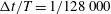
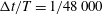
) are selected. Figure 3(a–c) shows the coarsest wall-layer resolutions over the cycle in wall units. In spectral-element discretizations, Karniadakis & Sherwin (Reference Karniadakis and Sherwin2005) suggest to resolve the first nine wall units away from the wall with at least ten collocation points. Figure 3(b) shows that this criterion is well satisfied for both cases, as
 $\unicode[STIX]{x0394}y_{w}^{+}\leqslant 0.41$
for Case C1 and
$\unicode[STIX]{x0394}y_{w}^{+}\leqslant 0.41$
for Case C1 and
 $\unicode[STIX]{x0394}y_{w}^{+}\leqslant 0.22$
for Case C2. Standard values for the streamwise and spanwise grid resolutions in recent DNS studies of wall-bounded flows are in the range
$\unicode[STIX]{x0394}y_{w}^{+}\leqslant 0.22$
for Case C2. Standard values for the streamwise and spanwise grid resolutions in recent DNS studies of wall-bounded flows are in the range
 $\unicode[STIX]{x0394}x^{+}\approx 12$
and
$\unicode[STIX]{x0394}x^{+}\approx 12$
and
 $\unicode[STIX]{x0394}z^{+}\approx 6$
, e.g. Hoyas & Jiménez (Reference Hoyas and Jiménez2006) employed
$\unicode[STIX]{x0394}z^{+}\approx 6$
, e.g. Hoyas & Jiménez (Reference Hoyas and Jiménez2006) employed
 $(12.3,0.323,6.1)$
and Lozano-Durán & Jiménez (Reference Lozano-Durán and Jiménez2014) employed
$(12.3,0.323,6.1)$
and Lozano-Durán & Jiménez (Reference Lozano-Durán and Jiménez2014) employed
 $(12.8,0.314,6.4)$
for
$(12.8,0.314,6.4)$
for
 $(\unicode[STIX]{x0394}x^{+},\unicode[STIX]{x0394}y_{w}^{+},\unicode[STIX]{x0394}z^{+})$
resolutions, respectively. Figure 3(a,c) shows that the resolutions in these directions are well within these ranges for both cases. Moreover, our streamwise resolution is finer with
$(\unicode[STIX]{x0394}x^{+},\unicode[STIX]{x0394}y_{w}^{+},\unicode[STIX]{x0394}z^{+})$
resolutions, respectively. Figure 3(a,c) shows that the resolutions in these directions are well within these ranges for both cases. Moreover, our streamwise resolution is finer with
 $\unicode[STIX]{x0394}x^{+}\leqslant 4.1$
for Case C1 and
$\unicode[STIX]{x0394}x^{+}\leqslant 4.1$
for Case C1 and
 $\unicode[STIX]{x0394}x^{+}\leqslant 2.2$
for Case C2, as we have to resolve the additional effects due to streamwise pressure gradients and the curvature of the ripple.
$\unicode[STIX]{x0394}x^{+}\leqslant 2.2$
for Case C2, as we have to resolve the additional effects due to streamwise pressure gradients and the curvature of the ripple.

Figure 3. Extremal grid spacings over a flow cycle. (a–c) Largest grid spacings on the wall in wall units.
 $\unicode[STIX]{x0394}y_{w}$
is the vertical distance of the first grid point from the ripple surface. (d,e) Largest grid spacings in free stream in Kolmogorov units (
$\unicode[STIX]{x0394}y_{w}$
is the vertical distance of the first grid point from the ripple surface. (d,e) Largest grid spacings in free stream in Kolmogorov units (
 $l_{\unicode[STIX]{x1D702}}=(\unicode[STIX]{x1D708}^{3}/\unicode[STIX]{x1D700})^{1/4}$
).
$l_{\unicode[STIX]{x1D702}}=(\unicode[STIX]{x1D708}^{3}/\unicode[STIX]{x1D700})^{1/4}$
).
 $\unicode[STIX]{x0394}l$
is the representative grid spacing in the unstructured hp–FEM mesh, cf. (2.6). (–○): Case C1; (–▫): Case C2.
$\unicode[STIX]{x0394}l$
is the representative grid spacing in the unstructured hp–FEM mesh, cf. (2.6). (–○): Case C1; (–▫): Case C2.
In free stream, the smallest eddies in the dissipation range have to be resolved. According to Kolmogorov’s first hypothesis of similarity (Kolmogorov Reference Kolmogorov1941), the local isotropic Kolmogorov microscale
 $l_{\unicode[STIX]{x1D702}}=(\unicode[STIX]{x1D708}^{3}/\unicode[STIX]{x1D700})^{1/4}$
is the length scale of the smallest eddies where
$l_{\unicode[STIX]{x1D702}}=(\unicode[STIX]{x1D708}^{3}/\unicode[STIX]{x1D700})^{1/4}$
is the length scale of the smallest eddies where
 $\unicode[STIX]{x1D700}$
is the local dissipation rate, cf. (4.4). The spectral elements are unstructured and approximately isotropic in regions
$\unicode[STIX]{x1D700}$
is the local dissipation rate, cf. (4.4). The spectral elements are unstructured and approximately isotropic in regions
 $\unicode[STIX]{x1D6FA}_{2}$
and
$\unicode[STIX]{x1D6FA}_{2}$
and
 $\unicode[STIX]{x1D6FA}_{3}$
where coherent vortices spend most of their lives. Therefore, the resolution in the
$\unicode[STIX]{x1D6FA}_{3}$
where coherent vortices spend most of their lives. Therefore, the resolution in the
 $x$
–
$x$
–
 $y$
plane is checked by comparing the local
$y$
plane is checked by comparing the local
 $l_{\unicode[STIX]{x1D702}}$
to the element length scale
$l_{\unicode[STIX]{x1D702}}$
to the element length scale
 $\unicode[STIX]{x0394}l$
(cf. (2.6)). In the spanwise direction, a constant spacing
$\unicode[STIX]{x0394}l$
(cf. (2.6)). In the spanwise direction, a constant spacing
 $\unicode[STIX]{x0394}z$
is used. The largest free-stream resolutions over the cycle are plotted in figure 3(d,e). We see that grid spacings are of the order of the Kolmogorov scales with
$\unicode[STIX]{x0394}z$
is used. The largest free-stream resolutions over the cycle are plotted in figure 3(d,e). We see that grid spacings are of the order of the Kolmogorov scales with
 $\unicode[STIX]{x0394}l/l_{\unicode[STIX]{x1D702}}\leqslant 2.8$
,
$\unicode[STIX]{x0394}l/l_{\unicode[STIX]{x1D702}}\leqslant 2.8$
,
 $\unicode[STIX]{x0394}z/l_{\unicode[STIX]{x1D702}}\leqslant 2.9$
for Case C1,
$\unicode[STIX]{x0394}z/l_{\unicode[STIX]{x1D702}}\leqslant 2.9$
for Case C1,
 $\unicode[STIX]{x0394}l/l_{\unicode[STIX]{x1D702}}\leqslant 1.26$
,and
$\unicode[STIX]{x0394}l/l_{\unicode[STIX]{x1D702}}\leqslant 1.26$
,and
 $\unicode[STIX]{x0394}z/l_{\unicode[STIX]{x1D702}}\leqslant 1.54$
. Mahesh & Moin (Reference Mahesh and Moin1998) remarks that the smallest resolved length scale in a DNS is required to be
$\unicode[STIX]{x0394}z/l_{\unicode[STIX]{x1D702}}\leqslant 1.54$
. Mahesh & Moin (Reference Mahesh and Moin1998) remarks that the smallest resolved length scale in a DNS is required to be
 $O(l_{\unicode[STIX]{x1D702}})$
, not
$O(l_{\unicode[STIX]{x1D702}})$
, not
 $l_{\unicode[STIX]{x1D702}}$
, as accurate first- and second-order statistics can be obtained when most of the dissipation is captured. In this regard, the selected spatial resolutions are sufficient for both cases, and we will show in appendix A that dissipation is also well captured.
$l_{\unicode[STIX]{x1D702}}$
, as accurate first- and second-order statistics can be obtained when most of the dissipation is captured. In this regard, the selected spatial resolutions are sufficient for both cases, and we will show in appendix A that dissipation is also well captured.
3 Phase-locked vortex kinematics
In this section, we discuss the kinematics of wave-induced flow over ripples with a special emphasis on the motion of coherent spanwise vortices. In the considered oscillatory flow, ensemble averaging is approximated using phase-locked averaging combined with spatial averaging over homogeneous direction and ripple-based averaging, e.g. for velocity,
 $$\begin{eqnarray}\langle \boldsymbol{u}\rangle (x,y,t)=\frac{1}{NM}\mathop{\sum }_{m=0}^{M-1}\mathop{\sum }_{n=0}^{N-1}\tilde{\boldsymbol{u}}(x+m\unicode[STIX]{x1D706},y,t+nT),\quad 0\leqslant x<\unicode[STIX]{x1D706},0\leqslant t<T,\end{eqnarray}$$
where
 $\tilde{\boldsymbol{u}}$
is the spatially averaged velocity over the homogeneous direction
$\tilde{\boldsymbol{u}}$
is the spatially averaged velocity over the homogeneous direction
 $z$
,
$z$
,
 $N$
is the total number of sampling periods and
$N$
is the total number of sampling periods and
 $M$
is the number of ripples in the domain. Using this averaging, Reynolds decomposition is applied to the fields of interest, e.g.
$M$
is the number of ripples in the domain. Using this averaging, Reynolds decomposition is applied to the fields of interest, e.g.
 $\boldsymbol{u}=\langle \boldsymbol{u}\rangle +\boldsymbol{u}^{\prime }$
, where
$\boldsymbol{u}=\langle \boldsymbol{u}\rangle +\boldsymbol{u}^{\prime }$
, where
 $\boldsymbol{u}^{\prime }$
is the fluctuating part of the turbulent velocity field.
$\boldsymbol{u}^{\prime }$
is the fluctuating part of the turbulent velocity field.

Figure 4. (a–h) Evolution of vorticity and velocity fields along the half-cycle for Case C1. (Left) Contours of phase-averaged spanwise vorticity
 $\langle \unicode[STIX]{x1D714}_{z}\rangle$
; (right) the phase-averaged velocity
$\langle \unicode[STIX]{x1D714}_{z}\rangle$
; (right) the phase-averaged velocity
 $\langle \boldsymbol{u}\rangle$
vectors. The values in parentheses show the normalized circulation
$\langle \boldsymbol{u}\rangle$
vectors. The values in parentheses show the normalized circulation
 $\unicode[STIX]{x1D6E4}/U_{0}\unicode[STIX]{x1D702}$
of the vortices, cf. (3.3). The thick lines show a section of the isolines
$\unicode[STIX]{x1D6E4}/U_{0}\unicode[STIX]{x1D702}$
of the vortices, cf. (3.3). The thick lines show a section of the isolines
 $\langle p\rangle$
, which are employed to separate
$\langle p\rangle$
, which are employed to separate
 $P$
- and
$P$
- and
 $S$
-vortices; (a,b)
$S$
-vortices; (a,b)
 $\langle p\rangle /\unicode[STIX]{x1D70C}U_{0}^{2}=0.2$
and (h)
$\langle p\rangle /\unicode[STIX]{x1D70C}U_{0}^{2}=0.2$
and (h)
 $\langle p\rangle /\unicode[STIX]{x1D70C}U_{0}^{2}=0.075$
.
$\langle p\rangle /\unicode[STIX]{x1D70C}U_{0}^{2}=0.075$
.
Figure 5. Evolution of vorticity and velocity fields along the half-cycle for Case C2. See figure 4 for captions.
Figures 4 and 5 show the phase-averaged spanwise vorticity
 $\langle \unicode[STIX]{x1D714}_{z}\rangle$
contours, i.e.
$\langle \unicode[STIX]{x1D714}_{z}\rangle$
contours, i.e.
 $$\begin{eqnarray}\langle \unicode[STIX]{x1D714}_{z}\rangle =\frac{\unicode[STIX]{x2202}\langle u_{y}\rangle }{\unicode[STIX]{x2202}x}-\frac{\unicode[STIX]{x2202}\langle u_{x}\rangle }{\unicode[STIX]{x2202}y},\end{eqnarray}$$
and velocity
 $\langle \boldsymbol{u}\rangle$
vectors along the half-cycle (
$\langle \boldsymbol{u}\rangle$
vectors along the half-cycle (
 $0\leqslant \unicode[STIX]{x1D703}<\unicode[STIX]{x03C0}$
) for cases C1 and C2, respectively. We will use the
$0\leqslant \unicode[STIX]{x1D703}<\unicode[STIX]{x03C0}$
) for cases C1 and C2, respectively. We will use the
 $\langle \unicode[STIX]{x1D714}_{z}\rangle$
-field to discuss the coherent-vortex kinematics. To this end, we define a coherent vortex as an enclosed region of concentrated
$\langle \unicode[STIX]{x1D714}_{z}\rangle$
-field to discuss the coherent-vortex kinematics. To this end, we define a coherent vortex as an enclosed region of concentrated
 $\langle \unicode[STIX]{x1D714}_{z}\rangle$
. Similar definitions have previously been employed in the studies of turbulent coherent structures in free-shear flows, cf. e.g. Hussain (Reference Hussain1986). The strength of a coherent vortex can be measured by its circulation, which is calculated by (Batchelor Reference Batchelor2000)
$\langle \unicode[STIX]{x1D714}_{z}\rangle$
. Similar definitions have previously been employed in the studies of turbulent coherent structures in free-shear flows, cf. e.g. Hussain (Reference Hussain1986). The strength of a coherent vortex can be measured by its circulation, which is calculated by (Batchelor Reference Batchelor2000)
 $$\begin{eqnarray}\unicode[STIX]{x1D6E4}=\oint _{C}\langle \boldsymbol{u}\rangle \boldsymbol{\cdot }\text{d}\boldsymbol{l}=\int _{A}\langle \unicode[STIX]{x1D714}_{z}\rangle \,\text{d}A,\end{eqnarray}$$
where
 $C$
is the closed curve representing the vortex boundary, and
$C$
is the closed curve representing the vortex boundary, and
 $A$
is the area of the vortex region. We have selected the contours
$A$
is the area of the vortex region. We have selected the contours
 $|\langle \unicode[STIX]{x1D714}_{z}\rangle |=0.15U_{0}/\unicode[STIX]{x1D702}$
as the boundary threshold for vortices. This value corresponds to the lowest contour level in figures 4 and 5, and it is approximately
$|\langle \unicode[STIX]{x1D714}_{z}\rangle |=0.15U_{0}/\unicode[STIX]{x1D702}$
as the boundary threshold for vortices. This value corresponds to the lowest contour level in figures 4 and 5, and it is approximately
 $2.5\,\%$
of the maximum vorticity level in the figures. The circulation of coherent vortices is presented in parentheses in figures 4 and 5. These values can be compared with the total circulation around a single ripple, which can be calculated using a line integral on a closed curve containing the ripple surface, vertical lines normal to the troughs and a horizontal line in the free stream. In our cases, the total circulation at a phase equals to
$2.5\,\%$
of the maximum vorticity level in the figures. The circulation of coherent vortices is presented in parentheses in figures 4 and 5. These values can be compared with the total circulation around a single ripple, which can be calculated using a line integral on a closed curve containing the ripple surface, vertical lines normal to the troughs and a horizontal line in the free stream. In our cases, the total circulation at a phase equals to
 $\unicode[STIX]{x1D6E4}_{R}=-u_{0}\unicode[STIX]{x1D706}=-6u_{0}\unicode[STIX]{x1D702}$
.
$\unicode[STIX]{x1D6E4}_{R}=-u_{0}\unicode[STIX]{x1D706}=-6u_{0}\unicode[STIX]{x1D702}$
.
Figure 6(a,b) further shows the vorticity distributions on the ripple surface
 $\unicode[STIX]{x1D6FA}_{\unicode[STIX]{x1D702}}$
, i.e.
$\unicode[STIX]{x1D6FA}_{\unicode[STIX]{x1D702}}$
, i.e.
 $$\begin{eqnarray}\langle \unicode[STIX]{x1D714}_{z}(\boldsymbol{x},\unicode[STIX]{x1D703})\rangle =-\frac{\unicode[STIX]{x2202}\langle \boldsymbol{u}(\boldsymbol{x},\unicode[STIX]{x1D703})\rangle }{\unicode[STIX]{x2202}\boldsymbol{x}}\boldsymbol{\cdot }\hat{\boldsymbol{n}}\quad \text{for }\boldsymbol{x}\in \unicode[STIX]{x1D6FA}_{\unicode[STIX]{x1D702}},\end{eqnarray}$$
where
 $\hat{\boldsymbol{n}}$
is the normal of the ripple surface (cf. figure 1 for its orientation). In these figures, we consider
$\hat{\boldsymbol{n}}$
is the normal of the ripple surface (cf. figure 1 for its orientation). In these figures, we consider
 $\langle \unicode[STIX]{x1D714}_{z}\rangle =0$
(thick solid lines) as the average position of the separation and reattachment points.
$\langle \unicode[STIX]{x1D714}_{z}\rangle =0$
(thick solid lines) as the average position of the separation and reattachment points.

Figure 6. Distribution of the phase-averaged spanwise vorticity
 $\langle \unicode[STIX]{x1D714}_{z}\rangle$
on the ripple surface around the cycle. The thick solid lines show
$\langle \unicode[STIX]{x1D714}_{z}\rangle$
on the ripple surface around the cycle. The thick solid lines show
 $\langle \unicode[STIX]{x1D714}_{z}\rangle =0$
. The dashed lines bound the time interval without flow separation. The dotted lines show the position of the minimum vorticity on the ripple for
$\langle \unicode[STIX]{x1D714}_{z}\rangle =0$
. The dashed lines bound the time interval without flow separation. The dotted lines show the position of the minimum vorticity on the ripple for
 $0\leqslant \unicode[STIX]{x1D703}\leqslant 40\unicode[STIX]{x03C0}/32$
. A local ripple coordinate
$0\leqslant \unicode[STIX]{x1D703}\leqslant 40\unicode[STIX]{x03C0}/32$
. A local ripple coordinate
 $x^{\prime }=(x-x_{c})/\unicode[STIX]{x1D706}$
is employed with
$x^{\prime }=(x-x_{c})/\unicode[STIX]{x1D706}$
is employed with
 $x_{c}$
being the streamwise location of the ripple crest.
$x_{c}$
being the streamwise location of the ripple crest.
We will discuss the deceleration and acceleration phases in §§ 3.1 and 3.2, respectively. In the deceleration phase between
 $0\leqslant \unicode[STIX]{x1D703}<\unicode[STIX]{x03C0}/2$
(figures 4
a–d and 5
a–d). In this stage, new vortices form and start absorbing the flow energy. Therefore, we will also denote the deceleration phase as the vortex-formation phase. In the acceleration stage in the interval
$0\leqslant \unicode[STIX]{x1D703}<\unicode[STIX]{x03C0}/2$
(figures 4
a–d and 5
a–d). In this stage, new vortices form and start absorbing the flow energy. Therefore, we will also denote the deceleration phase as the vortex-formation phase. In the acceleration stage in the interval
 $\unicode[STIX]{x03C0}/2\leqslant \unicode[STIX]{x1D703}<\unicode[STIX]{x03C0}$
(figures 4
e–h and 5
e–h), the coherent vortices travel large distances with their self-induced velocities, and produce jet-like flows. We will denote the acceleration phase as the jet ejection, or simply ejection, phase.
$\unicode[STIX]{x03C0}/2\leqslant \unicode[STIX]{x1D703}<\unicode[STIX]{x03C0}$
(figures 4
e–h and 5
e–h), the coherent vortices travel large distances with their self-induced velocities, and produce jet-like flows. We will denote the acceleration phase as the jet ejection, or simply ejection, phase.
3.1 Vortex-formation (deceleration) phase
 $(0\leqslant \unicode[STIX]{x1D703}<\unicode[STIX]{x03C0}/2)$

At the start of deceleration phase at
 $\unicode[STIX]{x1D703}=0$
, where the free-stream velocity is at its negative peak (cf. figures 4
a and 5
a), the flow separates at the crest of the ripple (
$\unicode[STIX]{x1D703}=0$
, where the free-stream velocity is at its negative peak (cf. figures 4
a and 5
a), the flow separates at the crest of the ripple (
 $x^{\prime }=0$
) and reattaches at
$x^{\prime }=0$
) and reattaches at
 $x^{\prime }\approx -0.4$
(
$x^{\prime }\approx -0.4$
(
 $x^{\prime }=(x-x_{c})/\unicode[STIX]{x1D706}$
where
$x^{\prime }=(x-x_{c})/\unicode[STIX]{x1D706}$
where
 $x_{c}$
is the streamwise location of the crest) for Case C1, cf. figure 6(a). The reattachment point in Case C2 is further downstream at the stoss side at around
$x_{c}$
is the streamwise location of the crest) for Case C1, cf. figure 6(a). The reattachment point in Case C2 is further downstream at the stoss side at around
 $x^{\prime }\approx 0.4$
, cf. figure 6(b). The positive-vorticity flux from the crest feeds the forming vortex in the lee of the ripple. We denote this vortex
$x^{\prime }\approx 0.4$
, cf. figure 6(b). The positive-vorticity flux from the crest feeds the forming vortex in the lee of the ripple. We denote this vortex
 $P^{+}$
, where
$P^{+}$
, where
 $P$
stands for primary vortex, and the superscript ‘
$P$
stands for primary vortex, and the superscript ‘
 $+$
’ indicates the positive circulation – not to be confused with the wall units superscript. Furthermore, there is a secondary vortex from previous half-cycle
$+$
’ indicates the positive circulation – not to be confused with the wall units superscript. Furthermore, there is a secondary vortex from previous half-cycle
 $(S^{+})$
with the same sense of circulation. In order to distinguish these vortices, we employ a segment of the pressure isoline
$(S^{+})$
with the same sense of circulation. In order to distinguish these vortices, we employ a segment of the pressure isoline
 $\langle p\rangle /\unicode[STIX]{x1D70C}U_{0}^{2}=0.2$
, cf. the thick solid lines in figures 4(a,b) and 5(a,b). This practical selection is based on the observation that the ejected secondary vortex quickly loses its property of being a low-pressure centre after being detached from the ripple crest. Moreover, the boundary layer beneath the
$\langle p\rangle /\unicode[STIX]{x1D70C}U_{0}^{2}=0.2$
, cf. the thick solid lines in figures 4(a,b) and 5(a,b). This practical selection is based on the observation that the ejected secondary vortex quickly loses its property of being a low-pressure centre after being detached from the ripple crest. Moreover, the boundary layer beneath the
 $S^{+}$
-vortex contains the same sign of vorticity with the vortex. In order to differentiate the boundary layer and vortex regions, we exclude the wall layer of
$S^{+}$
-vortex contains the same sign of vorticity with the vortex. In order to differentiate the boundary layer and vortex regions, we exclude the wall layer of
 $\unicode[STIX]{x0394}y=2\unicode[STIX]{x1D6FF}_{s}$
thickness from the circulation field of the
$\unicode[STIX]{x0394}y=2\unicode[STIX]{x1D6FF}_{s}$
thickness from the circulation field of the
 $S^{+}$
-vortex. At
$S^{+}$
-vortex. At
 $\unicode[STIX]{x1D703}=0$
, there is another primary vortex,
$\unicode[STIX]{x1D703}=0$
, there is another primary vortex,
 $P^{-}$
, moving to the west above the ripple crest. It has formed in the previous half-cycle on the eastern side of the eastern neighbour, hence has a negative circulation. This residual vortex has around
$P^{-}$
, moving to the west above the ripple crest. It has formed in the previous half-cycle on the eastern side of the eastern neighbour, hence has a negative circulation. This residual vortex has around
 $25\,\%$
and
$25\,\%$
and
 $33\,\%$
circulation of
$33\,\%$
circulation of
 $P^{+}$
-vortices in Cases C1 and C2, respectively. This suggests a small but non-negligible flow interference between neighbouring ripples.
$P^{+}$
-vortices in Cases C1 and C2, respectively. This suggests a small but non-negligible flow interference between neighbouring ripples.

Figure 7. Formation of the secondary spanwise vortex
 $S^{-}$
via flow separation induced by the adverse pressure gradient in the primary vortex
$S^{-}$
via flow separation induced by the adverse pressure gradient in the primary vortex
 $P^{+}$
at
$P^{+}$
at
 $\unicode[STIX]{x1D703}=8\unicode[STIX]{x03C0}/32$
. Shaded contours show
$\unicode[STIX]{x1D703}=8\unicode[STIX]{x03C0}/32$
. Shaded contours show
 $\langle p\rangle /\unicode[STIX]{x1D70C}U_{0}^{2}$
. The thick contour lines are
$\langle p\rangle /\unicode[STIX]{x1D70C}U_{0}^{2}$
. The thick contour lines are
 $\unicode[STIX]{x1D6EC}=1/2(\unicode[STIX]{x1D6FA}_{ij}\unicode[STIX]{x1D6FA}_{ij}-\unicode[STIX]{x1D61A}_{ij}\unicode[STIX]{x1D61A}_{ij})=0$
. Blue contours show
$\unicode[STIX]{x1D6EC}=1/2(\unicode[STIX]{x1D6FA}_{ij}\unicode[STIX]{x1D6FA}_{ij}-\unicode[STIX]{x1D61A}_{ij}\unicode[STIX]{x1D61A}_{ij})=0$
. Blue contours show
 $\langle \unicode[STIX]{x1D714}_{z}\rangle /(U_{0}/\unicode[STIX]{x1D702})=|0.15|$
indicating the coherent-vortex boundaries.
$\langle \unicode[STIX]{x1D714}_{z}\rangle /(U_{0}/\unicode[STIX]{x1D702})=|0.15|$
indicating the coherent-vortex boundaries.
We further see at
 $\unicode[STIX]{x1D703}=0$
that
$\unicode[STIX]{x1D703}=0$
that
 $P^{+}$
-vortex induces a thin boundary layer on the wall with reverse circulation, cf. the negative vorticity contours at the lee side (
$P^{+}$
-vortex induces a thin boundary layer on the wall with reverse circulation, cf. the negative vorticity contours at the lee side (
 $x^{\prime }<0$
) in figure 6(a,b). While the vorticity flux at the crest keeps increasing the circulation of
$x^{\prime }<0$
) in figure 6(a,b). While the vorticity flux at the crest keeps increasing the circulation of
 $P^{+}$
, the reverse flow becomes also stronger, cf.
$P^{+}$
, the reverse flow becomes also stronger, cf.
 $S^{-}$
in figures 4(b,c) and 5(b,c). Furthermore, the low-pressure zone in the
$S^{-}$
in figures 4(b,c) and 5(b,c). Furthermore, the low-pressure zone in the
 $P^{+}$
-vortex intensifies, and a strong adverse pressure gradient is created along the ripple surface at the lee side. This is shown in figure 7 for both cases at phase
$P^{+}$
-vortex intensifies, and a strong adverse pressure gradient is created along the ripple surface at the lee side. This is shown in figure 7 for both cases at phase
 $\unicode[STIX]{x1D703}=8\unicode[STIX]{x03C0}/32$
. The adverse pressure gradient along the wall yields a secondary flow separation within the vortex-induced boundary layer, cf. positive-vorticity islands at the lee side (
$\unicode[STIX]{x1D703}=8\unicode[STIX]{x03C0}/32$
. The adverse pressure gradient along the wall yields a secondary flow separation within the vortex-induced boundary layer, cf. positive-vorticity islands at the lee side (
 $x^{\prime }<0$
) in
$x^{\prime }<0$
) in
 $2\unicode[STIX]{x03C0}/32\leqslant \unicode[STIX]{x1D703}\leqslant 9\unicode[STIX]{x03C0}/32$
for C1 and in
$2\unicode[STIX]{x03C0}/32\leqslant \unicode[STIX]{x1D703}\leqslant 9\unicode[STIX]{x03C0}/32$
for C1 and in
 $4\unicode[STIX]{x03C0}/32\leqslant \unicode[STIX]{x1D703}\leqslant 12\unicode[STIX]{x03C0}/32$
for C2 in figure 6(a,b). Following the separation,
$4\unicode[STIX]{x03C0}/32\leqslant \unicode[STIX]{x1D703}\leqslant 12\unicode[STIX]{x03C0}/32$
for C2 in figure 6(a,b). Following the separation,
 $S^{-}$
rolls into a secondary separation bubble. Figure 7 demonstrates this using the Okubo–Weiss parameter
$S^{-}$
rolls into a secondary separation bubble. Figure 7 demonstrates this using the Okubo–Weiss parameter
 $\unicode[STIX]{x1D6EC}=1/2(\unicode[STIX]{x1D6FA}_{ij}\unicode[STIX]{x1D6FA}_{ij}-\unicode[STIX]{x1D61A}_{ij}\unicode[STIX]{x1D61A}_{ij})$
, where
$\unicode[STIX]{x1D6EC}=1/2(\unicode[STIX]{x1D6FA}_{ij}\unicode[STIX]{x1D6FA}_{ij}-\unicode[STIX]{x1D61A}_{ij}\unicode[STIX]{x1D61A}_{ij})$
, where
 $\unicode[STIX]{x1D6FA}_{ij}=1/2(\unicode[STIX]{x2202}\langle u_{i}\rangle /\unicode[STIX]{x2202}x_{j}-\unicode[STIX]{x2202}\langle u_{j}\rangle /\unicode[STIX]{x2202}x_{i})$
is the phase-averaged rate of rotation tensor,
$\unicode[STIX]{x1D6FA}_{ij}=1/2(\unicode[STIX]{x2202}\langle u_{i}\rangle /\unicode[STIX]{x2202}x_{j}-\unicode[STIX]{x2202}\langle u_{j}\rangle /\unicode[STIX]{x2202}x_{i})$
is the phase-averaged rate of rotation tensor,
 $\unicode[STIX]{x1D6FA}_{ij}\unicode[STIX]{x1D6FA}_{ij}=1/2\langle \unicode[STIX]{x1D714}_{z}\rangle ^{2}$
in two dimensions and
$\unicode[STIX]{x1D6FA}_{ij}\unicode[STIX]{x1D6FA}_{ij}=1/2\langle \unicode[STIX]{x1D714}_{z}\rangle ^{2}$
in two dimensions and
 $$\begin{eqnarray}\unicode[STIX]{x1D61A}_{ij}=\frac{1}{2}\left(\frac{\unicode[STIX]{x2202}\langle u_{i}\rangle }{\unicode[STIX]{x2202}x_{j}}+\frac{\unicode[STIX]{x2202}\langle u_{j}\rangle }{\unicode[STIX]{x2202}x_{i}}\right)\end{eqnarray}$$
is the phase-averaged rate of strain tensor. Positive values of
 $\unicode[STIX]{x1D6EC}$
identify vortex cores where the vorticity prevails over strain (Okubo Reference Okubo1970; Weiss Reference Weiss1991). To this end, the isoline of
$\unicode[STIX]{x1D6EC}$
identify vortex cores where the vorticity prevails over strain (Okubo Reference Okubo1970; Weiss Reference Weiss1991). To this end, the isoline of
 $\unicode[STIX]{x1D6EC}=0$
shows the development of secondary separation bubble in
$\unicode[STIX]{x1D6EC}=0$
shows the development of secondary separation bubble in
 $S^{-}$
for both cases in figure 7. General properties of secondary vortex development due to vortex-induced separation are discussed in Doligalski, Smith & Walker (Reference Doligalski, Smith and Walker1994). In the case of vortex ripples, the phenomenon has been documented previously by Blondeaux & Vittori (Reference Blondeaux and Vittori1991) in a two-dimensional setting. The coherent secondary vortex is not captured in studies with discrete vortex models, e.g. cf. Longuet-Higgins (Reference Longuet-Higgins1981), and sometimes not captured in experiments either, cf. e.g. Earnshaw & Greated (Reference Earnshaw and Greated1998) and Fredsøe et al. (Reference Fredsøe, Andersen and Sumer1999).
$S^{-}$
for both cases in figure 7. General properties of secondary vortex development due to vortex-induced separation are discussed in Doligalski, Smith & Walker (Reference Doligalski, Smith and Walker1994). In the case of vortex ripples, the phenomenon has been documented previously by Blondeaux & Vittori (Reference Blondeaux and Vittori1991) in a two-dimensional setting. The coherent secondary vortex is not captured in studies with discrete vortex models, e.g. cf. Longuet-Higgins (Reference Longuet-Higgins1981), and sometimes not captured in experiments either, cf. e.g. Earnshaw & Greated (Reference Earnshaw and Greated1998) and Fredsøe et al. (Reference Fredsøe, Andersen and Sumer1999).
The coherent spanwise vortices are highly turbulent structures. Therefore, the amount of spanwise vorticity shed from the crest is considerably higher than that absorbed in the
 $P^{+}$
-vortex. This can be shown by comparing the shed and absorbed circulations in the temporal range with prominent flow separation, i.e.
$P^{+}$
-vortex. This can be shown by comparing the shed and absorbed circulations in the temporal range with prominent flow separation, i.e.
 $0\leqslant \unicode[STIX]{x1D703}<12\unicode[STIX]{x03C0}/32$
. To this end, the total positive-vorticity flux across the boundary layer above the crest, which is located at
$0\leqslant \unicode[STIX]{x1D703}<12\unicode[STIX]{x03C0}/32$
. To this end, the total positive-vorticity flux across the boundary layer above the crest, which is located at
 $(x_{c},y_{c}=y_{\unicode[STIX]{x1D702}}(x_{c}))$
, can be calculated using
$(x_{c},y_{c}=y_{\unicode[STIX]{x1D702}}(x_{c}))$
, can be calculated using
 $$\begin{eqnarray}\dot{\unicode[STIX]{x1D6E4}}_{c}=\int _{y_{\unicode[STIX]{x1D702}}(x_{c})}^{y_{\unicode[STIX]{x1D6FF}}}\langle u_{x}(x_{c},y)\rangle \langle \unicode[STIX]{x1D714}_{z}(x_{c},y)\rangle \,\text{d}y,\end{eqnarray}$$
where
 $y_{\unicode[STIX]{x1D6FF}}$
is the vertical coordinate of the peak streamwise velocity. Consequently, the total shed positive vorticity from the crest in a range
$y_{\unicode[STIX]{x1D6FF}}$
is the vertical coordinate of the peak streamwise velocity. Consequently, the total shed positive vorticity from the crest in a range
 $\unicode[STIX]{x1D703}_{i}\leqslant \unicode[STIX]{x1D703}\leqslant \unicode[STIX]{x1D703}_{f}$
is given by
$\unicode[STIX]{x1D703}_{i}\leqslant \unicode[STIX]{x1D703}\leqslant \unicode[STIX]{x1D703}_{f}$
is given by
 $$\begin{eqnarray}\unicode[STIX]{x0394}\unicode[STIX]{x1D6E4}_{c}(\unicode[STIX]{x1D703}_{i},\unicode[STIX]{x1D703}_{f})=\int _{t=\unicode[STIX]{x1D703}_{i}/\unicode[STIX]{x1D714}}^{t=\unicode[STIX]{x1D703}_{f}/\unicode[STIX]{x1D714}}\dot{\unicode[STIX]{x1D6E4}}_{c}\,\text{d}t.\end{eqnarray}$$
Figure 8 compares the net shed positive vorticity
 $\unicode[STIX]{x0394}\unicode[STIX]{x1D6E4}_{c}(0,\unicode[STIX]{x1D703})$
with the net absorbed circulation in
$\unicode[STIX]{x0394}\unicode[STIX]{x1D6E4}_{c}(0,\unicode[STIX]{x1D703})$
with the net absorbed circulation in
 $P^{+}$
, i.e.
$P^{+}$
, i.e.
 $\unicode[STIX]{x0394}\unicode[STIX]{x1D6E4}_{P+}=\unicode[STIX]{x1D6E4}_{P+}(\unicode[STIX]{x1D703})-\unicode[STIX]{x1D6E4}_{P+}(0)$
. We see that
$\unicode[STIX]{x0394}\unicode[STIX]{x1D6E4}_{P+}=\unicode[STIX]{x1D6E4}_{P+}(\unicode[STIX]{x1D703})-\unicode[STIX]{x1D6E4}_{P+}(0)$
. We see that
 $P^{+}$
cannot keep most of the shed circulation, and the gap
$P^{+}$
cannot keep most of the shed circulation, and the gap
 $\unicode[STIX]{x0394}\unicode[STIX]{x1D6E4}_{c}-\unicode[STIX]{x0394}\unicode[STIX]{x1D6E4}_{P+}$
grows with time. In particular,
$\unicode[STIX]{x0394}\unicode[STIX]{x1D6E4}_{c}-\unicode[STIX]{x0394}\unicode[STIX]{x1D6E4}_{P+}$
grows with time. In particular,
 $\unicode[STIX]{x0394}\unicode[STIX]{x1D6E4}_{P+}$
starts to decay for both cases after
$\unicode[STIX]{x0394}\unicode[STIX]{x1D6E4}_{P+}$
starts to decay for both cases after
 $\unicode[STIX]{x1D703}>6\unicode[STIX]{x03C0}/32$
showing that the loss of circulation due to turbulent diffusion dominates over the gain due to positive-vorticity flux from the crest. The shed circulation is higher in Case C1 but the overall absorbed vorticity in the primary vortex is less for this case. This suggests a more active turbulent dynamics in
$\unicode[STIX]{x1D703}>6\unicode[STIX]{x03C0}/32$
showing that the loss of circulation due to turbulent diffusion dominates over the gain due to positive-vorticity flux from the crest. The shed circulation is higher in Case C1 but the overall absorbed vorticity in the primary vortex is less for this case. This suggests a more active turbulent dynamics in
 $P^{+}$
for C1. The turbulence properties of vortices will be discussed in § 5.
$P^{+}$
for C1. The turbulence properties of vortices will be discussed in § 5.

Figure 8. Comparison between the net shed circulation at the crest (
 $\unicode[STIX]{x0394}\unicode[STIX]{x1D6E4}_{c}(0,\unicode[STIX]{x1D703})$
, cf. (3.7)) and the absorbed circulation (
$\unicode[STIX]{x0394}\unicode[STIX]{x1D6E4}_{c}(0,\unicode[STIX]{x1D703})$
, cf. (3.7)) and the absorbed circulation (
 $\unicode[STIX]{x0394}\unicode[STIX]{x1D6E4}_{P+}=\unicode[STIX]{x1D6E4}_{P+}(\unicode[STIX]{x1D703})-\unicode[STIX]{x1D6E4}_{P+}(0)$
) in the primary vortex
$\unicode[STIX]{x0394}\unicode[STIX]{x1D6E4}_{P+}=\unicode[STIX]{x1D6E4}_{P+}(\unicode[STIX]{x1D703})-\unicode[STIX]{x1D6E4}_{P+}(0)$
) in the primary vortex
 $P^{+}$
during its formation. Circulations are normalized by
$P^{+}$
during its formation. Circulations are normalized by
 $U_{0}\unicode[STIX]{x1D702}$
.
$U_{0}\unicode[STIX]{x1D702}$
.
We see in figures 4(c,d) and 5(c,d) that the
 $P^{+}$
vortex grows and spreads vertically when the free-stream velocity further decelerates. Moreover, the passing residual vortex
$P^{+}$
vortex grows and spreads vertically when the free-stream velocity further decelerates. Moreover, the passing residual vortex
 $P^{-}$
pushes
$P^{-}$
pushes
 $P^{+}$
slightly away from the crest, and moves the reattachment point of
$P^{+}$
slightly away from the crest, and moves the reattachment point of
 $P^{+}$
further towards west to the stoss region, cf.
$P^{+}$
further towards west to the stoss region, cf.
 $\langle \unicode[STIX]{x1D714}_{z}\rangle =0$
contours in figure 6. The motion of
$\langle \unicode[STIX]{x1D714}_{z}\rangle =0$
contours in figure 6. The motion of
 $P^{+}$
during its formation can also be tracked by the location of the most-intense vorticity on the ripple surface, cf. the dotted lines in figure 6. In this regard,
$P^{+}$
during its formation can also be tracked by the location of the most-intense vorticity on the ripple surface, cf. the dotted lines in figure 6. In this regard,
 $P^{+}$
moves towards the trough of the ripple until
$P^{+}$
moves towards the trough of the ripple until
 $\unicode[STIX]{x1D703}=12\unicode[STIX]{x03C0}/32$
, and then heads back to the crest, when its self-induction dominates over the weakening free-stream velocity. The boundary layer at the stoss side stops separating at
$\unicode[STIX]{x1D703}=12\unicode[STIX]{x03C0}/32$
, and then heads back to the crest, when its self-induction dominates over the weakening free-stream velocity. The boundary layer at the stoss side stops separating at
 $\unicode[STIX]{x1D703}=14\unicode[STIX]{x03C0}/32$
, and a reverse flow to the east follows subsequently on the whole ripple until around
$\unicode[STIX]{x1D703}=14\unicode[STIX]{x03C0}/32$
, and a reverse flow to the east follows subsequently on the whole ripple until around
 $\unicode[STIX]{x1D703}=20\unicode[STIX]{x03C0}/32$
. This regime without flow separation is indicated with dashed lines in figure 6.
$\unicode[STIX]{x1D703}=20\unicode[STIX]{x03C0}/32$
. This regime without flow separation is indicated with dashed lines in figure 6.
3.2 Jet-ejection (acceleration) phase
$(\unicode[STIX]{x03C0}/2\leqslant \unicode[STIX]{x1D703}<\unicode[STIX]{x03C0})$

When the free-stream velocity vanishes at
 $\unicode[STIX]{x1D703}=16\unicode[STIX]{x03C0}/32$
, the
$\unicode[STIX]{x1D703}=16\unicode[STIX]{x03C0}/32$
, the
 $P^{+}$
–
$P^{+}$
–
 $S^{-}$
vortex dipole is about to eject itself from the crest, cf. figures 4(e) and 5(e). The total circulation vanishes for this phase, i.e.
$S^{-}$
vortex dipole is about to eject itself from the crest, cf. figures 4(e) and 5(e). The total circulation vanishes for this phase, i.e.
 $\unicode[STIX]{x1D6E4}_{R}=0$
, as the free-stream velocity
$\unicode[STIX]{x1D6E4}_{R}=0$
, as the free-stream velocity
 $u_{0}$
vanishes. Therefore, the circulation contained in the near-wall layer is
$u_{0}$
vanishes. Therefore, the circulation contained in the near-wall layer is
 $\unicode[STIX]{x1D6E4}_{\unicode[STIX]{x1D708}}=-\unicode[STIX]{x1D6E4}_{P+}-\unicode[STIX]{x1D6E4}_{P-}-\unicode[STIX]{x1D6E4}_{S-}=-1.1U_{0}\unicode[STIX]{x1D702}$
for Case C1, and
$\unicode[STIX]{x1D6E4}_{\unicode[STIX]{x1D708}}=-\unicode[STIX]{x1D6E4}_{P+}-\unicode[STIX]{x1D6E4}_{P-}-\unicode[STIX]{x1D6E4}_{S-}=-1.1U_{0}\unicode[STIX]{x1D702}$
for Case C1, and
 $\unicode[STIX]{x1D6E4}_{\unicode[STIX]{x1D708}}=-0.9U_{0}\unicode[STIX]{x1D702}$
for C2. These negative values indicate the phase difference between the free stream and the wall shear.
$\unicode[STIX]{x1D6E4}_{\unicode[STIX]{x1D708}}=-0.9U_{0}\unicode[STIX]{x1D702}$
for C2. These negative values indicate the phase difference between the free stream and the wall shear.
We have discussed in § 3.1 that
 $P^{+}$
changes its convection direction ahead of the free-stream flow reversal at
$P^{+}$
changes its convection direction ahead of the free-stream flow reversal at
 $\unicode[STIX]{x1D703}=14\unicode[STIX]{x03C0}/32$
, and moves towards the crest with its self-induced velocity.
$\unicode[STIX]{x1D703}=14\unicode[STIX]{x03C0}/32$
, and moves towards the crest with its self-induced velocity.
 $P^{+}$
is stretched along an axis roughly parallel to the ripple slope during this process, and deforms into an elliptic geometry. The velocity fields in figures 4(e) and 5(e) further show that the self-induced motion produces a wall jet. This wall jet induces high shear on the wall at the footprint of the vortex, cf. encircled regions with red lines in figure 6. Further in the cycle
$P^{+}$
is stretched along an axis roughly parallel to the ripple slope during this process, and deforms into an elliptic geometry. The velocity fields in figures 4(e) and 5(e) further show that the self-induced motion produces a wall jet. This wall jet induces high shear on the wall at the footprint of the vortex, cf. encircled regions with red lines in figure 6. Further in the cycle
 $\unicode[STIX]{x1D703}=20\unicode[STIX]{x03C0}/32$
, the
$\unicode[STIX]{x1D703}=20\unicode[STIX]{x03C0}/32$
, the
 $P^{+}$
–
$P^{+}$
–
 $S^{-}$
vortex dipole ejects itself over the ripple, cf.
$S^{-}$
vortex dipole ejects itself over the ripple, cf.
 $\langle \boldsymbol{u}\rangle$
vectors in figures 4(f) and 5(f). The resulting jet is very strong with a peak velocity magnitude of approximately
$\langle \boldsymbol{u}\rangle$
vectors in figures 4(f) and 5(f). The resulting jet is very strong with a peak velocity magnitude of approximately
 $2U_{0}$
. Due to this strong jet, the maximum values in the local wall vorticity, and analogously in the local wall shear stress (cf. § 5.3 for details), are observed during the ejection process. The free jet resulting from the ejection is inclined with an angle approximately parallel to the ripple slope. While detaching from the crest, the jet and the trajectory of the vortex pair become less inclined, cf. figures 4(g) and 5(g). We note that the ejection angle is steeper in Case C2. The size and the orientation of the
$2U_{0}$
. Due to this strong jet, the maximum values in the local wall vorticity, and analogously in the local wall shear stress (cf. § 5.3 for details), are observed during the ejection process. The free jet resulting from the ejection is inclined with an angle approximately parallel to the ripple slope. While detaching from the crest, the jet and the trajectory of the vortex pair become less inclined, cf. figures 4(g) and 5(g). We note that the ejection angle is steeper in Case C2. The size and the orientation of the
 $S^{-}$
vortex appear to lead to this Reynolds number effect. The
$S^{-}$
vortex appear to lead to this Reynolds number effect. The
 $S^{-}$
vortex occupies significantly more space in C2 compared to the one in C1 due to larger boundary-layer thickness, and is more detached from the wall, cf. figure 7(a,b). Consequently, the induced velocities by the
$S^{-}$
vortex occupies significantly more space in C2 compared to the one in C1 due to larger boundary-layer thickness, and is more detached from the wall, cf. figure 7(a,b). Consequently, the induced velocities by the
 $P^{+}$
–
$P^{+}$
–
 $S^{-}$
pair are more inclined in C2, leading to a steeper ejection angle. The ejection angle has important consequences on the turbulent dynamics, which will be discussed in § 5.
$S^{-}$
pair are more inclined in C2, leading to a steeper ejection angle. The ejection angle has important consequences on the turbulent dynamics, which will be discussed in § 5.
When the vortex pair completely detaches from the crest, a new primary vortex forms at its trail, cf.
 $P^{-}$
vortices in figures 4(h) and 5(h). The detached vortices travel to the east in an approximately horizontal trajectory. In this process,
$P^{-}$
vortices in figures 4(h) and 5(h). The detached vortices travel to the east in an approximately horizontal trajectory. In this process,
 $S^{-}$
loses its circulation at a higher rate than
$S^{-}$
loses its circulation at a higher rate than
 $P^{+}$
due to interactions with the wall. This effect is less pronounced in C2, i.e.
$P^{+}$
due to interactions with the wall. This effect is less pronounced in C2, i.e.
 $\unicode[STIX]{x1D6E4}_{S-}=-1.9$
in C2, whereas
$\unicode[STIX]{x1D6E4}_{S-}=-1.9$
in C2, whereas
 $\unicode[STIX]{x1D6E4}_{S-}=-1.1$
in C1. This is due to steeper ejection angle leading a higher altitude vortex trajectory in C2, which limits the wall interference.
$\unicode[STIX]{x1D6E4}_{S-}=-1.1$
in C1. This is due to steeper ejection angle leading a higher altitude vortex trajectory in C2, which limits the wall interference.
4 Space- and time-averaged turbulence statistics
To give a global picture, we will analyse now spatially or temporally averaged fields. The main emphasis will be on the budget terms of turbulent kinetic energy (TKE)
 $k=\langle u_{i}^{\prime }u_{i}^{\prime }\rangle /2$
. The transport equation for TKE reads as follows:
$k=\langle u_{i}^{\prime }u_{i}^{\prime }\rangle /2$
. The transport equation for TKE reads as follows:
 $$\begin{eqnarray}\frac{\unicode[STIX]{x2202}k}{\unicode[STIX]{x2202}t}+\frac{\unicode[STIX]{x2202}(\langle u_{i}\rangle k+{\mathcal{T}}_{i})}{\unicode[STIX]{x2202}x_{i}}={\mathcal{P}}-\unicode[STIX]{x1D700},\end{eqnarray}$$
where
 $$\begin{eqnarray}{\mathcal{T}}_{i}={\textstyle \frac{1}{2}}\langle u_{i}^{\prime }u_{j}^{\prime }u_{j}^{\prime }\rangle +\langle u_{i}^{\prime }p^{\prime }\rangle /\unicode[STIX]{x1D70C}-2\unicode[STIX]{x1D708}\langle u_{j}^{\prime }\unicode[STIX]{x1D634}_{ij}^{\prime }\rangle\end{eqnarray}$$
contains the turbulent transport terms,
 $$\begin{eqnarray}{\mathcal{P}}=-\langle u_{i}^{\prime }u_{j}^{\prime }\rangle \frac{\unicode[STIX]{x2202}\langle u_{i}\rangle }{\unicode[STIX]{x2202}x_{j}}\end{eqnarray}$$
is the turbulent-production term, and
 $$\begin{eqnarray}\unicode[STIX]{x1D700}=2\unicode[STIX]{x1D708}\langle \unicode[STIX]{x1D634}_{ij}^{\prime }\unicode[STIX]{x1D634}_{ij}^{\prime }\rangle\end{eqnarray}$$
is the turbulent dissipation term. In (4.2) and (4.4),
 $\unicode[STIX]{x1D634}_{ij}^{\prime }$
is the fluctuating rate of strain:
$\unicode[STIX]{x1D634}_{ij}^{\prime }$
is the fluctuating rate of strain:
 $$\begin{eqnarray}\unicode[STIX]{x1D634}_{ij}^{\prime }=\frac{1}{2}\left(\frac{\unicode[STIX]{x2202}u_{i}^{\prime }}{\unicode[STIX]{x2202}x_{j}}+\frac{\unicode[STIX]{x2202}u_{j}^{\prime }}{\unicode[STIX]{x2202}x_{i}}\right).\end{eqnarray}$$
We start with the analysis of global TKE-budget. The global TKE-budget for a ripple can be obtained by spatially integrating individual terms in a periodic two-dimensional domain occupying the computational region between a ripple and the top boundary, i.e.
 ${\mathcal{V}}:=[0,\unicode[STIX]{x1D706}]\times [y_{\unicode[STIX]{x1D702}},L_{y}=1.5\unicode[STIX]{x1D706}]$
. As a result of this integration, the divergence terms on the left-hand side of (4.1) vanish, i.e.
${\mathcal{V}}:=[0,\unicode[STIX]{x1D706}]\times [y_{\unicode[STIX]{x1D702}},L_{y}=1.5\unicode[STIX]{x1D706}]$
. As a result of this integration, the divergence terms on the left-hand side of (4.1) vanish, i.e.
 $$\begin{eqnarray}\int _{{\mathcal{V}}}\frac{\unicode[STIX]{x2202}(\langle u_{i}\rangle k+{\mathcal{T}}_{i})}{\unicode[STIX]{x2202}x_{i}}\,\text{d}x\,\text{d}y=\int _{{\mathcal{S}}}n_{i}(\langle u_{i}\rangle k+{\mathcal{T}}_{i})\,\text{d}x\,\text{d}y=0,\end{eqnarray}$$
as velocity fluctuations vanish on the top boundary and the ripple wall, and the contributions on the periodic boundaries cancel out. Consequently, the local balance in (4.1) is transformed into the following simplified global form
 $$\begin{eqnarray}\frac{\text{d}k_{{\mathcal{V}}}}{\text{d}t}={\mathcal{P}}_{{\mathcal{V}}}-\unicode[STIX]{x1D700}_{{\mathcal{V}}},\end{eqnarray}$$
where
 $k_{{\mathcal{V}}}=\int _{{\mathcal{V}}}k\,\text{d}x\,\text{d}y$
,
$k_{{\mathcal{V}}}=\int _{{\mathcal{V}}}k\,\text{d}x\,\text{d}y$
,
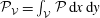 ${\mathcal{P}}_{{\mathcal{V}}}=\int _{{\mathcal{V}}}{\mathcal{P}}\,\text{d}x\,\text{d}y$
and
${\mathcal{P}}_{{\mathcal{V}}}=\int _{{\mathcal{V}}}{\mathcal{P}}\,\text{d}x\,\text{d}y$
and
 $\unicode[STIX]{x1D700}_{{\mathcal{V}}}=\int _{{\mathcal{V}}}\unicode[STIX]{x1D700}\,\text{d}x\,\text{d}y$
are global turbulent kinetic energy, production and dissipation, respectively, and are scalar functions of time.
$\unicode[STIX]{x1D700}_{{\mathcal{V}}}=\int _{{\mathcal{V}}}\unicode[STIX]{x1D700}\,\text{d}x\,\text{d}y$
are global turbulent kinetic energy, production and dissipation, respectively, and are scalar functions of time.
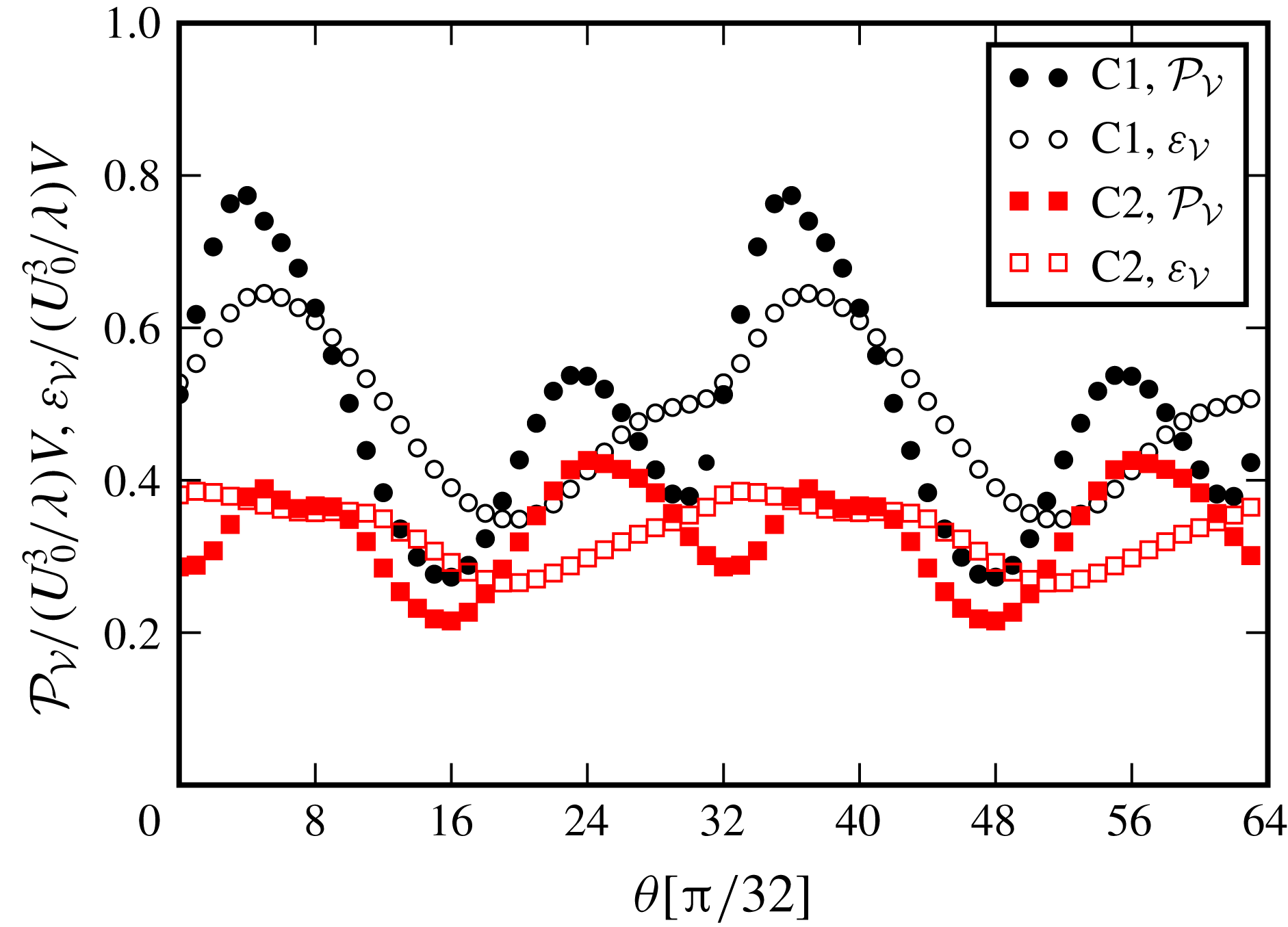
Figure 9. Evolution of global TKE production
 ${\mathcal{P}}_{{\mathcal{V}}}$
and dissipation
${\mathcal{P}}_{{\mathcal{V}}}$
and dissipation
 $\unicode[STIX]{x1D700}_{{\mathcal{V}}}$
along the cycle, cf. (4.7). For normalization we employed the area
$\unicode[STIX]{x1D700}_{{\mathcal{V}}}$
along the cycle, cf. (4.7). For normalization we employed the area
 $V=\unicode[STIX]{x1D706}\unicode[STIX]{x1D702}$
.
$V=\unicode[STIX]{x1D706}\unicode[STIX]{x1D702}$
.
Figure 9 shows the intra-period variations of
 ${\mathcal{P}}_{{\mathcal{V}}}$
and
${\mathcal{P}}_{{\mathcal{V}}}$
and
 $\unicode[STIX]{x1D700}_{{\mathcal{V}}}$
for both cases. We see two production peaks in a half-cycle, one at approximately
$\unicode[STIX]{x1D700}_{{\mathcal{V}}}$
for both cases. We see two production peaks in a half-cycle, one at approximately
 $\unicode[STIX]{x1D703}=4\unicode[STIX]{x03C0}/32$
and another at
$\unicode[STIX]{x1D703}=4\unicode[STIX]{x03C0}/32$
and another at
 $\unicode[STIX]{x1D703}=24\unicode[STIX]{x03C0}/32$
. The first peak (
$\unicode[STIX]{x1D703}=24\unicode[STIX]{x03C0}/32$
. The first peak (
 ${\mathcal{P}}_{max}^{1}$
) is roughly at the beginning of the vortex-formation stage, when the free-stream velocity is strong, and the circulation of
${\mathcal{P}}_{max}^{1}$
) is roughly at the beginning of the vortex-formation stage, when the free-stream velocity is strong, and the circulation of
 $P^{+}$
-vortex starts to saturate. The second peak (
$P^{+}$
-vortex starts to saturate. The second peak (
 ${\mathcal{P}}_{max}^{2}$
) is in the ejection phase, and corresponds to the phase when the primary vortex, along with the secondary vortex, is washed over from the ripple (cf. figures 4
g and 5
g).
${\mathcal{P}}_{max}^{2}$
) is in the ejection phase, and corresponds to the phase when the primary vortex, along with the secondary vortex, is washed over from the ripple (cf. figures 4
g and 5
g).
There is a Reynolds number effect on the production peaks, especially for
 ${\mathcal{P}}_{max}^{1}$
. The value of
${\mathcal{P}}_{max}^{1}$
. The value of
 ${\mathcal{P}}_{max}^{1}$
in Case C1 is approximately double that of Case C2. The difference in
${\mathcal{P}}_{max}^{1}$
in Case C1 is approximately double that of Case C2. The difference in
 ${\mathcal{P}}_{max}^{2}$
remains approximately
${\mathcal{P}}_{max}^{2}$
remains approximately
 $20\,\%$
. Moreover, the two production peaks in Case C2 are of similar magnitude, where
$20\,\%$
. Moreover, the two production peaks in Case C2 are of similar magnitude, where
 ${\mathcal{P}}_{max}^{1}$
clearly dominates in Case C1. Furthermore, the vortex formation stage dominates the overall
${\mathcal{P}}_{max}^{1}$
clearly dominates in Case C1. Furthermore, the vortex formation stage dominates the overall
 $k$
-production in Case C1, where both vortex formation and ejection stages make similar contributions to
$k$
-production in Case C1, where both vortex formation and ejection stages make similar contributions to
 $k$
in Case C2.
$k$
in Case C2.
We consider now time-averaged fields for a preliminary analysis of spatial distributions. Time averaging is defined as follows, e.g. for
 $k$
,
$k$
,
 $$\begin{eqnarray}\overline{k}(x,y)=\frac{1}{T}\int _{0}^{T}k(x,y,t)\,\text{d}t.\end{eqnarray}$$
Figure 10 shows the time-averaged TKE
 $\overline{k}$
, production
$\overline{k}$
, production
 $\overline{{\mathcal{P}}}$
and dissipation
$\overline{{\mathcal{P}}}$
and dissipation
 $\overline{\unicode[STIX]{x1D700}}$
for both cases. In addition to TKE-budget terms, we also consider the time-averaged fluctuating enstrophy
$\overline{\unicode[STIX]{x1D700}}$
for both cases. In addition to TKE-budget terms, we also consider the time-averaged fluctuating enstrophy
 $\overline{{\mathcal{E}}}=\overline{\langle \unicode[STIX]{x1D714}_{i}^{\prime }\unicode[STIX]{x1D714}_{i}^{\prime }\rangle }/2$
. All fields are normalized with their respective peak value, hence the contours vary between
$\overline{{\mathcal{E}}}=\overline{\langle \unicode[STIX]{x1D714}_{i}^{\prime }\unicode[STIX]{x1D714}_{i}^{\prime }\rangle }/2$
. All fields are normalized with their respective peak value, hence the contours vary between
 $[0,1]$
.
$[0,1]$
.
Figure 10(a) shows that
 $\overline{k}$
is concentrated in the regions where lee vortices form during the cycle. The turbulent kinetic energy in the near-wall region is considerably lower than that in the vortex regions. This suggests that the wall turbulence is less dominant in the overall dynamics for the selected flow configurations – a condition that might change in higher Reynolds numbers or in the presence of rough walls. In general,
$\overline{k}$
is concentrated in the regions where lee vortices form during the cycle. The turbulent kinetic energy in the near-wall region is considerably lower than that in the vortex regions. This suggests that the wall turbulence is less dominant in the overall dynamics for the selected flow configurations – a condition that might change in higher Reynolds numbers or in the presence of rough walls. In general,
 $\overline{k}$
in C1 remains more localized around the ripple compared to the
$\overline{k}$
in C1 remains more localized around the ripple compared to the
 $\overline{k}$
in C2. This is due to vortices reaching higher altitudes in the free stream in Case C2 thanks to the steeper ejection angle of the
$\overline{k}$
in C2. This is due to vortices reaching higher altitudes in the free stream in Case C2 thanks to the steeper ejection angle of the
 $P^{+}$
–
$P^{+}$
–
 $S^{-}$
vortex dipole.
$S^{-}$
vortex dipole.

Figure 10. Time-averaged turbulent flow fields. The fields are symmetric with respect to the crest plane at
 $x/\unicode[STIX]{x1D702}=3$
. The thick isolines near troughs in (c) indicate
$x/\unicode[STIX]{x1D702}=3$
. The thick isolines near troughs in (c) indicate
 $\overline{{\mathcal{P}}}=0$
. Below these lines the production rates are negative.
$\overline{{\mathcal{P}}}=0$
. Below these lines the production rates are negative.
Figures 10(b) and 10(d) show that
 $\overline{{\mathcal{E}}}$
and
$\overline{{\mathcal{E}}}$
and
 $\overline{\unicode[STIX]{x1D700}}$
have very similar distributions in Case C1, as both vorticity and strain rate are small-scale quantities, which deliver similar average fields in high Reynolds number turbulence (Tennekes & Lumley Reference Tennekes and Lumley1972). These fields show more noticeable differences in C2 due to the relatively low Reynolds number. For these terms, the highest values are located in the vicinity of the wall, which is not resolved in figure 10(b,d). Therefore, the upper end of the colour scale is selected to be
$\overline{\unicode[STIX]{x1D700}}$
have very similar distributions in Case C1, as both vorticity and strain rate are small-scale quantities, which deliver similar average fields in high Reynolds number turbulence (Tennekes & Lumley Reference Tennekes and Lumley1972). These fields show more noticeable differences in C2 due to the relatively low Reynolds number. For these terms, the highest values are located in the vicinity of the wall, which is not resolved in figure 10(b,d). Therefore, the upper end of the colour scale is selected to be
 $0.3$
to enhance the presentation of the distributions in the free stream in figure 10(b,d). The time-averaged production rate peaks at the crests, cf. figure 10(c). In the free-stream region,
$0.3$
to enhance the presentation of the distributions in the free stream in figure 10(b,d). The time-averaged production rate peaks at the crests, cf. figure 10(c). In the free-stream region,
 $\overline{{\mathcal{P}}}$
has a similar organization to the dissipation rate in Case C2, while in C1 it concentrates mainly in the separating layer, which is more horizontally distributed compared to the one in C2. Furthermore, the average production rate in the regions close to the troughs is negative in both cases meaning that the mean flow receives its energy from turbulence in these regions.
$\overline{{\mathcal{P}}}$
has a similar organization to the dissipation rate in Case C2, while in C1 it concentrates mainly in the separating layer, which is more horizontally distributed compared to the one in C2. Furthermore, the average production rate in the regions close to the troughs is negative in both cases meaning that the mean flow receives its energy from turbulence in these regions.
In summary, figure 10 shows that the turbulent kinetic energy in Case C1 is produced in separated shear layers, and is dissipated in the core of lee vortices. The spatial separation among production and dissipation regions is typical for coherent large-scale vortices in high Reynolds numbers, as shown by Hussain (Reference Hussain1986) for turbulent mixing layers and jets. The lack of this physical separation in C2 is an effect of the low Reynolds number. Blondeaux et al. (Reference Blondeaux, Scandura and Vittori2004) previously observed similar overlaps between production and dissipation zones in the case of oscillatory flow over vortex ripples at low Reynolds numbers.
5 Phase-locked turbulence statistics
In this section, we investigate how the TKE-budget terms (4.1)–(4.4) vary over a flow cycle. The focus is on the terms contributing to the global budget in (4.7), i.e.
 $k$
,
$k$
,
 ${\mathcal{P}}$
and
${\mathcal{P}}$
and
 $\unicode[STIX]{x1D700}$
. Furthermore, additional turbulence statistics at several representative locations will be analysed to gain further insights into the turbulence dynamics. To this end, we consider anisotropies using the invariants
$\unicode[STIX]{x1D700}$
. Furthermore, additional turbulence statistics at several representative locations will be analysed to gain further insights into the turbulence dynamics. To this end, we consider anisotropies using the invariants
 $$\begin{eqnarray}\unicode[STIX]{x1D6F1}_{b}=-{\textstyle \frac{1}{2}}\unicode[STIX]{x1D623}_{ij}\unicode[STIX]{x1D623}_{ji},\quad \unicode[STIX]{x1D6F1}_{v}=-{\textstyle \frac{1}{2}}\unicode[STIX]{x1D637}_{ij}\unicode[STIX]{x1D637}_{ji},\end{eqnarray}$$
where
 $\unicode[STIX]{x1D623}_{ij}$
and
$\unicode[STIX]{x1D623}_{ij}$
and
 $\unicode[STIX]{x1D637}_{ij}$
are the anisotropy tensors for velocity and vorticity, respectively, i.e.
$\unicode[STIX]{x1D637}_{ij}$
are the anisotropy tensors for velocity and vorticity, respectively, i.e.
 $$\begin{eqnarray}\unicode[STIX]{x1D623}_{ij}=\frac{\langle u_{i}^{\prime }u_{j}^{\prime }\rangle }{\langle u_{i}^{\prime }u_{i}^{\prime }\rangle }-\frac{1}{3}\unicode[STIX]{x1D6FF}_{ij},\quad \unicode[STIX]{x1D637}_{ij}=\frac{\langle \unicode[STIX]{x1D714}_{i}^{\prime }\unicode[STIX]{x1D714}_{j}^{\prime }\rangle }{\langle \unicode[STIX]{x1D714}_{i}^{\prime }\unicode[STIX]{x1D714}_{i}^{\prime }\rangle }-\frac{1}{3}\unicode[STIX]{x1D6FF}_{ij}.\end{eqnarray}$$
The absolute value of the invariants range between
 $0$
(isotropic field) and
$0$
(isotropic field) and
 $1/3$
(perfect alignment to one direction) (Lumley Reference Lumley1979). Furthermore, we consider the parameter
$1/3$
(perfect alignment to one direction) (Lumley Reference Lumley1979). Furthermore, we consider the parameter
 $$\begin{eqnarray}K=\frac{2\langle u_{x^{\prime }}^{\prime 2}\rangle }{\langle u_{y^{\prime }}^{\prime }u_{y^{\prime }}^{\prime }\rangle +\langle u_{z^{\prime }}^{\prime }u_{z^{\prime }}^{\prime }\rangle },\end{eqnarray}$$
where local coordinates
 $(x^{\prime },y^{\prime },z^{\prime })$
aligned with the local ensemble-averaged velocity vector are employed. Lee, Kim & Moin (Reference Lee, Kim and Moin1990) suggested
$(x^{\prime },y^{\prime },z^{\prime })$
aligned with the local ensemble-averaged velocity vector are employed. Lee, Kim & Moin (Reference Lee, Kim and Moin1990) suggested
 $K>5$
as an indicator for the presence of quasi-streamwise streaks in the velocity fields of turbulent shear flows. These low-speed streaks and accompanying flow structures have been previously shown to yield non-random preferential concentrations for particles near the wall (Rouson & Eaton Reference Rouson and Eaton2001), hence they play a key role in sediment-transport processes. Another useful quantity is the shear-rate parameter (Corrsin Reference Corrsin1958)
$K>5$
as an indicator for the presence of quasi-streamwise streaks in the velocity fields of turbulent shear flows. These low-speed streaks and accompanying flow structures have been previously shown to yield non-random preferential concentrations for particles near the wall (Rouson & Eaton Reference Rouson and Eaton2001), hence they play a key role in sediment-transport processes. Another useful quantity is the shear-rate parameter (Corrsin Reference Corrsin1958)
 $$\begin{eqnarray}S^{\ast }=\frac{Sk}{\unicode[STIX]{x1D700}},\end{eqnarray}$$
where
 $S=(2\unicode[STIX]{x1D61A}_{ij}\unicode[STIX]{x1D61A}_{ij})^{1/2}$
. This parameter gives the ratio of turnover time of energy-containing eddies to the mean-deformation time scale;
$S=(2\unicode[STIX]{x1D61A}_{ij}\unicode[STIX]{x1D61A}_{ij})^{1/2}$
. This parameter gives the ratio of turnover time of energy-containing eddies to the mean-deformation time scale;
 $S^{\ast }\gg 1$
indicates the dominance of the mean shear on the nonlinear turbulence dynamics.
$S^{\ast }\gg 1$
indicates the dominance of the mean shear on the nonlinear turbulence dynamics.
Figure 11. Evolution of selected TKE-budget terms in Case C1. Shaded contours indicate TKE (
 $k=\langle u_{i}^{\prime }u_{i}^{\prime }\rangle /2$
) (a,d,g,j), turbulent-production rate
$k=\langle u_{i}^{\prime }u_{i}^{\prime }\rangle /2$
) (a,d,g,j), turbulent-production rate
 ${\mathcal{P}}$
(b,e,h,k) and turbulent dissipation rate
${\mathcal{P}}$
(b,e,h,k) and turbulent dissipation rate
 $\unicode[STIX]{x1D700}$
(c,f,i,l), and the thick isolines indicate
$\unicode[STIX]{x1D700}$
(c,f,i,l), and the thick isolines indicate
 $|\langle \unicode[STIX]{x1D714}_{z}\rangle |/(U_{0}/\unicode[STIX]{x1D702})=0.15$
. Markers in
$|\langle \unicode[STIX]{x1D714}_{z}\rangle |/(U_{0}/\unicode[STIX]{x1D702})=0.15$
. Markers in
 $k$
-plots indicate the points where
$k$
-plots indicate the points where
 $k$
peaks in coherent vortices; (○):
$k$
peaks in coherent vortices; (○):
 $S^{-}$
vortex; (▫):
$S^{-}$
vortex; (▫):
 $P^{+}$
vortex. The trajectories of these points are shown in figure 15.
$P^{+}$
vortex. The trajectories of these points are shown in figure 15.
5.1 Evolution of turbulent fields
Figures 11 and 12 show the distribution of the turbulent kinetic energy
 $k$
, its production rate
$k$
, its production rate
 ${\mathcal{P}}$
and its dissipation rate
${\mathcal{P}}$
and its dissipation rate
 $\unicode[STIX]{x1D700}$
at four representative phases for Cases C1 and C2, respectively. The thick contours show
$\unicode[STIX]{x1D700}$
at four representative phases for Cases C1 and C2, respectively. The thick contours show
 $|\langle \unicode[STIX]{x1D714}_{z}\rangle |=0.15U_{0}/\unicode[STIX]{x1D702}$
indicating the coherent-vortex boundaries. Figures 11(a–c) and 12(a–c) show the budget terms at
$|\langle \unicode[STIX]{x1D714}_{z}\rangle |=0.15U_{0}/\unicode[STIX]{x1D702}$
indicating the coherent-vortex boundaries. Figures 11(a–c) and 12(a–c) show the budget terms at
 $\unicode[STIX]{x1D703}=4\unicode[STIX]{x03C0}/32$
, when the first global production peak occurs (cf. figure 9). In Case C1, the turbulence is already well developed in the primary vortex
$\unicode[STIX]{x1D703}=4\unicode[STIX]{x03C0}/32$
, when the first global production peak occurs (cf. figure 9). In Case C1, the turbulence is already well developed in the primary vortex
 $P^{+}$
(cf. figures 4 and 5 for vortex nomenclature), where
$P^{+}$
(cf. figures 4 and 5 for vortex nomenclature), where
 $k$
reaches values up to
$k$
reaches values up to
 $0.35U_{0}^{2}$
. In the free stream above the ripple, we see the residual vortex from the previous half-cycle, i.e.
$0.35U_{0}^{2}$
. In the free stream above the ripple, we see the residual vortex from the previous half-cycle, i.e.
 $P^{-}$
, with considerably lower turbulent kinetic energy at around
$P^{-}$
, with considerably lower turbulent kinetic energy at around
 $k\approx 0.03U_{0}^{2}$
. In contrast,
$k\approx 0.03U_{0}^{2}$
. In contrast,
 $P^{+}$
and
$P^{+}$
and
 $P^{-}$
vortices have much closer turbulence levels in C2, as turbulence at the lee side is not well developed yet for this case, cf. figure 12(a).
$P^{-}$
vortices have much closer turbulence levels in C2, as turbulence at the lee side is not well developed yet for this case, cf. figure 12(a).

Figure 12. Evolution of TKE-budget terms in Case C2. See figure 11 for captions.
Figures 11(b) and 12(b) further show that the turbulence production concentrates in the separated shear layers from the crest. A set of turbulent quantities evaluated at locations where the production peaks (indicated with
 $\boldsymbol{X}_{1}$
in figures) is presented in table 4. We see that the peak in C1 has approximately four times the production rate of the C2-peak (cf. also the difference in the global production rate in figure 9). This is mainly due to more intense turbulence on the lee side for Case C1, as mean strain rates have similar values in both cases, i.e.
$\boldsymbol{X}_{1}$
in figures) is presented in table 4. We see that the peak in C1 has approximately four times the production rate of the C2-peak (cf. also the difference in the global production rate in figure 9). This is mainly due to more intense turbulence on the lee side for Case C1, as mean strain rates have similar values in both cases, i.e.
 $S/(U_{0}/\unicode[STIX]{x1D706})\approx 36.9,k/U_{0}^{2}\approx 0.21$
at
$S/(U_{0}/\unicode[STIX]{x1D706})\approx 36.9,k/U_{0}^{2}\approx 0.21$
at
 $\boldsymbol{X}_{1}$
in C1, and
$\boldsymbol{X}_{1}$
in C1, and
 $S/(U_{0}/\unicode[STIX]{x1D706})\approx 33.5,k/U_{0}^{2}\approx 0.07$
at
$S/(U_{0}/\unicode[STIX]{x1D706})\approx 33.5,k/U_{0}^{2}\approx 0.07$
at
 $\boldsymbol{X}_{1}$
in C2. The quantity
$\boldsymbol{X}_{1}$
in C2. The quantity
 $kS$
is used here as a surrogate for production rate
$kS$
is used here as a surrogate for production rate
 ${\mathcal{P}}=-\langle u_{i}^{\prime }u_{j}^{\prime }\rangle \unicode[STIX]{x1D61A}_{ij}$
, which is bounded by
${\mathcal{P}}=-\langle u_{i}^{\prime }u_{j}^{\prime }\rangle \unicode[STIX]{x1D61A}_{ij}$
, which is bounded by
 $|{\mathcal{P}}|\leqslant kS$
. In parallel to the production rate, the dissipation rate also remains considerably lower for C2 compared to C1 at
$|{\mathcal{P}}|\leqslant kS$
. In parallel to the production rate, the dissipation rate also remains considerably lower for C2 compared to C1 at
 $\unicode[STIX]{x1D703}=4\unicode[STIX]{x03C0}/32$
.
$\unicode[STIX]{x1D703}=4\unicode[STIX]{x03C0}/32$
.
With the deceleration of free-stream velocity, the turbulence production rate in the free-separated layers weakens, cf. the phase
 $\unicode[STIX]{x1D703}=12\unicode[STIX]{x03C0}/32$
in figures 11(e) and 12(e). Two other production regions in this phase are the primary vortex core away from the wall and the secondary separation zone near the wall due to formation of the vortex
$\unicode[STIX]{x1D703}=12\unicode[STIX]{x03C0}/32$
in figures 11(e) and 12(e). Two other production regions in this phase are the primary vortex core away from the wall and the secondary separation zone near the wall due to formation of the vortex
 $S^{-}$
. Later, when the vortices eject themselves from the crest, the production rate near the wall intensifies. The peak-production locations here are indicated as
$S^{-}$
. Later, when the vortices eject themselves from the crest, the production rate near the wall intensifies. The peak-production locations here are indicated as
 $\boldsymbol{X}_{2}$
in figures 11(h) and 12(h). Table 4 shows that the production rate at
$\boldsymbol{X}_{2}$
in figures 11(h) and 12(h). Table 4 shows that the production rate at
 $\boldsymbol{X}_{2}$
is lower than
$\boldsymbol{X}_{2}$
is lower than
 $\boldsymbol{X}_{1}$
in C1, while
$\boldsymbol{X}_{1}$
in C1, while
 $\boldsymbol{X}_{1}$
and
$\boldsymbol{X}_{1}$
and
 $\boldsymbol{X}_{2}$
have similar rates in C2.
$\boldsymbol{X}_{2}$
have similar rates in C2.
Table 4. Turbulence parameters at peak-production points for three representative phases. See (5.1)–(5.4) for the definitions of
 $\unicode[STIX]{x1D6F1}_{b}$
,
$\unicode[STIX]{x1D6F1}_{b}$
,
 $\unicode[STIX]{x1D6F1}_{v}$
,
$\unicode[STIX]{x1D6F1}_{v}$
,
 $K$
and
$K$
and
 $S^{\ast }$
.
$S^{\ast }$
.

We now turn to the turbulence properties at
 $\unicode[STIX]{x1D703}=24\unicode[STIX]{x03C0}/32$
(figures 11
j–l and 12
j–l), where the second global production peak occurs in the half-cycle. This phase is characterized by the self-ejection of the
$\unicode[STIX]{x1D703}=24\unicode[STIX]{x03C0}/32$
(figures 11
j–l and 12
j–l), where the second global production peak occurs in the half-cycle. This phase is characterized by the self-ejection of the
 $P^{+}$
–
$P^{+}$
–
 $S^{-}$
vortex dipole over the crest. Figures 11(j) and 12(j) show that
$S^{-}$
vortex dipole over the crest. Figures 11(j) and 12(j) show that
 $k$
is mainly concentrated in the vortices. For the production and dissipation rate, C1 again leads over C2, but in this phase the differences are less pronounced compared to the first global production peak around
$k$
is mainly concentrated in the vortices. For the production and dissipation rate, C1 again leads over C2, but in this phase the differences are less pronounced compared to the first global production peak around
 $\unicode[STIX]{x1D703}=4\unicode[STIX]{x03C0}/32$
. The production rate peaks in the separated shear layer located in
$\unicode[STIX]{x1D703}=4\unicode[STIX]{x03C0}/32$
. The production rate peaks in the separated shear layer located in
 $S^{-}$
vortex (indicated with
$S^{-}$
vortex (indicated with
 $\boldsymbol{X}_{3}$
in figures 11
k and 12
k).
$\boldsymbol{X}_{3}$
in figures 11
k and 12
k).
The major difference between C1 and C2 at
 $\unicode[STIX]{x1D703}=24\unicode[STIX]{x03C0}/32$
is the ejection angle of the vortex dipole
$\unicode[STIX]{x1D703}=24\unicode[STIX]{x03C0}/32$
is the ejection angle of the vortex dipole
 $P^{+}$
–
$P^{+}$
–
 $S^{-}$
, i.e. the angle is steeper in C2. This leads to essential differences in turbulent kinetic energy in further phases. This is shown using the evolution of
$S^{-}$
, i.e. the angle is steeper in C2. This leads to essential differences in turbulent kinetic energy in further phases. This is shown using the evolution of
 $k$
after the ejection of vortices, cf. figure 13(a–d) for Case C1 and figure 13(e–h) for Case C2. The region in the lee of the ripple, where the main differences occur, is marked with red ellipses in the figures. We see that
$k$
after the ejection of vortices, cf. figure 13(a–d) for Case C1 and figure 13(e–h) for Case C2. The region in the lee of the ripple, where the main differences occur, is marked with red ellipses in the figures. We see that
 $S^{-}$
in C1 follows a path closer to the ripple surface due to a more horizontal ejection angle. This leads to more intense vortex–wall interactions, which increase turbulence levels in the marked regions. In contrast,
$S^{-}$
in C1 follows a path closer to the ripple surface due to a more horizontal ejection angle. This leads to more intense vortex–wall interactions, which increase turbulence levels in the marked regions. In contrast,
 $k$
remains low near the wall in C2, as
$k$
remains low near the wall in C2, as
 $S^{-}$
follows a higher trajectory limiting the wall interference. Consequently, the lee of the ripple remains quite turbulent in C1 during the passage of the vortices, and the free separated layer at
$S^{-}$
follows a higher trajectory limiting the wall interference. Consequently, the lee of the ripple remains quite turbulent in C1 during the passage of the vortices, and the free separated layer at
 $\unicode[STIX]{x1D703}=31\unicode[STIX]{x03C0}/32$
feeds an already well-developed turbulent zone at the trail of the vortices, cf. marked region in figure 13(d). This is not the case in C2, where the lee side remains ‘quiet’ after the passage of vortices, cf. figure 13(h). These observations provide some insights into the role of the ejection angle in the significantly different lee side turbulence levels (figures 11
a and 12
a) and global production rates at the start of the cycle (figure 9).
$\unicode[STIX]{x1D703}=31\unicode[STIX]{x03C0}/32$
feeds an already well-developed turbulent zone at the trail of the vortices, cf. marked region in figure 13(d). This is not the case in C2, where the lee side remains ‘quiet’ after the passage of vortices, cf. figure 13(h). These observations provide some insights into the role of the ejection angle in the significantly different lee side turbulence levels (figures 11
a and 12
a) and global production rates at the start of the cycle (figure 9).

Figure 13. Filled contours showing the evolution of
 $k/U_{0}^{2}$
during the vortex-ejection (acceleration) stage. Contour lines indicate
$k/U_{0}^{2}$
during the vortex-ejection (acceleration) stage. Contour lines indicate
 $|\langle \unicode[STIX]{x1D714}_{z}\rangle |=0.15U_{0}/\unicode[STIX]{x1D702}$
. (a–d) Case C1; (e–f) Case C2.
$|\langle \unicode[STIX]{x1D714}_{z}\rangle |=0.15U_{0}/\unicode[STIX]{x1D702}$
. (a–d) Case C1; (e–f) Case C2.
5.2 Turbulence statistics along a set of trajectories
Turbulence characteristics of the flow can be further elucidated using the data along the trajectories at certain representative locations. To this end, we have selected three locations at each instant: the cores of the
 $P^{+}$
and
$P^{+}$
and
 $S^{-}$
vortices, and the point where the production rate
$S^{-}$
vortices, and the point where the production rate
 ${\mathcal{P}}$
peaks. Table 5 presents the details of the trajectories formed from these points. We have seen in previous sections that the cores of coherent vortices are characterized by peak levels of phase-averaged spanwise vorticity and turbulent kinetic energy. Since the focus is on turbulence in this section, the vortex-core trajectories
${\mathcal{P}}$
peaks. Table 5 presents the details of the trajectories formed from these points. We have seen in previous sections that the cores of coherent vortices are characterized by peak levels of phase-averaged spanwise vorticity and turbulent kinetic energy. Since the focus is on turbulence in this section, the vortex-core trajectories
 $\boldsymbol{x}_{P}(\unicode[STIX]{x1D703})$
and
$\boldsymbol{x}_{P}(\unicode[STIX]{x1D703})$
and
 $\boldsymbol{x}_{S}(\unicode[STIX]{x1D703})$
are defined by tracking the points where
$\boldsymbol{x}_{S}(\unicode[STIX]{x1D703})$
are defined by tracking the points where
 $k$
peaks in the vortex at each respective phase. We track the primary vortex
$k$
peaks in the vortex at each respective phase. We track the primary vortex
 $P^{+}$
in
$P^{+}$
in
 $4\unicode[STIX]{x03C0}/32\leqslant \unicode[STIX]{x1D703}\leqslant 33\unicode[STIX]{x03C0}/32$
, and the secondary vortex
$4\unicode[STIX]{x03C0}/32\leqslant \unicode[STIX]{x1D703}\leqslant 33\unicode[STIX]{x03C0}/32$
, and the secondary vortex
 $S^{-}$
in
$S^{-}$
in
 $12\unicode[STIX]{x03C0}/32\leqslant \unicode[STIX]{x1D703}\leqslant 33\unicode[STIX]{x03C0}/32$
. The selected range for
$12\unicode[STIX]{x03C0}/32\leqslant \unicode[STIX]{x1D703}\leqslant 33\unicode[STIX]{x03C0}/32$
. The selected range for
 $S^{-}$
starts at a later phase, as
$S^{-}$
starts at a later phase, as
 $S^{-}$
forms later than
$S^{-}$
forms later than
 $P^{+}$
, when the latter becomes strong enough to induce a secondary separation on the wall. Note that these temporal ranges are merely selected to present dynamically more interesting phases, and they do not correspond to the lifetime of the vortices – vortices exist before and after the selected time intervals. The resulting vortex-core trajectories are shown in figures 15(f,l) and 16(f,l). Similarly, the production peaks are tracked in
$P^{+}$
, when the latter becomes strong enough to induce a secondary separation on the wall. Note that these temporal ranges are merely selected to present dynamically more interesting phases, and they do not correspond to the lifetime of the vortices – vortices exist before and after the selected time intervals. The resulting vortex-core trajectories are shown in figures 15(f,l) and 16(f,l). Similarly, the production peaks are tracked in
 $12\unicode[STIX]{x03C0}/32\leqslant \unicode[STIX]{x1D703}\leqslant 25\unicode[STIX]{x03C0}/32$
. This range is selected to elaborate the dynamics in the near-wall layers, and the trajectory follows the wall-attached portions of the
$12\unicode[STIX]{x03C0}/32\leqslant \unicode[STIX]{x1D703}\leqslant 25\unicode[STIX]{x03C0}/32$
. This range is selected to elaborate the dynamics in the near-wall layers, and the trajectory follows the wall-attached portions of the
 $S^{-}$
vortex during its ejection over the ripple. The trajectory includes the points
$S^{-}$
vortex during its ejection over the ripple. The trajectory includes the points
 $\boldsymbol{X}_{2}$
and
$\boldsymbol{X}_{2}$
and
 $\boldsymbol{X}_{3}$
from table 4. The point
$\boldsymbol{X}_{3}$
from table 4. The point
 $\boldsymbol{X}_{1}$
from the same table is not a part of the trajectory, as it is located in the free-shear layer feeding the
$\boldsymbol{X}_{1}$
from the same table is not a part of the trajectory, as it is located in the free-shear layer feeding the
 $P^{+}$
vortex. Figure 14(e,j) shows the resulting peak-production trajectories
$P^{+}$
vortex. Figure 14(e,j) shows the resulting peak-production trajectories
 $\boldsymbol{x}_{k}(\unicode[STIX]{x1D703})$
for both cases.
$\boldsymbol{x}_{k}(\unicode[STIX]{x1D703})$
for both cases.

Figure 14. Evolution of flow quantities (a–d, f–i) along the production-peak trajectory
 $\boldsymbol{x}_{k}(\unicode[STIX]{x1D703})$
(e,j) for
$\boldsymbol{x}_{k}(\unicode[STIX]{x1D703})$
(e,j) for
 $12\unicode[STIX]{x03C0}/32\leqslant \unicode[STIX]{x1D703}\leqslant 25\unicode[STIX]{x03C0}/32$
, cf. table 5. (○): Case C1; (▫): Case C2. Each data point is separated in time by
$12\unicode[STIX]{x03C0}/32\leqslant \unicode[STIX]{x1D703}\leqslant 25\unicode[STIX]{x03C0}/32$
, cf. table 5. (○): Case C1; (▫): Case C2. Each data point is separated in time by
 $\unicode[STIX]{x03C0}/32$
, and filled markers indicate every fourth data point. See (5.1)–(5.4) for the definitions of
$\unicode[STIX]{x03C0}/32$
, and filled markers indicate every fourth data point. See (5.1)–(5.4) for the definitions of
 $\unicode[STIX]{x1D6F1}_{b}$
,
$\unicode[STIX]{x1D6F1}_{b}$
,
 $\unicode[STIX]{x1D6F1}_{v}$
,
$\unicode[STIX]{x1D6F1}_{v}$
,
 $K$
and
$K$
and
 $S^{\ast }$
.
$S^{\ast }$
.
Table 5. Definition of two-dimensional trajectories employed in figures 14–16. The
 $k$
-production trajectories
$k$
-production trajectories
 $\boldsymbol{x}_{k}$
are plotted in figure 14(e,j). Vortex-core trajectories
$\boldsymbol{x}_{k}$
are plotted in figure 14(e,j). Vortex-core trajectories
 $\boldsymbol{x}_{P}$
and
$\boldsymbol{x}_{P}$
and
 $\boldsymbol{x}_{S}$
are plotted in figures 15(f,l) and 16(f,l).
$\boldsymbol{x}_{S}$
are plotted in figures 15(f,l) and 16(f,l).

Figure 14 demonstrates a set of turbulence parameters evaluated along the production trajectories (
 $\boldsymbol{x}_{k}$
). We see that during the ejection phase, the
$\boldsymbol{x}_{k}$
). We see that during the ejection phase, the
 $S^{-}$
vortex accelerates towards the crest (figure 14
a), and its wall-attached parts are highly stretched in this process, cf. the points in
$S^{-}$
vortex accelerates towards the crest (figure 14
a), and its wall-attached parts are highly stretched in this process, cf. the points in
 $5\leqslant x/\unicode[STIX]{x1D702}\leqslant 6$
in figure 14(b,g). High straining, together with increasing turbulence levels (figure 14
c), leads to a substantial rise in the production rate (figure 14
d). The production rate reaches maximum levels near the crest, and starts to decay slowly after detachment of the vortex, cf.
$5\leqslant x/\unicode[STIX]{x1D702}\leqslant 6$
in figure 14(b,g). High straining, together with increasing turbulence levels (figure 14
c), leads to a substantial rise in the production rate (figure 14
d). The production rate reaches maximum levels near the crest, and starts to decay slowly after detachment of the vortex, cf.
 $x/\unicode[STIX]{x1D702}>6$
in figure 14(d).
$x/\unicode[STIX]{x1D702}>6$
in figure 14(d).
The turbulent fields at the production peaks show high anisotropy as they approach the crest, i.e.
 $5\leqslant x/\unicode[STIX]{x1D702}\leqslant 6$
, where
$5\leqslant x/\unicode[STIX]{x1D702}\leqslant 6$
, where
 $K$
and the invariants of the anisotropy tensors increase substantially, cf. figure 14(f,h,i). The transition of the vorticity field from almost complete isotropy to high levels of anisotropy in
$K$
and the invariants of the anisotropy tensors increase substantially, cf. figure 14(f,h,i). The transition of the vorticity field from almost complete isotropy to high levels of anisotropy in
 $5<x/\unicode[STIX]{x1D702}<6$
is particularly remarkable, cf. figure 14(h). The invariants here peak at
$5<x/\unicode[STIX]{x1D702}<6$
is particularly remarkable, cf. figure 14(h). The invariants here peak at
 $\unicode[STIX]{x1D6F1}_{v}\approx 0.25$
in C1, and
$\unicode[STIX]{x1D6F1}_{v}\approx 0.25$
in C1, and
 $\unicode[STIX]{x1D6F1}_{v}\approx 0.2$
in C2 – note that
$\unicode[STIX]{x1D6F1}_{v}\approx 0.2$
in C2 – note that
 $\unicode[STIX]{x1D6F1}_{v}=1/3$
corresponds to the one-component limit of the anisotropy tensor. This growth in anisotropy suggests that coherent-vortex structures with a certain directional preference exist around the ripple crest in the range
$\unicode[STIX]{x1D6F1}_{v}=1/3$
corresponds to the one-component limit of the anisotropy tensor. This growth in anisotropy suggests that coherent-vortex structures with a certain directional preference exist around the ripple crest in the range
 $20\unicode[STIX]{x03C0}/32\leqslant \unicode[STIX]{x1D703}\leqslant 24\unicode[STIX]{x03C0}/32$
. We will see in § 6 that these structures are counter-rotating vortex pairs that are elongated in the streamwise direction. In canonical near-wall turbulence, these coherent vortices are known to give rise to low streamwise-velocity streaks, as they lift up the low-momentum fluid between them (Swearingen & Blackwelder Reference Swearingen and Blackwelder1987; Robinson Reference Robinson1991). In this regard, the substantial increase in the anisotropy of the velocity field and
$20\unicode[STIX]{x03C0}/32\leqslant \unicode[STIX]{x1D703}\leqslant 24\unicode[STIX]{x03C0}/32$
. We will see in § 6 that these structures are counter-rotating vortex pairs that are elongated in the streamwise direction. In canonical near-wall turbulence, these coherent vortices are known to give rise to low streamwise-velocity streaks, as they lift up the low-momentum fluid between them (Swearingen & Blackwelder Reference Swearingen and Blackwelder1987; Robinson Reference Robinson1991). In this regard, the substantial increase in the anisotropy of the velocity field and
 $K$
parameter in
$K$
parameter in
 $5<x/\unicode[STIX]{x1D702}<6$
is consistent with the existence of streamwise vortices, cf. figure 14(f,i). After ejection from the crest, vorticity and velocity fields at the production peaks return to more isotropic states, cf. points for
$5<x/\unicode[STIX]{x1D702}<6$
is consistent with the existence of streamwise vortices, cf. figure 14(f,i). After ejection from the crest, vorticity and velocity fields at the production peaks return to more isotropic states, cf. points for
 $x/\unicode[STIX]{x1D702}>6$
in figure 14(h,i).
$x/\unicode[STIX]{x1D702}>6$
in figure 14(h,i).

Figure 15. Trajectory of the (f)
 $P$
-vortex cores (
$P$
-vortex cores (
 $\boldsymbol{x}_{P}(\unicode[STIX]{x1D703})$
) for
$\boldsymbol{x}_{P}(\unicode[STIX]{x1D703})$
) for
 $4\unicode[STIX]{x03C0}/32\leqslant \unicode[STIX]{x1D703}\leqslant 33\unicode[STIX]{x03C0}/32$
and (l)
$4\unicode[STIX]{x03C0}/32\leqslant \unicode[STIX]{x1D703}\leqslant 33\unicode[STIX]{x03C0}/32$
and (l)
 $S$
-vortex cores (
$S$
-vortex cores (
 $\boldsymbol{x}_{P}(\unicode[STIX]{x1D703})$
) for
$\boldsymbol{x}_{P}(\unicode[STIX]{x1D703})$
) for
 $12\unicode[STIX]{x03C0}/32\leqslant \unicode[STIX]{x1D703}\leqslant 33\unicode[STIX]{x03C0}/32$
, cf. table 5 for the definition of trajectories. Turbulence parameters evaluated (a–e): on
$12\unicode[STIX]{x03C0}/32\leqslant \unicode[STIX]{x1D703}\leqslant 33\unicode[STIX]{x03C0}/32$
, cf. table 5 for the definition of trajectories. Turbulence parameters evaluated (a–e): on
 $\boldsymbol{x}_{P}(\unicode[STIX]{x1D703})$
; (g–k): on
$\boldsymbol{x}_{P}(\unicode[STIX]{x1D703})$
; (g–k): on
 $\boldsymbol{x}_{S}(\unicode[STIX]{x1D703})$
. (○): Case C1; (▫): Case C2. Each data point is separated by
$\boldsymbol{x}_{S}(\unicode[STIX]{x1D703})$
. (○): Case C1; (▫): Case C2. Each data point is separated by
 $\unicode[STIX]{x03C0}/32$
in phase, and filled markers indicate every fourth data point. See (5.1), (5.2) and (5.4) for the definitions of
$\unicode[STIX]{x03C0}/32$
in phase, and filled markers indicate every fourth data point. See (5.1), (5.2) and (5.4) for the definitions of
 $\unicode[STIX]{x1D6F1}_{b}$
,
$\unicode[STIX]{x1D6F1}_{b}$
,
 $\unicode[STIX]{x1D6F1}_{v}$
, and
$\unicode[STIX]{x1D6F1}_{v}$
, and
 $S^{\ast }$
.
$S^{\ast }$
.
Figure 15 shows the evolution of turbulence parameters along the vortex-core trajectories
 $\boldsymbol{x}_{P}(\unicode[STIX]{x1D703})$
(figure 15
a–e) and
$\boldsymbol{x}_{P}(\unicode[STIX]{x1D703})$
(figure 15
a–e) and
 $\boldsymbol{x}_{S}(\unicode[STIX]{x1D703})$
(figure 15
g–k). The vortex cores are also indicated in
$\boldsymbol{x}_{S}(\unicode[STIX]{x1D703})$
(figure 15
g–k). The vortex cores are also indicated in
 $k$
plots of figures 11 and 12. We see in figure 15(f,l) that trajectories confirm the previous observations, as the
$k$
plots of figures 11 and 12. We see in figure 15(f,l) that trajectories confirm the previous observations, as the
 $P^{+}$
–
$P^{+}$
–
 $S^{-}$
vortex couple in C2 follows a higher altitude trajectory due to steeper ejection angle. Turbulent kinetic energy (
$S^{-}$
vortex couple in C2 follows a higher altitude trajectory due to steeper ejection angle. Turbulent kinetic energy (
 $k$
) and phase-averaged fluctuating enstrophy (
$k$
) and phase-averaged fluctuating enstrophy (
 ${\mathcal{E}}=\langle \unicode[STIX]{x1D714}_{i}^{\prime }\unicode[STIX]{x1D714}_{i}^{\prime }\rangle /2$
) in the
${\mathcal{E}}=\langle \unicode[STIX]{x1D714}_{i}^{\prime }\unicode[STIX]{x1D714}_{i}^{\prime }\rangle /2$
) in the
 $P^{+}$
-core are significantly higher in C1 than in C2 initially, cf.
$P^{+}$
-core are significantly higher in C1 than in C2 initially, cf.
 $x/\unicode[STIX]{x1D702}\approx 4$
in figures 15(a,b). There is a strong decay in
$x/\unicode[STIX]{x1D702}\approx 4$
in figures 15(a,b). There is a strong decay in
 $k$
and
$k$
and
 ${\mathcal{E}}$
in C1 afterwards. The vorticity is isotropic in the vortex cores of
${\mathcal{E}}$
in C1 afterwards. The vorticity is isotropic in the vortex cores of
 $P^{+}$
and
$P^{+}$
and
 $S^{-}$
in C1, and almost isotropic in C2, cf. figures 15(c) and 15(i). This implies that small-scale motions reach locally isotropic states in coherent-vortex cores, so turbulence is well developed in these regions. We further see in figures 15(e) and 15(k) that the mean-shear parameters rise during the motion of the vortex couple towards the ripple crest, and they peak when the vortices pass the ripple crest (see the instance at
$S^{-}$
in C1, and almost isotropic in C2, cf. figures 15(c) and 15(i). This implies that small-scale motions reach locally isotropic states in coherent-vortex cores, so turbulence is well developed in these regions. We further see in figures 15(e) and 15(k) that the mean-shear parameters rise during the motion of the vortex couple towards the ripple crest, and they peak when the vortices pass the ripple crest (see the instance at
 $20\unicode[STIX]{x03C0}/32$
marked with green circles). This suggests that vortices strain each other by mutually induced velocity fields. Such a straining effect elucidates the elliptic deformations observed in § 3.
$20\unicode[STIX]{x03C0}/32$
marked with green circles). This suggests that vortices strain each other by mutually induced velocity fields. Such a straining effect elucidates the elliptic deformations observed in § 3.
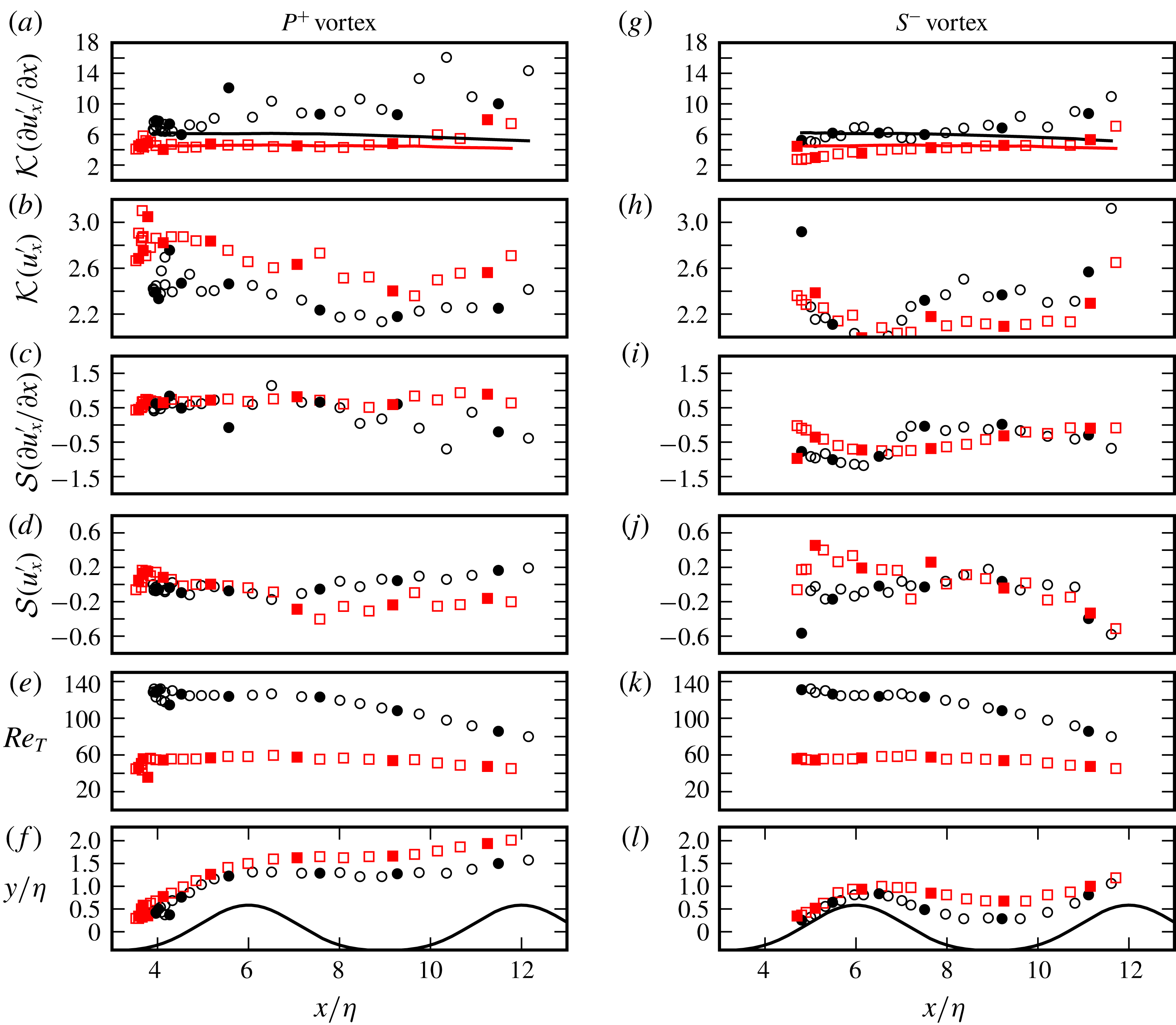
Figure 16. High-order moments (a–d) and (g–j) evaluated on
 $\boldsymbol{x}_{P}(\unicode[STIX]{x1D703})$
(f) for
$\boldsymbol{x}_{P}(\unicode[STIX]{x1D703})$
(f) for
 $4\unicode[STIX]{x03C0}/32\leqslant \unicode[STIX]{x1D703}\leqslant 33\unicode[STIX]{x03C0}/32$
and on
$4\unicode[STIX]{x03C0}/32\leqslant \unicode[STIX]{x1D703}\leqslant 33\unicode[STIX]{x03C0}/32$
and on
 $\boldsymbol{x}_{S}(\unicode[STIX]{x1D703})$
(l) for
$\boldsymbol{x}_{S}(\unicode[STIX]{x1D703})$
(l) for
 $12\unicode[STIX]{x03C0}/32\leqslant \unicode[STIX]{x1D703}\leqslant 33\unicode[STIX]{x03C0}/32$
, cf. table 5 for the details about trajectories
$12\unicode[STIX]{x03C0}/32\leqslant \unicode[STIX]{x1D703}\leqslant 33\unicode[STIX]{x03C0}/32$
, cf. table 5 for the details about trajectories
 $\boldsymbol{x}_{P}(\unicode[STIX]{x1D703})$
and
$\boldsymbol{x}_{P}(\unicode[STIX]{x1D703})$
and
 $\boldsymbol{x}_{S}(\unicode[STIX]{x1D703})$
. The Taylor-microscale Reynolds number (5.5) evaluated on
$\boldsymbol{x}_{S}(\unicode[STIX]{x1D703})$
. The Taylor-microscale Reynolds number (5.5) evaluated on
 $\boldsymbol{x}_{P}(\unicode[STIX]{x1D703})$
(e) and on
$\boldsymbol{x}_{P}(\unicode[STIX]{x1D703})$
(e) and on
 $\boldsymbol{x}_{S}(\unicode[STIX]{x1D703})$
(k). (○): Case C1; (▫): Case C2. Each data point is separated by
$\boldsymbol{x}_{S}(\unicode[STIX]{x1D703})$
(k). (○): Case C1; (▫): Case C2. Each data point is separated by
 $\unicode[STIX]{x03C0}/32$
in time, and filled markers indicate every fourth data point.
$\unicode[STIX]{x03C0}/32$
in time, and filled markers indicate every fourth data point.
 ${\mathcal{K}}$
is the kurtosis,
${\mathcal{K}}$
is the kurtosis,
 ${\mathcal{S}}$
is the skewness.
${\mathcal{S}}$
is the skewness.
Higher-order moments, i.e. the skewness
 ${\mathcal{S}}(a)=\langle a^{3}\rangle /\langle a^{2}\rangle ^{3/2}$
and the kurtosis
${\mathcal{S}}(a)=\langle a^{3}\rangle /\langle a^{2}\rangle ^{3/2}$
and the kurtosis
 ${\mathcal{K}}(a)=\langle a^{4}\rangle /\langle a^{2}\rangle ^{2}$
, of the fluctuating streamwise velocity
${\mathcal{K}}(a)=\langle a^{4}\rangle /\langle a^{2}\rangle ^{2}$
, of the fluctuating streamwise velocity
 $u_{x}^{\prime }$
and of its streamwise derivative
$u_{x}^{\prime }$
and of its streamwise derivative
 $\unicode[STIX]{x2202}u_{x}^{\prime }/\unicode[STIX]{x2202}x$
are shown in figures 16(a–d) and 16(g–j) along the
$\unicode[STIX]{x2202}u_{x}^{\prime }/\unicode[STIX]{x2202}x$
are shown in figures 16(a–d) and 16(g–j) along the
 $\boldsymbol{x}_{P}(\unicode[STIX]{x1D703})$
and
$\boldsymbol{x}_{P}(\unicode[STIX]{x1D703})$
and
 $\boldsymbol{x}_{S}(\unicode[STIX]{x1D703})$
trajectories, respectively. Furthermore, the Taylor-microscale Reynolds number
$\boldsymbol{x}_{S}(\unicode[STIX]{x1D703})$
trajectories, respectively. Furthermore, the Taylor-microscale Reynolds number
 $$\begin{eqnarray}Re_{T}=u^{\prime }\unicode[STIX]{x1D706}_{T}/\unicode[STIX]{x1D708},\end{eqnarray}$$
where
 $u^{\prime }=\sqrt{2k/3}$
and
$u^{\prime }=\sqrt{2k/3}$
and
 $\unicode[STIX]{x1D706}_{T}=\sqrt{10\unicode[STIX]{x1D708}k/\unicode[STIX]{x1D700}}$
, is also evaluated along the trajectories, cf. figures 16(e) and 16(k).
$\unicode[STIX]{x1D706}_{T}=\sqrt{10\unicode[STIX]{x1D708}k/\unicode[STIX]{x1D700}}$
, is also evaluated along the trajectories, cf. figures 16(e) and 16(k).
Figures 16(a,c) and 16(g,i) show that the velocity derivatives deviate from Gaussianity (
 ${\mathcal{S}}=0$
,
${\mathcal{S}}=0$
,
 ${\mathcal{K}}=3$
in a Gaussian distribution) in both vortex cores. The deviation is particularly strong in kurtosis, which is typical for developed turbulent flows due to their internal intermittency, as first observed by Batchelor & Townsend (Reference Batchelor and Townsend1949). Experimental data showed a Reynolds number dependent variation
${\mathcal{K}}=3$
in a Gaussian distribution) in both vortex cores. The deviation is particularly strong in kurtosis, which is typical for developed turbulent flows due to their internal intermittency, as first observed by Batchelor & Townsend (Reference Batchelor and Townsend1949). Experimental data showed a Reynolds number dependent variation
 ${\mathcal{K}}(\unicode[STIX]{x2202}u_{x}^{\prime }/\unicode[STIX]{x2202}x)=Re_{T}^{3/8}$
for this departure (Van Atta & Antonia Reference Van Atta and Antonia1980). These variations are shown with solid lines in figures 16(a) and 16(g). We see that initially
${\mathcal{K}}(\unicode[STIX]{x2202}u_{x}^{\prime }/\unicode[STIX]{x2202}x)=Re_{T}^{3/8}$
for this departure (Van Atta & Antonia Reference Van Atta and Antonia1980). These variations are shown with solid lines in figures 16(a) and 16(g). We see that initially
 ${\mathcal{K}}(\unicode[STIX]{x2202}u_{x}^{\prime }/\unicode[STIX]{x2202}x)$
in both vortex cores is consistent with experimental values, and follows the
${\mathcal{K}}(\unicode[STIX]{x2202}u_{x}^{\prime }/\unicode[STIX]{x2202}x)$
in both vortex cores is consistent with experimental values, and follows the
 $Re_{T}^{3/8}$
-curves. The kurtosis dramatically increases then in C1 despite the decreasing
$Re_{T}^{3/8}$
-curves. The kurtosis dramatically increases then in C1 despite the decreasing
 $Re_{T}$
, cf.
$Re_{T}$
, cf.
 $x/\unicode[STIX]{x1D702}>6$
in figure 16(a,e) and
$x/\unicode[STIX]{x1D702}>6$
in figure 16(a,e) and
 $x/\unicode[STIX]{x1D702}>8$
in figure 16(g,k). High values in the range of
$x/\unicode[STIX]{x1D702}>8$
in figure 16(g,k). High values in the range of
 ${\mathcal{K}}(\unicode[STIX]{x2202}u_{x}^{\prime }/\unicode[STIX]{x2202}x)\approx 15$
are reached, showing a stronger departure from Gaussianity than expected in standard fully developed turbulence. This suggests an additional intermittency mechanism on the spanwise-vortex column. We will see in § 6 that the spanwise vortices disintegrate into large-scale vortex clusters with relatively quiet regions in between, which is indicative of external intermittency. The vortices in C2 do not develop such a strong external intermittency, and the departures from experimental values of kurtosis are relatively modest.
${\mathcal{K}}(\unicode[STIX]{x2202}u_{x}^{\prime }/\unicode[STIX]{x2202}x)\approx 15$
are reached, showing a stronger departure from Gaussianity than expected in standard fully developed turbulence. This suggests an additional intermittency mechanism on the spanwise-vortex column. We will see in § 6 that the spanwise vortices disintegrate into large-scale vortex clusters with relatively quiet regions in between, which is indicative of external intermittency. The vortices in C2 do not develop such a strong external intermittency, and the departures from experimental values of kurtosis are relatively modest.
Figures 16(b) and 16(h) further show that
 ${\mathcal{K}}(u_{x}^{\prime })<3$
for all of the trajectories (except for some initial points of
${\mathcal{K}}(u_{x}^{\prime })<3$
for all of the trajectories (except for some initial points of
 $P^{+}$
in C2). This shows that the probability density functions (PDFs) of the streamwise velocity are more flat than the normal distribution, i.e. high deviations from the mean value are rarer than for a random Gaussian variable. Furthermore, PDFs of the streamwise velocities are in general skewed. In particular,
$P^{+}$
in C2). This shows that the probability density functions (PDFs) of the streamwise velocity are more flat than the normal distribution, i.e. high deviations from the mean value are rarer than for a random Gaussian variable. Furthermore, PDFs of the streamwise velocities are in general skewed. In particular,
 $S^{-}$
-cores show pronounced negative skewness, when
$S^{-}$
-cores show pronounced negative skewness, when
 $S^{-}$
arrives at the neighbouring ripple, cf.
$S^{-}$
arrives at the neighbouring ripple, cf.
 $x/\unicode[STIX]{x1D702}>9$
in figure 16(j).
$x/\unicode[STIX]{x1D702}>9$
in figure 16(j).
5.3 Statistics of the wall shear stress
A significant quantity for sediment-transport processes is the imposed shear stress on the ripple surface. In § 3, we analysed a related quantity, i.e. the spanwise wall vorticity (cf. figure 6). The local phase-averaged tangential shear stress, simply the wall shear stress, on the ripple surface
 $\unicode[STIX]{x1D6FA}_{\unicode[STIX]{x1D702}}$
can be calculated using the wall vorticity as follows
$\unicode[STIX]{x1D6FA}_{\unicode[STIX]{x1D702}}$
can be calculated using the wall vorticity as follows
 $$\begin{eqnarray}\langle \unicode[STIX]{x1D70F}_{t}(\boldsymbol{x},\unicode[STIX]{x1D703})\rangle =-\unicode[STIX]{x1D708}\langle \unicode[STIX]{x1D714}_{z}(\boldsymbol{x},\unicode[STIX]{x1D703})\rangle \quad \text{for }\boldsymbol{x}\in \unicode[STIX]{x1D6FA}_{\unicode[STIX]{x1D702}}.\end{eqnarray}$$
Using the Reynolds decomposition, the instantaneous wall shear stress can be written as
 $\unicode[STIX]{x1D70F}_{t}=\langle \unicode[STIX]{x1D70F}_{t}\rangle +\unicode[STIX]{x1D70F}_{t}^{\prime }$
, where
$\unicode[STIX]{x1D70F}_{t}=\langle \unicode[STIX]{x1D70F}_{t}\rangle +\unicode[STIX]{x1D70F}_{t}^{\prime }$
, where
 $\unicode[STIX]{x1D70F}_{t}^{\prime }$
is the fluctuating part.
$\unicode[STIX]{x1D70F}_{t}^{\prime }$
is the fluctuating part.
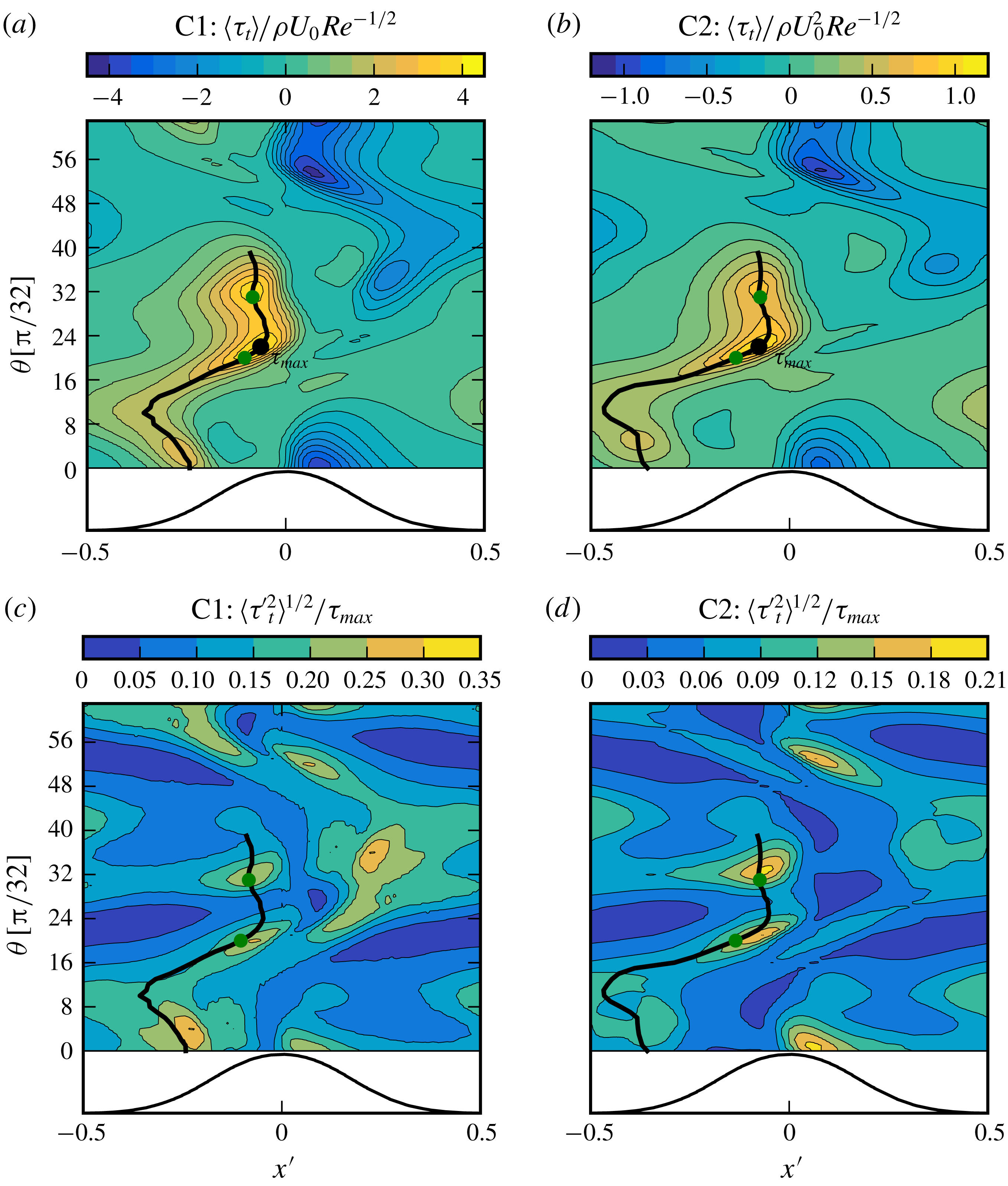
Figure 17. Distribution of the phase-averaged wall shear stress
 $\langle \unicode[STIX]{x1D70F}_{t}\rangle$
(a,b) and its fluctuation intensity
$\langle \unicode[STIX]{x1D70F}_{t}\rangle$
(a,b) and its fluctuation intensity
 $\langle \unicode[STIX]{x1D70F}_{t}^{\prime 2}\rangle ^{1/2}$
(c,d). The location of the global maximum of the wall shear stress, i.e.
$\langle \unicode[STIX]{x1D70F}_{t}^{\prime 2}\rangle ^{1/2}$
(c,d). The location of the global maximum of the wall shear stress, i.e.
 $\unicode[STIX]{x1D70F}_{max}:=\max \{\langle \unicode[STIX]{x1D70F}_{t}(\boldsymbol{x},\unicode[STIX]{x1D703})\rangle \}$
, is indicated by the black markers in (a,b). The intensities are normalized by this value in the respective cases. The thick solid lines go through the phase maxima of the local wall shear stress. The probability density functions of
$\unicode[STIX]{x1D70F}_{max}:=\max \{\langle \unicode[STIX]{x1D70F}_{t}(\boldsymbol{x},\unicode[STIX]{x1D703})\rangle \}$
, is indicated by the black markers in (a,b). The intensities are normalized by this value in the respective cases. The thick solid lines go through the phase maxima of the local wall shear stress. The probability density functions of
 $\unicode[STIX]{x1D70F}_{t}$
at the locations shown with green markers are plotted in figure 19.
$\unicode[STIX]{x1D70F}_{t}$
at the locations shown with green markers are plotted in figure 19.
Figure 17 shows the distribution of the wall shear stress and its fluctuation intensity over the period. The values in figure 17(a,b) are normalized by
 $\unicode[STIX]{x1D70F}_{max}^{f}=\unicode[STIX]{x1D70C}U_{0}^{2}Re^{-1/2}$
, which is the maximum value for the wall shear stress in a laminar sinusoidal oscillatory flow over a flat smooth wall (Batchelor Reference Batchelor2000). The laminar scaling is selected, as Reynolds numbers in this work are below the transition Reynolds number (
$\unicode[STIX]{x1D70F}_{max}^{f}=\unicode[STIX]{x1D70C}U_{0}^{2}Re^{-1/2}$
, which is the maximum value for the wall shear stress in a laminar sinusoidal oscillatory flow over a flat smooth wall (Batchelor Reference Batchelor2000). The laminar scaling is selected, as Reynolds numbers in this work are below the transition Reynolds number (
 $Re\approx 40\,000$
, cf. Jensen, Sumer & Fredsoe (Reference Jensen, Sumer and Fredsoe1989)) of the smooth bottom oscillatory boundary layer. The regions with intense shear are of most practical interest, as they imply regions prone to active sediment motion. In order to elaborate the statistics in these regions, we define a high-shear trajectory
$Re\approx 40\,000$
, cf. Jensen, Sumer & Fredsoe (Reference Jensen, Sumer and Fredsoe1989)) of the smooth bottom oscillatory boundary layer. The regions with intense shear are of most practical interest, as they imply regions prone to active sediment motion. In order to elaborate the statistics in these regions, we define a high-shear trajectory
 $\boldsymbol{x}_{\unicode[STIX]{x1D70F}}(\unicode[STIX]{x1D703})$
, which goes through the phase maxima of the wall shear stress at the lee of the ripple. The thick solid lines in figure 17 show the evolution of the trajectory over the ripple for
$\boldsymbol{x}_{\unicode[STIX]{x1D70F}}(\unicode[STIX]{x1D703})$
, which goes through the phase maxima of the wall shear stress at the lee of the ripple. The thick solid lines in figure 17 show the evolution of the trajectory over the ripple for
 $0\leqslant \unicode[STIX]{x1D703}\leqslant 40\unicode[STIX]{x03C0}/32$
. The maximum shear on this trajectory occurs at
$0\leqslant \unicode[STIX]{x1D703}\leqslant 40\unicode[STIX]{x03C0}/32$
. The maximum shear on this trajectory occurs at
 $\boldsymbol{x}_{\unicode[STIX]{x1D70F}}(22\unicode[STIX]{x03C0}/32)$
for both cases. This is the global maximum of the wall shear stress, which will be denoted as
$\boldsymbol{x}_{\unicode[STIX]{x1D70F}}(22\unicode[STIX]{x03C0}/32)$
for both cases. This is the global maximum of the wall shear stress, which will be denoted as
 $\unicode[STIX]{x1D70F}_{max}$
, i.e.
$\unicode[STIX]{x1D70F}_{max}$
, i.e.
 $\unicode[STIX]{x1D70F}_{max}:=\max \{\langle \unicode[STIX]{x1D70F}_{t}(\boldsymbol{x},\unicode[STIX]{x1D703})\rangle \}$
for
$\unicode[STIX]{x1D70F}_{max}:=\max \{\langle \unicode[STIX]{x1D70F}_{t}(\boldsymbol{x},\unicode[STIX]{x1D703})\rangle \}$
for
 $\boldsymbol{x}\in \unicode[STIX]{x1D6FA}_{\unicode[STIX]{x1D702}}$
. The intensities in figure 17(c,d) are normalized by these respective values of
$\boldsymbol{x}\in \unicode[STIX]{x1D6FA}_{\unicode[STIX]{x1D702}}$
. The intensities in figure 17(c,d) are normalized by these respective values of
 $\unicode[STIX]{x1D70F}_{max}$
. Black markers in figure 17(a,b) indicate
$\unicode[STIX]{x1D70F}_{max}$
. Black markers in figure 17(a,b) indicate
 $\unicode[STIX]{x1D70F}_{max}$
for both cases, where
$\unicode[STIX]{x1D70F}_{max}$
for both cases, where
 $\unicode[STIX]{x1D70F}_{max}=4.18\unicode[STIX]{x1D70F}_{max}^{f}$
in Case C1 and
$\unicode[STIX]{x1D70F}_{max}=4.18\unicode[STIX]{x1D70F}_{max}^{f}$
in Case C1 and
 $\unicode[STIX]{x1D70F}_{max}=1.08\unicode[STIX]{x1D70F}_{max}^{f}$
in Case C2. We see an increase in the wall-shear-stress peak with increasing
$\unicode[STIX]{x1D70F}_{max}=1.08\unicode[STIX]{x1D70F}_{max}^{f}$
in Case C2. We see an increase in the wall-shear-stress peak with increasing
 $Re$
in contrast to laminar oscillatory boundary layers over a smooth flat wall, where wall shear stress decays with
$Re$
in contrast to laminar oscillatory boundary layers over a smooth flat wall, where wall shear stress decays with
 $Re^{-1/2}$
.
$Re^{-1/2}$
.
At the start of the period in
 $0\leqslant \unicode[STIX]{x1D703}\leqslant 26\unicode[STIX]{x03C0}/32$
,
$0\leqslant \unicode[STIX]{x1D703}\leqslant 26\unicode[STIX]{x03C0}/32$
,
 $\langle \unicode[STIX]{x1D70F}_{t}(\boldsymbol{x}_{\unicode[STIX]{x1D70F}}(\unicode[STIX]{x1D703}),\unicode[STIX]{x1D703})\rangle$
corresponds to the footprint of the
$\langle \unicode[STIX]{x1D70F}_{t}(\boldsymbol{x}_{\unicode[STIX]{x1D70F}}(\unicode[STIX]{x1D703}),\unicode[STIX]{x1D703})\rangle$
corresponds to the footprint of the
 $P^{+}$
-vortex that is forming and will eventually eject itself in the positive streamwise direction. The relation of these intense shear locations to the motion of the vortex was discussed in § 3;
$P^{+}$
-vortex that is forming and will eventually eject itself in the positive streamwise direction. The relation of these intense shear locations to the motion of the vortex was discussed in § 3;
 $\langle \unicode[STIX]{x1D70F}_{t}\rangle$
reaches its highest values in the range
$\langle \unicode[STIX]{x1D70F}_{t}\rangle$
reaches its highest values in the range
 $16\unicode[STIX]{x03C0}/32\leqslant \unicode[STIX]{x1D703}\leqslant 36\unicode[STIX]{x03C0}/32$
near the ripple crest, cf. figure 17(a,b). Two peaks are observed in this range. The first one is
$16\unicode[STIX]{x03C0}/32\leqslant \unicode[STIX]{x1D703}\leqslant 36\unicode[STIX]{x03C0}/32$
near the ripple crest, cf. figure 17(a,b). Two peaks are observed in this range. The first one is
 $\unicode[STIX]{x1D70F}_{max}$
at
$\unicode[STIX]{x1D70F}_{max}$
at
 $\unicode[STIX]{x1D703}=22\unicode[STIX]{x03C0}/32$
and occurs during the ejection of the vortex pair from the crest. The second peak occurs at
$\unicode[STIX]{x1D703}=22\unicode[STIX]{x03C0}/32$
and occurs during the ejection of the vortex pair from the crest. The second peak occurs at
 $\unicode[STIX]{x1D703}\approx \unicode[STIX]{x03C0}$
, when the free-stream velocity peaks. It is observed that high fluctuation regimes occur near these peaks, cf. figure 17(c,d). The intensities in figure 17(c,d) are normalized by these respective values of
$\unicode[STIX]{x1D703}\approx \unicode[STIX]{x03C0}$
, when the free-stream velocity peaks. It is observed that high fluctuation regimes occur near these peaks, cf. figure 17(c,d). The intensities in figure 17(c,d) are normalized by these respective values of
 $\unicode[STIX]{x1D70F}_{max}$
.
$\unicode[STIX]{x1D70F}_{max}$
.
Figure 18 shows the statistical moments of
 $\unicode[STIX]{x1D70F}_{t}$
on high-shear trajectories
$\unicode[STIX]{x1D70F}_{t}$
on high-shear trajectories
 $\boldsymbol{x}_{\unicode[STIX]{x1D70F}}(\unicode[STIX]{x1D703})$
. Two regimes with high
$\boldsymbol{x}_{\unicode[STIX]{x1D70F}}(\unicode[STIX]{x1D703})$
. Two regimes with high
 $\langle \unicode[STIX]{x1D70F}_{t}\rangle$
and
$\langle \unicode[STIX]{x1D70F}_{t}\rangle$
and
 $\langle \unicode[STIX]{x1D70F}_{t}^{\prime 2}\rangle$
appear as two peaks after
$\langle \unicode[STIX]{x1D70F}_{t}^{\prime 2}\rangle$
appear as two peaks after
 $\unicode[STIX]{x1D703}>16\unicode[STIX]{x03C0}/32$
, cf. figure 18(a,b). The flatness factors (figure 18
c) and the skewness factors (figure 18
d) show that these two intense shear regimes have very different fluctuation characteristics. There is a dramatic rise in the skewness and flatness in the second high-stress regime, which takes place at approximately
$\unicode[STIX]{x1D703}>16\unicode[STIX]{x03C0}/32$
, cf. figure 18(a,b). The flatness factors (figure 18
c) and the skewness factors (figure 18
d) show that these two intense shear regimes have very different fluctuation characteristics. There is a dramatic rise in the skewness and flatness in the second high-stress regime, which takes place at approximately
 $27\unicode[STIX]{x03C0}/32<\unicode[STIX]{x1D703}<34\unicode[STIX]{x03C0}/32$
. This rise, occurring slightly ahead of the rise in the first- and second-order moments, leads to strong departures from a normal distribution in the PDFs,
$27\unicode[STIX]{x03C0}/32<\unicode[STIX]{x1D703}<34\unicode[STIX]{x03C0}/32$
. This rise, occurring slightly ahead of the rise in the first- and second-order moments, leads to strong departures from a normal distribution in the PDFs,
 $f(\unicode[STIX]{x1D70F}_{t})$
. This is shown in figure 19 using PDFs at two different phases: an instance in the vortex-ejection regime at
$f(\unicode[STIX]{x1D70F}_{t})$
. This is shown in figure 19 using PDFs at two different phases: an instance in the vortex-ejection regime at
 $\boldsymbol{x}_{\unicode[STIX]{x1D70F}}(20\unicode[STIX]{x03C0}/32)$
and another instance in the high free-stream velocity regime at
$\boldsymbol{x}_{\unicode[STIX]{x1D70F}}(20\unicode[STIX]{x03C0}/32)$
and another instance in the high free-stream velocity regime at
 $\boldsymbol{x}_{\unicode[STIX]{x1D70F}}(31\unicode[STIX]{x03C0}/32)$
. These selected points on
$\boldsymbol{x}_{\unicode[STIX]{x1D70F}}(31\unicode[STIX]{x03C0}/32)$
. These selected points on
 $\boldsymbol{x}_{\unicode[STIX]{x1D70F}}$
are indicated by the green markers in figure 17. We see that the PDFs at
$\boldsymbol{x}_{\unicode[STIX]{x1D70F}}$
are indicated by the green markers in figure 17. We see that the PDFs at
 $\unicode[STIX]{x1D703}=31\unicode[STIX]{x03C0}/32$
show high positive skewness with long tails, so the mean values do not have the highest probability density.
$\unicode[STIX]{x1D703}=31\unicode[STIX]{x03C0}/32$
show high positive skewness with long tails, so the mean values do not have the highest probability density.
The strongly non-Gaussian range in
 $27\unicode[STIX]{x03C0}/32<\unicode[STIX]{x1D703}<34\unicode[STIX]{x03C0}/32$
is related to the passage of the
$27\unicode[STIX]{x03C0}/32<\unicode[STIX]{x1D703}<34\unicode[STIX]{x03C0}/32$
is related to the passage of the
 $P^{+}$
–
$P^{+}$
–
 $S^{-}$
vortices from the previous half-cycle over the ripple crest. Therefore, the positively skewed fluctuations with long tails appear to be imposed by these vortices.
$S^{-}$
vortices from the previous half-cycle over the ripple crest. Therefore, the positively skewed fluctuations with long tails appear to be imposed by these vortices.

Figure 18. Central moments of the wall shear stress evaluated on a high-shear trajectory
 $\boldsymbol{x}_{\unicode[STIX]{x1D70F}}(\unicode[STIX]{x1D703})$
, cf. thick lines in figure 17. (a) Mean value scaled with
$\boldsymbol{x}_{\unicode[STIX]{x1D70F}}(\unicode[STIX]{x1D703})$
, cf. thick lines in figure 17. (a) Mean value scaled with
 $\unicode[STIX]{x1D70F}_{max}:=\max \{\langle \unicode[STIX]{x1D70F}_{t}(\boldsymbol{x},\unicode[STIX]{x1D703})\rangle \}$
; (b) fluctuation intensity scaled with
$\unicode[STIX]{x1D70F}_{max}:=\max \{\langle \unicode[STIX]{x1D70F}_{t}(\boldsymbol{x},\unicode[STIX]{x1D703})\rangle \}$
; (b) fluctuation intensity scaled with
 $\unicode[STIX]{x1D70F}_{max}$
; (c) the skewness factor
$\unicode[STIX]{x1D70F}_{max}$
; (c) the skewness factor
 ${\mathcal{S}}(\unicode[STIX]{x1D70F}_{t}^{\prime })=\langle \unicode[STIX]{x1D70F}_{t}^{\prime 3}\rangle /\langle \unicode[STIX]{x1D70F}_{t}^{\prime 2}\rangle ^{3/2}$
; (d) the flatness factor
${\mathcal{S}}(\unicode[STIX]{x1D70F}_{t}^{\prime })=\langle \unicode[STIX]{x1D70F}_{t}^{\prime 3}\rangle /\langle \unicode[STIX]{x1D70F}_{t}^{\prime 2}\rangle ^{3/2}$
; (d) the flatness factor
 ${\mathcal{F}}(\unicode[STIX]{x1D70F}_{t}^{\prime })=\langle \unicode[STIX]{x1D70F}_{t}^{\prime 4}\rangle /\langle \unicode[STIX]{x1D70F}_{t}^{\prime 2}\rangle ^{2}$
. (○) Case C1; (▫) Case C2. The filled markers indicate the selected phases for the presentation of PDFs in figure 19.
${\mathcal{F}}(\unicode[STIX]{x1D70F}_{t}^{\prime })=\langle \unicode[STIX]{x1D70F}_{t}^{\prime 4}\rangle /\langle \unicode[STIX]{x1D70F}_{t}^{\prime 2}\rangle ^{2}$
. (○) Case C1; (▫) Case C2. The filled markers indicate the selected phases for the presentation of PDFs in figure 19.

Figure 19. Probability density functions (PDFs) of the local wall shear stress,
 $f(\unicode[STIX]{x1D70F}_{t})$
, evaluated at
$f(\unicode[STIX]{x1D70F}_{t})$
, evaluated at
 $\boldsymbol{x}_{\unicode[STIX]{x1D70F}}(20\unicode[STIX]{x03C0}/32)$
and
$\boldsymbol{x}_{\unicode[STIX]{x1D70F}}(20\unicode[STIX]{x03C0}/32)$
and
 $\boldsymbol{x}_{\unicode[STIX]{x1D70F}}(31\unicode[STIX]{x03C0}/32)$
. The selected points are indicated with green markers in figure 17. Markers show the PDFs of mean values, i.e.
$\boldsymbol{x}_{\unicode[STIX]{x1D70F}}(31\unicode[STIX]{x03C0}/32)$
. The selected points are indicated with green markers in figure 17. Markers show the PDFs of mean values, i.e.
 $f(\langle \unicode[STIX]{x1D70F}_{t}(\boldsymbol{x}_{\unicode[STIX]{x1D70F}}(\unicode[STIX]{x1D703}),\unicode[STIX]{x1D703})\rangle )$
. Sample spaces are normalized with the global maximum of the wall shear stress, i.e.
$f(\langle \unicode[STIX]{x1D70F}_{t}(\boldsymbol{x}_{\unicode[STIX]{x1D70F}}(\unicode[STIX]{x1D703}),\unicode[STIX]{x1D703})\rangle )$
. Sample spaces are normalized with the global maximum of the wall shear stress, i.e.
 $\unicode[STIX]{x1D70F}_{max}:=\max \{\langle \unicode[STIX]{x1D70F}_{t}(\boldsymbol{x},\unicode[STIX]{x1D703})\rangle \}$
, cf. black markers in figure 17(a,b).
$\unicode[STIX]{x1D70F}_{max}:=\max \{\langle \unicode[STIX]{x1D70F}_{t}(\boldsymbol{x},\unicode[STIX]{x1D703})\rangle \}$
, cf. black markers in figure 17(a,b).
6 Three-dimensional structures
The main structural elements of the flow are the coherent spanwise vortices whose two-dimensional phase-averaged statistics were studied in the previous sections. The observations in § 5.2 suggested that these vortices lose their spanwise coherence and would develop external intermittency. Furthermore, the resulting intermittent features appear to have an influence on the non-Gaussian wall-shear-stress fields when they arrive at the neighbouring ripple. In this section, we provide visual evidence for these results, and also conduct further statistical analyses using the transverse spectra of the fluctuating fields along the vortex trajectories. To this end, we focus on the energetic vortex modes responsible for the breakdown of spanwise coherence. We have further observed in § 5.2 (cf. figure 14
g,h) that anisotropies in the fluctuating fields increase drastically in the near-wall region when the
 $P$
–
$P$
–
 $S$
dipole moves over the crest. This suggested that coherent structures with strong alignment to one direction dominate the near-wall layer in this phase. We will also study these near-wall turbulent structures and their footprints on wall-shear-stress fluctuations.
$S$
dipole moves over the crest. This suggested that coherent structures with strong alignment to one direction dominate the near-wall layer in this phase. We will also study these near-wall turbulent structures and their footprints on wall-shear-stress fluctuations.
6.1 Three-dimensional visualization of instantaneous flow fields
We start our analysis with three-dimensional visualizations of the instantaneous flow. Only the fluctuating fields are considered, as we have discussed the motion of Reynolds-averaged fields in detail in § 3. We focus on the ejection phase (
 $\unicode[STIX]{x1D703}\geqslant \unicode[STIX]{x03C0}/2$
). The spanwise vortices in the vortex-formation phase (
$\unicode[STIX]{x1D703}\geqslant \unicode[STIX]{x03C0}/2$
). The spanwise vortices in the vortex-formation phase (
 $\unicode[STIX]{x1D703}<\unicode[STIX]{x03C0}/2$
) remain relatively immobile at the lee side, and their footprints on the ripple surface are mild until their ejection over the ripple (cf. the discussion in § 5.3). Therefore, their structural features in the vortex-formation phase are of less importance, and are not presented here for brevity. A more complete picture including the vortex-formation phase will be given in the spectral analysis of § 6.2.
$\unicode[STIX]{x1D703}<\unicode[STIX]{x03C0}/2$
) remain relatively immobile at the lee side, and their footprints on the ripple surface are mild until their ejection over the ripple (cf. the discussion in § 5.3). Therefore, their structural features in the vortex-formation phase are of less importance, and are not presented here for brevity. A more complete picture including the vortex-formation phase will be given in the spectral analysis of § 6.2.
In order to extract the flow structures, we employ the second invariant of the fluctuating velocity gradient tensor, i.e.
 $$\begin{eqnarray}Q={\textstyle \frac{1}{2}}(\unicode[STIX]{x1D6FA}_{ij}^{\prime }\unicode[STIX]{x1D6FA}_{ij}^{\prime }-\unicode[STIX]{x1D634}_{ij}^{\prime }\unicode[STIX]{x1D634}_{ij}^{\prime }),\end{eqnarray}$$
where
 $\unicode[STIX]{x1D6FA}_{ij}^{\prime }=1/2(\unicode[STIX]{x2202}u_{i}^{\prime }/\unicode[STIX]{x2202}x_{j}-\unicode[STIX]{x2202}u_{j}^{\prime }/\unicode[STIX]{x2202}x_{i})$
is the fluctuating rate of spin tensor. The
$\unicode[STIX]{x1D6FA}_{ij}^{\prime }=1/2(\unicode[STIX]{x2202}u_{i}^{\prime }/\unicode[STIX]{x2202}x_{j}-\unicode[STIX]{x2202}u_{j}^{\prime }/\unicode[STIX]{x2202}x_{i})$
is the fluctuating rate of spin tensor. The
 $Q$
-invariant extracted from fluctuating fields is usually employed to analyse inhomogeneous turbulent flows, e.g. Gomes-Fernandes, Ganapathisubramani & Vassilicos (Reference Gomes-Fernandes, Ganapathisubramani and Vassilicos2014) and Buxton, Breda & Chen (Reference Buxton, Breda and Chen2017). Positive values of
$Q$
-invariant extracted from fluctuating fields is usually employed to analyse inhomogeneous turbulent flows, e.g. Gomes-Fernandes, Ganapathisubramani & Vassilicos (Reference Gomes-Fernandes, Ganapathisubramani and Vassilicos2014) and Buxton, Breda & Chen (Reference Buxton, Breda and Chen2017). Positive values of
 $Q$
occur in the regions where the fluctuating vorticity dominates over the fluctuating strain. These regions are intense in enstrophy. Similarly, negative values of
$Q$
occur in the regions where the fluctuating vorticity dominates over the fluctuating strain. These regions are intense in enstrophy. Similarly, negative values of
 $Q$
occur in strain-dominated regions, which are strongly dissipative. Both strain and vorticity are essential in the turbulent dynamics, as the term
$Q$
occur in strain-dominated regions, which are strongly dissipative. Both strain and vorticity are essential in the turbulent dynamics, as the term
 $\unicode[STIX]{x1D714}_{i}^{\prime }\unicode[STIX]{x1D714}_{j}^{\prime }\unicode[STIX]{x1D634}_{ij}^{\prime }$
is the main driver of the enstrophy production and the turbulent cascade (Tennekes & Lumley Reference Tennekes and Lumley1972). We have observed in our simulations that large values of positive and negative
$\unicode[STIX]{x1D714}_{i}^{\prime }\unicode[STIX]{x1D714}_{j}^{\prime }\unicode[STIX]{x1D634}_{ij}^{\prime }$
is the main driver of the enstrophy production and the turbulent cascade (Tennekes & Lumley Reference Tennekes and Lumley1972). We have observed in our simulations that large values of positive and negative
 $Q$
concentrate in the same regions. Therefore, we use merely the positive isosurfaces of
$Q$
concentrate in the same regions. Therefore, we use merely the positive isosurfaces of
 $Q$
to visualize dynamically active regions. The regions of intense strain usually neighbour the visualized regions, and are not discussed below for brevity.
$Q$
to visualize dynamically active regions. The regions of intense strain usually neighbour the visualized regions, and are not discussed below for brevity.

Figure 20. Isosurfaces of
 $Q$
parameter (cf. (6.1)) at three different instances
$Q$
parameter (cf. (6.1)) at three different instances
 $\unicode[STIX]{x1D703}=20\unicode[STIX]{x03C0}/32,26\unicode[STIX]{x03C0}/32,31\unicode[STIX]{x03C0}/32$
. Surfaces are coloured based on streamwise-velocity fluctuations
$\unicode[STIX]{x1D703}=20\unicode[STIX]{x03C0}/32,26\unicode[STIX]{x03C0}/32,31\unicode[STIX]{x03C0}/32$
. Surfaces are coloured based on streamwise-velocity fluctuations
 $u_{x}^{\prime }$
. The flows are convected from left to right. (a,c,e) Case C1,
$u_{x}^{\prime }$
. The flows are convected from left to right. (a,c,e) Case C1,
 $Q=40(U_{0}/\unicode[STIX]{x1D702})^{2}$
; (b,d,f) Case C2,
$Q=40(U_{0}/\unicode[STIX]{x1D702})^{2}$
; (b,d,f) Case C2,
 $Q=3.2(U_{0}/\unicode[STIX]{x1D702})^{2}$
. Black circles in (a,c,e) show the evolution of a high-momentum structure. Red ellipses in (a–d) indicate an instance of streamwise-oriented vortical structures.
$Q=3.2(U_{0}/\unicode[STIX]{x1D702})^{2}$
. Black circles in (a,c,e) show the evolution of a high-momentum structure. Red ellipses in (a–d) indicate an instance of streamwise-oriented vortical structures.
Figure 20 demonstrates intensive enstrophy regions in a selected subdomain for three different phases at
 $\unicode[STIX]{x1D703}=20\unicode[STIX]{x03C0}/32,26\unicode[STIX]{x03C0}/32,31\unicode[STIX]{x03C0}/32$
. The isosurfaces are coloured with the fluctuating streamwise velocity
$\unicode[STIX]{x1D703}=20\unicode[STIX]{x03C0}/32,26\unicode[STIX]{x03C0}/32,31\unicode[STIX]{x03C0}/32$
. The isosurfaces are coloured with the fluctuating streamwise velocity
 $u_{x}^{\prime }$
. We see that during their ejection from the crest at
$u_{x}^{\prime }$
. We see that during their ejection from the crest at
 $\unicode[STIX]{x1D703}=20\unicode[STIX]{x03C0}/32$
, the
$\unicode[STIX]{x1D703}=20\unicode[STIX]{x03C0}/32$
, the
 $P^{+}$
and
$P^{+}$
and
 $S^{-}$
vortices are in the form of turbulent vortex clouds that span the entire lateral dimension of the selected subdomain (also of the entire computational domain, not shown here), cf. figure 20(a,b). In C1, there are large regions on the vortex cloud that are predominantly in red, i.e. have a higher velocity than its surrounding. These regions indicate the presence of an unstable vortex mode on the vortex column, which gives rise to large-scale high-momentum structures with spanwise dimensions of approximately
$S^{-}$
vortices are in the form of turbulent vortex clouds that span the entire lateral dimension of the selected subdomain (also of the entire computational domain, not shown here), cf. figure 20(a,b). In C1, there are large regions on the vortex cloud that are predominantly in red, i.e. have a higher velocity than its surrounding. These regions indicate the presence of an unstable vortex mode on the vortex column, which gives rise to large-scale high-momentum structures with spanwise dimensions of approximately
 $3\unicode[STIX]{x1D702}-4\unicode[STIX]{x1D702}$
. One instance of these high-momentum structures is marked with a black circle in figure 20(a). These structures cannot be easily identified in C2 with the selected visualization method. However, we will see in spectral analysis in § 6.2 that a dominant vortex mode also exists in C2.
$3\unicode[STIX]{x1D702}-4\unicode[STIX]{x1D702}$
. One instance of these high-momentum structures is marked with a black circle in figure 20(a). These structures cannot be easily identified in C2 with the selected visualization method. However, we will see in spectral analysis in § 6.2 that a dominant vortex mode also exists in C2.
In addition to large-scale momentum structures on the vortex column, there are also organized features near the wall in the form of streamwise-oriented elongated vortex pairs. Two examples are indicated with red ellipses in figure 20(a,b). In C2, these vortices are arranged in a somewhat regular fashion along the entire spanwise extent (figure 20 b). In contrast, in C1 they concentrate preferably in the trail of high-momentum structures (figure 20 a). These streamwise-aligned longitudinal structures are responsible for the highly anisotropic near-wall layers observed in the statistical analysis of § 5.2 (cf. figure 14 g,h).
When the coherent spanwise vortices detach themselves from the ripple crest, the streamwise structures are still observable in their trail around the crest, cf. red ellipses at
 $\unicode[STIX]{x1D703}=26\unicode[STIX]{x03C0}/32$
in figure 20(c,d). We further see in this phase that the high-momentum structure (black circle) in C1 keeps its coherence, whereas low-momentum regions (blue parts) around it become slowly depleted in intense vortical structures.
$\unicode[STIX]{x1D703}=26\unicode[STIX]{x03C0}/32$
in figure 20(c,d). We further see in this phase that the high-momentum structure (black circle) in C1 keeps its coherence, whereas low-momentum regions (blue parts) around it become slowly depleted in intense vortical structures.
Figure 20(e,f) show the phase
 $\unicode[STIX]{x1D703}=31\unicode[STIX]{x03C0}/32$
when the vortex clouds arrive at the crest of the neighbouring ripple. These structures show quite different characteristics in C1 and C2. We see in figure 20(e) that vortical structures in C1 survive only in the regions with high fluctuating velocity (marked with solid circle) and are mostly depleted in low velocity regions (marked with dotted circle). As the regions between high-momentum structures are relatively quiet in terms of intense vortical structures and strain structures (not shown here), the flow can be considered intermittent in the spanwise direction. Namely, small-scale turbulence preferentially concentrates in regions with positive fluctuating velocity. We denote the final isolated form of the high-momentum structure as a turbulent vortex cluster. Turbulent vortex clusters seem to have the tendency to be arranged in staggered patterns, such that there is a spanwise shift between the neighbouring vortex clusters in the streamwise direction. Such an arrangement is reminiscent of a brick pattern. The clustering of highly vortical elements in high-momentum structures is not observed in C2 (figure 20
f). These observations provide a visual perspective for the relatively high kurtosis in the velocity derivative
$\unicode[STIX]{x1D703}=31\unicode[STIX]{x03C0}/32$
when the vortex clouds arrive at the crest of the neighbouring ripple. These structures show quite different characteristics in C1 and C2. We see in figure 20(e) that vortical structures in C1 survive only in the regions with high fluctuating velocity (marked with solid circle) and are mostly depleted in low velocity regions (marked with dotted circle). As the regions between high-momentum structures are relatively quiet in terms of intense vortical structures and strain structures (not shown here), the flow can be considered intermittent in the spanwise direction. Namely, small-scale turbulence preferentially concentrates in regions with positive fluctuating velocity. We denote the final isolated form of the high-momentum structure as a turbulent vortex cluster. Turbulent vortex clusters seem to have the tendency to be arranged in staggered patterns, such that there is a spanwise shift between the neighbouring vortex clusters in the streamwise direction. Such an arrangement is reminiscent of a brick pattern. The clustering of highly vortical elements in high-momentum structures is not observed in C2 (figure 20
f). These observations provide a visual perspective for the relatively high kurtosis in the velocity derivative
 $\unicode[STIX]{x2202}u_{x}^{\prime }/\unicode[STIX]{x2202}x$
(a small-scale quantity like
$\unicode[STIX]{x2202}u_{x}^{\prime }/\unicode[STIX]{x2202}x$
(a small-scale quantity like
 $Q$
) compared with the standard values in fully developed turbulence at vortex cores of C1 (cf. figures 16.Ia and 16.IIa). As the external intermittency is not strong in C2, the small-scale kurtosis in C2 remains close to fully developed turbulence values, cf. the discussion in § 5.2.
$Q$
) compared with the standard values in fully developed turbulence at vortex cores of C1 (cf. figures 16.Ia and 16.IIa). As the external intermittency is not strong in C2, the small-scale kurtosis in C2 remains close to fully developed turbulence values, cf. the discussion in § 5.2.

Figure 21. Footprints of turbulent vortex clusters on the wall shear stress for Case C1. (a,c) Wall-shear-stress fluctuations
 $\unicode[STIX]{x1D70F}_{t}^{\prime }/\unicode[STIX]{x1D70F}_{max}$
; (b,d) top view of
$\unicode[STIX]{x1D70F}_{t}^{\prime }/\unicode[STIX]{x1D70F}_{max}$
; (b,d) top view of
 $Q$
-isosurfaces coloured with streamwise-velocity fluctuations
$Q$
-isosurfaces coloured with streamwise-velocity fluctuations
 $u_{x}^{\prime }$
. Circles in (a,b) and (c,d) mark a large-scale structure and its footprint on the wall shear stress. Dashed lines show the ripple crests, and dotted lines in (a,c) show the location of maximum phase-averaged wall shear stress (
$u_{x}^{\prime }$
. Circles in (a,b) and (c,d) mark a large-scale structure and its footprint on the wall shear stress. Dashed lines show the ripple crests, and dotted lines in (a,c) show the location of maximum phase-averaged wall shear stress (
 $\langle \unicode[STIX]{x1D70F}_{t}\rangle$
).
$\langle \unicode[STIX]{x1D70F}_{t}\rangle$
).
Large-scale momentum structures have strong footprints on the wall. This is shown in figure 21 for Case C1 at phases
 $\unicode[STIX]{x1D703}=20\unicode[STIX]{x03C0}/32,31\unicode[STIX]{x03C0}/32$
. These phases are in the regimes where the peak values of wall shear stress and its fluctuation occur (cf. figure 17
a,c). The dotted lines in figure 21(a,c) indicate the locations on the ripple where the phase-averaged wall shear stress peaks at the respective phase, i.e.
$\unicode[STIX]{x1D703}=20\unicode[STIX]{x03C0}/32,31\unicode[STIX]{x03C0}/32$
. These phases are in the regimes where the peak values of wall shear stress and its fluctuation occur (cf. figure 17
a,c). The dotted lines in figure 21(a,c) indicate the locations on the ripple where the phase-averaged wall shear stress peaks at the respective phase, i.e.
 $\boldsymbol{x}_{\unicode[STIX]{x1D70F}}(20\unicode[STIX]{x03C0}/32)$
and
$\boldsymbol{x}_{\unicode[STIX]{x1D70F}}(20\unicode[STIX]{x03C0}/32)$
and
 $\boldsymbol{x}_{\unicode[STIX]{x1D70F}}(31\unicode[STIX]{x03C0}/32)$
(cf. the green markers in figure 17
a). It is observed at
$\boldsymbol{x}_{\unicode[STIX]{x1D70F}}(31\unicode[STIX]{x03C0}/32)$
(cf. the green markers in figure 17
a). It is observed at
 $\unicode[STIX]{x1D703}=20\unicode[STIX]{x03C0}/32$
that wall-shear-stress fluctuations closely follow the large-scale patterns in the spanwise vortex. One instance of this relation is marked with circles in figure 21(a,b). A high shear-stress region with circa
$\unicode[STIX]{x1D703}=20\unicode[STIX]{x03C0}/32$
that wall-shear-stress fluctuations closely follow the large-scale patterns in the spanwise vortex. One instance of this relation is marked with circles in figure 21(a,b). A high shear-stress region with circa
 $3\unicode[STIX]{x1D702}-4\unicode[STIX]{x1D702}$
width is observed in figure 21(a), which is at the footprint of a high-momentum structure indicated in figure 21(b). Furthermore, the selected high-stress region also features narrow stripy patterns elongated in the streamwise direction, which are produced by near-wall streamwise vortices and accompanying low-speed streaks.
$3\unicode[STIX]{x1D702}-4\unicode[STIX]{x1D702}$
width is observed in figure 21(a), which is at the footprint of a high-momentum structure indicated in figure 21(b). Furthermore, the selected high-stress region also features narrow stripy patterns elongated in the streamwise direction, which are produced by near-wall streamwise vortices and accompanying low-speed streaks.
At
 $\unicode[STIX]{x1D703}=31\unicode[STIX]{x03C0}/32$
, turbulent vortex clusters sweep the neighbouring ripple and induce large-scale fluctuations in wall shear stress in this process. One instance of this event is indicated with circles in figure 21(c,d). The induced fluctuations due to sweeping are significantly more intense than the ones observed during the ejection of the vortex cloud (note the different range employed in colour bars of figure 21
a,c). Outside the contact regions with the vortex cluster, the shear-stress fluctuations appear negative and relatively weak.
$\unicode[STIX]{x1D703}=31\unicode[STIX]{x03C0}/32$
, turbulent vortex clusters sweep the neighbouring ripple and induce large-scale fluctuations in wall shear stress in this process. One instance of this event is indicated with circles in figure 21(c,d). The induced fluctuations due to sweeping are significantly more intense than the ones observed during the ejection of the vortex cloud (note the different range employed in colour bars of figure 21
a,c). Outside the contact regions with the vortex cluster, the shear-stress fluctuations appear negative and relatively weak.

Figure 22. Instantaneous signals on the spanwise line at three selected locations at phase
 $31\unicode[STIX]{x03C0}/32$
. (a) Streamwise velocity at the primary vortex core,
$31\unicode[STIX]{x03C0}/32$
. (a) Streamwise velocity at the primary vortex core,
 $u_{x}^{\prime }(\boldsymbol{x}_{P}(31\unicode[STIX]{x03C0}/32),z,31\unicode[STIX]{x03C0}/32)$
; (b) streamwise velocity at the secondary vortex core,
$u_{x}^{\prime }(\boldsymbol{x}_{P}(31\unicode[STIX]{x03C0}/32),z,31\unicode[STIX]{x03C0}/32)$
; (b) streamwise velocity at the secondary vortex core,
 $u_{x}^{\prime }(\boldsymbol{x}_{S}(31\unicode[STIX]{x03C0}/32),z,31\unicode[STIX]{x03C0}/32)$
; (c) tangential wall-shear-stress fluctuations at the peak-stress point,
$u_{x}^{\prime }(\boldsymbol{x}_{S}(31\unicode[STIX]{x03C0}/32),z,31\unicode[STIX]{x03C0}/32)$
; (c) tangential wall-shear-stress fluctuations at the peak-stress point,
 $\unicode[STIX]{x1D70F}_{t}^{\prime }(\boldsymbol{x}_{\unicode[STIX]{x1D70F}}(31\unicode[STIX]{x03C0}/32),z,31\unicode[STIX]{x03C0}/32)$
. The probing locations
$\unicode[STIX]{x1D70F}_{t}^{\prime }(\boldsymbol{x}_{\unicode[STIX]{x1D70F}}(31\unicode[STIX]{x03C0}/32),z,31\unicode[STIX]{x03C0}/32)$
. The probing locations
 $\boldsymbol{x}_{P}$
,
$\boldsymbol{x}_{P}$
,
 $\boldsymbol{x}_{S}$
and
$\boldsymbol{x}_{S}$
and
 $\boldsymbol{x}_{\unicode[STIX]{x1D70F}}$
are shown in the inset located at bottom left. The windows corresponding to the selected high-momentum vortex cluster in figure 21(c,d) are encircled with green lines. The red lines show the signals when
$\boldsymbol{x}_{\unicode[STIX]{x1D70F}}$
are shown in the inset located at bottom left. The windows corresponding to the selected high-momentum vortex cluster in figure 21(c,d) are encircled with green lines. The red lines show the signals when
 $\unicode[STIX]{x1D70F}_{t}^{\prime }>0.1\unicode[STIX]{x1D70F}_{max}$
.
$\unicode[STIX]{x1D70F}_{t}^{\prime }>0.1\unicode[STIX]{x1D70F}_{max}$
.
We now turn to instantaneous signals along a spanwise line to further elaborate the vortex–wall interaction during the sweeping process. To this end, figure 22 shows in (a,b) the spanwise distributions of fluctuating streamwise velocity
 $u_{x}^{\prime }$
at the centre of the primary and secondary vortices (
$u_{x}^{\prime }$
at the centre of the primary and secondary vortices (
 $\boldsymbol{x}_{P}(31\unicode[STIX]{x03C0}/32)$
and
$\boldsymbol{x}_{P}(31\unicode[STIX]{x03C0}/32)$
and
 $\boldsymbol{x}_{S}(31\unicode[STIX]{x03C0}/32)$
), and in (c) the wall-shear-stress fluctuations
$\boldsymbol{x}_{S}(31\unicode[STIX]{x03C0}/32)$
), and in (c) the wall-shear-stress fluctuations
 $\unicode[STIX]{x1D70F}_{t}^{\prime }$
on the high-shear line at the footprint of the these vortices at
$\unicode[STIX]{x1D70F}_{t}^{\prime }$
on the high-shear line at the footprint of the these vortices at
 $\boldsymbol{x}_{\unicode[STIX]{x1D70F}}(31\unicode[STIX]{x03C0}/32)$
, cf. the dotted line at
$\boldsymbol{x}_{\unicode[STIX]{x1D70F}}(31\unicode[STIX]{x03C0}/32)$
, cf. the dotted line at
 $x/\unicode[STIX]{x1D702}\approx 11$
in figure 21(c). The selected points for probing, i.e.
$x/\unicode[STIX]{x1D702}\approx 11$
in figure 21(c). The selected points for probing, i.e.
 $\boldsymbol{x}_{P}(31\unicode[STIX]{x03C0}/32)$
,
$\boldsymbol{x}_{P}(31\unicode[STIX]{x03C0}/32)$
,
 $\boldsymbol{x}_{S}(31\unicode[STIX]{x03C0}/32)$
and
$\boldsymbol{x}_{S}(31\unicode[STIX]{x03C0}/32)$
and
 $\boldsymbol{x}_{\unicode[STIX]{x1D70F}}(31\unicode[STIX]{x03C0}/32)$
, are shown in the inset in figure 22. The window corresponding to the marked vortex cluster and its footprint in figure 21(c,d) are encircled with green lines. It is observed in figure 22(c) that
$\boldsymbol{x}_{\unicode[STIX]{x1D70F}}(31\unicode[STIX]{x03C0}/32)$
, are shown in the inset in figure 22. The window corresponding to the marked vortex cluster and its footprint in figure 21(c,d) are encircled with green lines. It is observed in figure 22(c) that
 $\unicode[STIX]{x1D70F}_{t}^{\prime }(\boldsymbol{x}_{\unicode[STIX]{x1D70F}}(31\unicode[STIX]{x03C0}/32),z,31\unicode[STIX]{x03C0}/32)$
is highly intermittent and positively skewed. This is the representation of the strongly non-Gaussian character of
$\unicode[STIX]{x1D70F}_{t}^{\prime }(\boldsymbol{x}_{\unicode[STIX]{x1D70F}}(31\unicode[STIX]{x03C0}/32),z,31\unicode[STIX]{x03C0}/32)$
is highly intermittent and positively skewed. This is the representation of the strongly non-Gaussian character of
 $\unicode[STIX]{x1D70F}_{t}^{\prime }(\boldsymbol{x}_{\unicode[STIX]{x1D70F}}(31\unicode[STIX]{x03C0}/32),z,31\unicode[STIX]{x03C0}/32)$
previously presented in figure 19(a).
$\unicode[STIX]{x1D70F}_{t}^{\prime }(\boldsymbol{x}_{\unicode[STIX]{x1D70F}}(31\unicode[STIX]{x03C0}/32),z,31\unicode[STIX]{x03C0}/32)$
previously presented in figure 19(a).
We further see in figure 22 that positive values of
 $\unicode[STIX]{x1D70F}_{t}^{\prime }$
usually occur when the streamwise velocities are positive in the vortex cores. This is shown by marking the signals when
$\unicode[STIX]{x1D70F}_{t}^{\prime }$
usually occur when the streamwise velocities are positive in the vortex cores. This is shown by marking the signals when
 $\unicode[STIX]{x1D70F}_{t}^{\prime }>0.1\unicode[STIX]{x1D70F}_{max}$
, cf. the red lines. Here we selected
$\unicode[STIX]{x1D70F}_{t}^{\prime }>0.1\unicode[STIX]{x1D70F}_{max}$
, cf. the red lines. Here we selected
 $\unicode[STIX]{x1D70F}_{t}^{\prime }=0.1\unicode[STIX]{x1D70F}_{max}$
as a threshold to filter out weak positive fluctuations. A conditional average on these marked portions yielded
$\unicode[STIX]{x1D70F}_{t}^{\prime }=0.1\unicode[STIX]{x1D70F}_{max}$
as a threshold to filter out weak positive fluctuations. A conditional average on these marked portions yielded
 $\langle u_{x}^{\prime }(\boldsymbol{x}_{P})|_{\unicode[STIX]{x1D70F}_{t}^{\prime }>0.1\unicode[STIX]{x1D70F}_{max}}\rangle /\langle u_{x}^{\prime }(\boldsymbol{x}_{P})^{2}\rangle ^{1/2}\approx 0.88$
and
$\langle u_{x}^{\prime }(\boldsymbol{x}_{P})|_{\unicode[STIX]{x1D70F}_{t}^{\prime }>0.1\unicode[STIX]{x1D70F}_{max}}\rangle /\langle u_{x}^{\prime }(\boldsymbol{x}_{P})^{2}\rangle ^{1/2}\approx 0.88$
and
 $\langle u_{x}^{\prime }(\boldsymbol{x}_{S})|_{\unicode[STIX]{x1D70F}_{t}^{\prime }>0.1\unicode[STIX]{x1D70F}_{max}}\rangle /\langle u_{x}^{\prime }(\boldsymbol{x}_{S})^{2}\rangle ^{1/2}\approx 0.74$
. These values are remarkably high considering that the vortex cores are quite remotely located from the wall probe. Especially, the
$\langle u_{x}^{\prime }(\boldsymbol{x}_{S})|_{\unicode[STIX]{x1D70F}_{t}^{\prime }>0.1\unicode[STIX]{x1D70F}_{max}}\rangle /\langle u_{x}^{\prime }(\boldsymbol{x}_{S})^{2}\rangle ^{1/2}\approx 0.74$
. These values are remarkably high considering that the vortex cores are quite remotely located from the wall probe. Especially, the
 $P^{+}$
-core is located around
$P^{+}$
-core is located around
 $\unicode[STIX]{x1D702}$
away from the wall. These strong correlations between the velocities in the vortex cores and the intermittent fluctuations in the wall shear stress are the manifestation of the sweeping mechanism observed in figure 21(c,d).
$\unicode[STIX]{x1D702}$
away from the wall. These strong correlations between the velocities in the vortex cores and the intermittent fluctuations in the wall shear stress are the manifestation of the sweeping mechanism observed in figure 21(c,d).
Wall shear stress is the driving force for mobilizing sediment grains or producing near-bed sediment transport (conventionally called bedload transport), so the spanwise fluctuation of wall shear stress can lead to spanwise inhomogeneity in sediment motion and eventually lead to spanwise variation of bed morphology. Our DNS simulations do not consider a mobile sand bed, but we still can expect that the spanwise inhomogeneity of wall shear stress should be equally or even more significant over real sand ripples. As a result, long-crested (two-dimensional) sand ripples are unstable and becomes three-dimensional eventually, which is observed in many laboratory experiments (e.g. O’Donoghue et al. Reference O’Donoghue, Doucette, van der Werf and Ribberink2006). Additional modelling work which includes sediment transport is required to further elucidate this hypothesis.
6.2 Analysis of spanwise spectra
We now turn to the spanwise spectral densities to analyse the average spanwise spacings of the observed structures in § 6.1. The spanwise spectral density function for fluctuating velocities is defined as follows
 $$\begin{eqnarray}E_{ij}(\unicode[STIX]{x1D705}_{z},x,y,\unicode[STIX]{x1D703})=\frac{1}{\unicode[STIX]{x0394}\unicode[STIX]{x1D705}_{z}}\langle \hat{u} _{i}^{\prime }(\unicode[STIX]{x1D705}_{z},x,y,\unicode[STIX]{x1D703})\hat{u} _{j}^{^{\prime }\ast }(\unicode[STIX]{x1D705}_{z},x,y,\unicode[STIX]{x1D703})\rangle ,\end{eqnarray}$$
where
 $\hat{u} _{i}^{\prime }$
are the Fourier coefficients of the fluctuating velocity, cf. (2.7),
$\hat{u} _{i}^{\prime }$
are the Fourier coefficients of the fluctuating velocity, cf. (2.7),
 $\hat{u} _{i}^{^{\prime }\ast }$
are the complex conjugates,
$\hat{u} _{i}^{^{\prime }\ast }$
are the complex conjugates,
 $\unicode[STIX]{x1D705}_{z}$
is the wavenumber in the spanwise direction and
$\unicode[STIX]{x1D705}_{z}$
is the wavenumber in the spanwise direction and
 $\unicode[STIX]{x0394}\unicode[STIX]{x1D705}_{z}=2\unicode[STIX]{x03C0}/L_{z}$
is the wavenumber spacing. We will investigate the streamwise turbulent kinetic energy spectrum
$\unicode[STIX]{x0394}\unicode[STIX]{x1D705}_{z}=2\unicode[STIX]{x03C0}/L_{z}$
is the wavenumber spacing. We will investigate the streamwise turbulent kinetic energy spectrum
 $E_{xx}$
, where the integrated spectrum gives the streamwise turbulent kinetic energy, i.e.
$E_{xx}$
, where the integrated spectrum gives the streamwise turbulent kinetic energy, i.e.
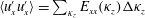 $\langle u_{x}^{\prime }u_{x}^{\prime }\rangle =\sum _{\unicode[STIX]{x1D705}_{z}}E_{xx}(\unicode[STIX]{x1D705}_{z})\unicode[STIX]{x0394}\unicode[STIX]{x1D705}_{z}$
. Similarly, we define a spectral density function for the fluctuating vorticity
$\langle u_{x}^{\prime }u_{x}^{\prime }\rangle =\sum _{\unicode[STIX]{x1D705}_{z}}E_{xx}(\unicode[STIX]{x1D705}_{z})\unicode[STIX]{x0394}\unicode[STIX]{x1D705}_{z}$
. Similarly, we define a spectral density function for the fluctuating vorticity
 $$\begin{eqnarray}\unicode[STIX]{x1D6F7}_{ij}(\unicode[STIX]{x1D705}_{z},x,y,\unicode[STIX]{x1D703})=\frac{1}{\unicode[STIX]{x0394}\unicode[STIX]{x1D705}_{z}}\langle \hat{\unicode[STIX]{x1D714}}_{i}^{\prime }(\unicode[STIX]{x1D705}_{z},x,y,\unicode[STIX]{x1D703})\hat{\unicode[STIX]{x1D714}}_{j}^{^{\prime }\ast }(\unicode[STIX]{x1D705}_{z},x,y,\unicode[STIX]{x1D703})\rangle ,\end{eqnarray}$$
where
 $\hat{\unicode[STIX]{x1D714}}_{i}^{\prime }$
are the Fourier coefficients of the fluctuating vorticity. The spectrum of total enstrophy fluctuations is given by
$\hat{\unicode[STIX]{x1D714}}_{i}^{\prime }$
are the Fourier coefficients of the fluctuating vorticity. The spectrum of total enstrophy fluctuations is given by
 $\unicode[STIX]{x1D6F7}_{{\mathcal{E}}}=\unicode[STIX]{x1D6F7}_{ii}/2$
, where repeated indices are summed. We consider this enstrophy spectrum to study the dissipative scales of motion. Finally, the spectral density for wall-shear-stress fluctuations is given by
$\unicode[STIX]{x1D6F7}_{{\mathcal{E}}}=\unicode[STIX]{x1D6F7}_{ii}/2$
, where repeated indices are summed. We consider this enstrophy spectrum to study the dissipative scales of motion. Finally, the spectral density for wall-shear-stress fluctuations is given by
 $$\begin{eqnarray}T_{ij}(\unicode[STIX]{x1D705}_{z},x,y,\unicode[STIX]{x1D703})=\frac{1}{\unicode[STIX]{x0394}\unicode[STIX]{x1D705}_{z}}\langle \hat{\unicode[STIX]{x1D70F}}_{i}^{\prime }(\unicode[STIX]{x1D705}_{z},x,y,\unicode[STIX]{x1D703})\hat{\unicode[STIX]{x1D70F}}_{j}^{^{\prime }\ast }(\unicode[STIX]{x1D705}_{z},x,y,\unicode[STIX]{x1D703})\rangle ,\end{eqnarray}$$
where
 $\hat{\unicode[STIX]{x1D70F}}_{i}^{\prime }$
are the Fourier coefficients of the fluctuating wall-shear-stress component. We will consider only the spectrum of shear-stress fluctuations that are streamwise tangent to the ripple surface, i.e.
$\hat{\unicode[STIX]{x1D70F}}_{i}^{\prime }$
are the Fourier coefficients of the fluctuating wall-shear-stress component. We will consider only the spectrum of shear-stress fluctuations that are streamwise tangent to the ripple surface, i.e.
 $T_{tt}$
.
$T_{tt}$
.
The extracted spectral densities from our database contained a high noise-to-signal ratio due to limited sampling. In order to enhance the presentation, we have smoothed the data using the SciPy implementation of the Savitzky–Golay filter (Savitzky & Golay Reference Savitzky and Golay1964). In this process, we employed second-order polynomials with a window length of nine samples. The raw spectra are shown in some of the figures for reference.

Figure 23. Premultiplied one-dimensional spectra of streamwise turbulent kinetic energy (
 $u_{x}^{\prime }u_{x}^{\prime }$
) and enstrophy (
$u_{x}^{\prime }u_{x}^{\prime }$
) and enstrophy (
 ${\mathcal{E}}$
) evaluated for spanwise wavelengths along the vortex-core trajectories
${\mathcal{E}}$
) evaluated for spanwise wavelengths along the vortex-core trajectories
 $\boldsymbol{x}_{P}(\unicode[STIX]{x1D703})$
and
$\boldsymbol{x}_{P}(\unicode[STIX]{x1D703})$
and
 $\boldsymbol{x}_{S}(\unicode[STIX]{x1D703})$
, cf. table 5 for the definition of trajectories. (a,c)
$\boldsymbol{x}_{S}(\unicode[STIX]{x1D703})$
, cf. table 5 for the definition of trajectories. (a,c)
 $P$
-vortex, i.e.
$P$
-vortex, i.e.
 $\unicode[STIX]{x1D705}_{z}E_{xx}(\unicode[STIX]{x1D705}_{z},\boldsymbol{x}_{P}(\unicode[STIX]{x1D703}),\unicode[STIX]{x1D703})/U_{0}^{2}$
(contours) and
$\unicode[STIX]{x1D705}_{z}E_{xx}(\unicode[STIX]{x1D705}_{z},\boldsymbol{x}_{P}(\unicode[STIX]{x1D703}),\unicode[STIX]{x1D703})/U_{0}^{2}$
(contours) and
 $\unicode[STIX]{x1D705}_{z}\unicode[STIX]{x1D6F7}_{\unicode[STIX]{x1D700}}(\unicode[STIX]{x1D705}_{z},\boldsymbol{x}_{P}(\unicode[STIX]{x1D703}),\unicode[STIX]{x1D703})/(U_{0}/\unicode[STIX]{x1D702})^{2}$
(shades). (b,d)
$\unicode[STIX]{x1D705}_{z}\unicode[STIX]{x1D6F7}_{\unicode[STIX]{x1D700}}(\unicode[STIX]{x1D705}_{z},\boldsymbol{x}_{P}(\unicode[STIX]{x1D703}),\unicode[STIX]{x1D703})/(U_{0}/\unicode[STIX]{x1D702})^{2}$
(shades). (b,d)
 $S$
-vortex, i.e.
$S$
-vortex, i.e.
 $\unicode[STIX]{x1D705}_{z}E_{xx}(\unicode[STIX]{x1D705}_{z},\boldsymbol{x}_{S}(\unicode[STIX]{x1D703}),\unicode[STIX]{x1D703})/U_{0}^{2}$
(contours) and
$\unicode[STIX]{x1D705}_{z}E_{xx}(\unicode[STIX]{x1D705}_{z},\boldsymbol{x}_{S}(\unicode[STIX]{x1D703}),\unicode[STIX]{x1D703})/U_{0}^{2}$
(contours) and
 $\unicode[STIX]{x1D705}_{z}\unicode[STIX]{x1D6F7}_{\unicode[STIX]{x1D700}}(\unicode[STIX]{x1D705}_{z},\boldsymbol{x}_{S}(\unicode[STIX]{x1D703}),\unicode[STIX]{x1D703})/(U_{0}/\unicode[STIX]{x1D702})^{2}$
(shades). (a,b) Case C1, contour levels are
$\unicode[STIX]{x1D705}_{z}\unicode[STIX]{x1D6F7}_{\unicode[STIX]{x1D700}}(\unicode[STIX]{x1D705}_{z},\boldsymbol{x}_{S}(\unicode[STIX]{x1D703}),\unicode[STIX]{x1D703})/(U_{0}/\unicode[STIX]{x1D702})^{2}$
(shades). (a,b) Case C1, contour levels are
 $0.04(0.04)0.32$
; (c,d) Case C2, contour levels are
$0.04(0.04)0.32$
; (c,d) Case C2, contour levels are
 $0.025(0.025)0.2$
.
$0.025(0.025)0.2$
.
Figure 23 shows the premultiplied spectral densities
 $\unicode[STIX]{x1D705}_{z}E_{xx}$
(lines) and
$\unicode[STIX]{x1D705}_{z}E_{xx}$
(lines) and
 $\unicode[STIX]{x1D705}_{z}\unicode[STIX]{x1D6F7}_{{\mathcal{E}}}$
(shades) along the vortex-core trajectories
$\unicode[STIX]{x1D705}_{z}\unicode[STIX]{x1D6F7}_{{\mathcal{E}}}$
(shades) along the vortex-core trajectories
 $\boldsymbol{x}_{P}(\unicode[STIX]{x1D703})$
and
$\boldsymbol{x}_{P}(\unicode[STIX]{x1D703})$
and
 $\boldsymbol{x}_{S}(\unicode[STIX]{x1D703})$
. A premultiplied spectral density plot shows the energy per
$\boldsymbol{x}_{S}(\unicode[STIX]{x1D703})$
. A premultiplied spectral density plot shows the energy per
 $\log \unicode[STIX]{x1D705}_{z}$
, or
$\log \unicode[STIX]{x1D705}_{z}$
, or
 $\log \unicode[STIX]{x1D706}_{z}$
. To show this, we first write the total energy using continuous variables
$\log \unicode[STIX]{x1D706}_{z}$
. To show this, we first write the total energy using continuous variables
 $\langle u_{x}^{\prime }u_{x}^{\prime }\rangle =\sum E_{xx}\unicode[STIX]{x0394}\unicode[STIX]{x1D705}_{z}\approx \int E_{xx}\,\text{d}\unicode[STIX]{x1D705}_{z}$
. In a log–linear plot with a logarithmic axis of wavenumbers, the integral reads
$\langle u_{x}^{\prime }u_{x}^{\prime }\rangle =\sum E_{xx}\unicode[STIX]{x0394}\unicode[STIX]{x1D705}_{z}\approx \int E_{xx}\,\text{d}\unicode[STIX]{x1D705}_{z}$
. In a log–linear plot with a logarithmic axis of wavenumbers, the integral reads
 $\int E_{xx}\,\text{d}\unicode[STIX]{x1D705}_{z}=\int \unicode[STIX]{x1D705}_{z}E_{xx}\,\text{d}\log \unicode[STIX]{x1D705}_{z}$
, where we have used
$\int E_{xx}\,\text{d}\unicode[STIX]{x1D705}_{z}=\int \unicode[STIX]{x1D705}_{z}E_{xx}\,\text{d}\log \unicode[STIX]{x1D705}_{z}$
, where we have used
 $\text{d}\unicode[STIX]{x1D705}_{z}=\text{d}\log \unicode[STIX]{x1D705}_{z}/\unicode[STIX]{x1D705}_{z}$
. Finally, wavenumbers and wavelengths can be interchanged without modifying the integrand, as
$\text{d}\unicode[STIX]{x1D705}_{z}=\text{d}\log \unicode[STIX]{x1D705}_{z}/\unicode[STIX]{x1D705}_{z}$
. Finally, wavenumbers and wavelengths can be interchanged without modifying the integrand, as
 $\text{d}\log \unicode[STIX]{x1D705}_{z}=-\text{d}\log \unicode[STIX]{x1D706}_{z}$
, i.e.
$\text{d}\log \unicode[STIX]{x1D705}_{z}=-\text{d}\log \unicode[STIX]{x1D706}_{z}$
, i.e.
 $\int _{\unicode[STIX]{x1D705}_{min}}^{\unicode[STIX]{x1D705}_{max}}\unicode[STIX]{x1D705}_{z}E_{xx}\,\text{d}\log \unicode[STIX]{x1D705}_{z}=-\!\int _{\unicode[STIX]{x1D706}_{max}}^{\unicode[STIX]{x1D706}_{min}}\unicode[STIX]{x1D705}_{z}E_{xx}\,\text{d}\log \unicode[STIX]{x1D706}_{z}=\int _{\unicode[STIX]{x1D706}_{min}}^{\unicode[STIX]{x1D706}_{max}}\unicode[STIX]{x1D705}_{z}E_{xx}\,\text{d}\log \unicode[STIX]{x1D706}_{z}$
. In the premultiplied spectrum plots, equal areas indicate equal contributions to energy. Premultiplied spectral density analysis is commonly employed to identify energetic turbulent structures in regions with intense multiscale dynamics, e.g. outer layer of wall-bounded flows (Hutchins & Marusic Reference Hutchins and Marusic2007; Jiménez Reference Jiménez2013).
$\int _{\unicode[STIX]{x1D705}_{min}}^{\unicode[STIX]{x1D705}_{max}}\unicode[STIX]{x1D705}_{z}E_{xx}\,\text{d}\log \unicode[STIX]{x1D705}_{z}=-\!\int _{\unicode[STIX]{x1D706}_{max}}^{\unicode[STIX]{x1D706}_{min}}\unicode[STIX]{x1D705}_{z}E_{xx}\,\text{d}\log \unicode[STIX]{x1D706}_{z}=\int _{\unicode[STIX]{x1D706}_{min}}^{\unicode[STIX]{x1D706}_{max}}\unicode[STIX]{x1D705}_{z}E_{xx}\,\text{d}\log \unicode[STIX]{x1D706}_{z}$
. In the premultiplied spectrum plots, equal areas indicate equal contributions to energy. Premultiplied spectral density analysis is commonly employed to identify energetic turbulent structures in regions with intense multiscale dynamics, e.g. outer layer of wall-bounded flows (Hutchins & Marusic Reference Hutchins and Marusic2007; Jiménez Reference Jiménez2013).
We see in figure 23 that contour lines and shaded contours minimally overlap in C1 (figure 23
a,b), while they share most of the spectrum in C2 (figure 23
c,d). Namely, the dissipative (enstrophy-containing) and energy-containing scales are well separated in C1, as the former occurs on substantially smaller scales. Saffman (Reference Saffman1978) suggested a well-defined separation between the energy-containing range and the dissipative range when the Taylor-microscale Reynolds number exceeds a critical value
 $Re_{T}^{c}\approx 100$
. Our results are consistent with Saffman’s conjecture, as
$Re_{T}^{c}\approx 100$
. Our results are consistent with Saffman’s conjecture, as
 $Re_{T}>Re_{T}^{c}$
along
$Re_{T}>Re_{T}^{c}$
along
 $\boldsymbol{x}_{P}$
and
$\boldsymbol{x}_{P}$
and
 $\boldsymbol{x}_{S}$
in the case of C1, and
$\boldsymbol{x}_{S}$
in the case of C1, and
 $Re_{T}\approx 60$
in the case of C2 (cf. figures 16
e and 16
j). Dimotakis (Reference Dimotakis2000) further showed that many turbulent flows change their dynamics and qualitative behaviour when their Reynolds number is above
$Re_{T}\approx 60$
in the case of C2 (cf. figures 16
e and 16
j). Dimotakis (Reference Dimotakis2000) further showed that many turbulent flows change their dynamics and qualitative behaviour when their Reynolds number is above
 $Re_{T}^{c}$
. He defined this second step of transition (after the breakdown of the laminar state) as the mixing transition, since the flows possess significantly enhanced and more homogeneous mixing properties following this transition. Beyond the mixing transition, general flow properties appear to be only weakly dependent on the Reynolds number, hence the turbulence can be assumed to be fully developed. In this regard, the flow in C1 is in a fully developed post-mixing-transition state. Marked differences in the instantaneous snapshots (figure 20) and big disparity in the enstrophy levels of the cases (cf. e.g. figures 15
b and 15
g) can be attributed to this fact.
$Re_{T}^{c}$
. He defined this second step of transition (after the breakdown of the laminar state) as the mixing transition, since the flows possess significantly enhanced and more homogeneous mixing properties following this transition. Beyond the mixing transition, general flow properties appear to be only weakly dependent on the Reynolds number, hence the turbulence can be assumed to be fully developed. In this regard, the flow in C1 is in a fully developed post-mixing-transition state. Marked differences in the instantaneous snapshots (figure 20) and big disparity in the enstrophy levels of the cases (cf. e.g. figures 15
b and 15
g) can be attributed to this fact.
We now turn to the spectral distribution of the streamwise turbulent kinetic energy along the trajectories of the vortex cores. The peaks in the spectra at each phase are marked with dots in figure 23. It is observed in figure 23(a) that the energy in
 $P$
-vortex cores initially centred around a peak at
$P$
-vortex cores initially centred around a peak at
 $\unicode[STIX]{x1D706}_{z}\approx 0.6\unicode[STIX]{x1D706}$
in Case C1. The energetic centre slowly evolves to
$\unicode[STIX]{x1D706}_{z}\approx 0.6\unicode[STIX]{x1D706}$
in Case C1. The energetic centre slowly evolves to
 $\unicode[STIX]{x1D706}_{z}\approx 0.9\unicode[STIX]{x1D706}$
and remains dominant throughout the remaining lifetime of the vortex. This high concentration of energy in certain wavelengths is the manifestation of a dominant vortex mode. This mode is responsible for breaking down coherent spanwise vortices into intermittent vortex clusters in C1, cf. § 6.1. The wavelengths of the peaks represent the average spanwise spacing for large-scale structures observed in figure 20(a,c,e) and figure 21(b,d). A similar energetic vortex mode is also observed in the
$\unicode[STIX]{x1D706}_{z}\approx 0.9\unicode[STIX]{x1D706}$
and remains dominant throughout the remaining lifetime of the vortex. This high concentration of energy in certain wavelengths is the manifestation of a dominant vortex mode. This mode is responsible for breaking down coherent spanwise vortices into intermittent vortex clusters in C1, cf. § 6.1. The wavelengths of the peaks represent the average spanwise spacing for large-scale structures observed in figure 20(a,c,e) and figure 21(b,d). A similar energetic vortex mode is also observed in the
 $P$
-vortex cores of Case C2, cf. figure 23(c). The growth of the mode in both cases, i.e. the increase of the wavelengths from
$P$
-vortex cores of Case C2, cf. figure 23(c). The growth of the mode in both cases, i.e. the increase of the wavelengths from
 $\unicode[STIX]{x1D706}_{z}\approx 0.6\unicode[STIX]{x1D706}$
to
$\unicode[STIX]{x1D706}_{z}\approx 0.6\unicode[STIX]{x1D706}$
to
 $\unicode[STIX]{x1D706}_{z}\approx 0.9\unicode[STIX]{x1D706}$
, suggests merging of some neighbouring structures during the evolution of the coherent vortex.
$\unicode[STIX]{x1D706}_{z}\approx 0.9\unicode[STIX]{x1D706}$
, suggests merging of some neighbouring structures during the evolution of the coherent vortex.
Figure 23(b,d) shows that the energetic vortex mode is also effective in the
 $S$
-vortices. It becomes increasingly prominent in the spectra when the vortex moves towards the crest in the self-ejection process in the range
$S$
-vortices. It becomes increasingly prominent in the spectra when the vortex moves towards the crest in the self-ejection process in the range
 $12\unicode[STIX]{x03C0}/32\leqslant \unicode[STIX]{x1D703}\leqslant 20\unicode[STIX]{x03C0}/32$
. The energy of the mode reaches a global peak around
$12\unicode[STIX]{x03C0}/32\leqslant \unicode[STIX]{x1D703}\leqslant 20\unicode[STIX]{x03C0}/32$
. The energy of the mode reaches a global peak around
 $\unicode[STIX]{x1D703}=20\unicode[STIX]{x03C0}/32$
, i.e. just before the ejection of the vortex from the crest. We see that after the ejection, the portion of the vortex mode in
$\unicode[STIX]{x1D703}=20\unicode[STIX]{x03C0}/32$
, i.e. just before the ejection of the vortex from the crest. We see that after the ejection, the portion of the vortex mode in
 $S$
-vortex is demolished, and energy concentrates in smaller wavelengths, cf.
$S$
-vortex is demolished, and energy concentrates in smaller wavelengths, cf.
 $\unicode[STIX]{x1D703}>24\unicode[STIX]{x03C0}/32$
in figure 23(b,d). We also note that after ejection from the wall, the enstrophy significantly increases in the
$\unicode[STIX]{x1D703}>24\unicode[STIX]{x03C0}/32$
in figure 23(b,d). We also note that after ejection from the wall, the enstrophy significantly increases in the
 $S$
-vortex core, cf. the rise in the shaded contour levels in figure 23(b,d). This suggests a transition to a more dissipative and less coherent state, under which small-scale motions are promoted.
$S$
-vortex core, cf. the rise in the shaded contour levels in figure 23(b,d). This suggests a transition to a more dissipative and less coherent state, under which small-scale motions are promoted.
The overall dominance of the vortex mode can be elaborated using the cumulative energy contribution of the spectral range related to this mode. Such a cumulative analysis, where a certain range of scales is attributed to a class of turbulent structures, has been previously employed to investigate the prominence of flow structures in turbulent wall-bounded flows, cf. e.g. Guala, Hommema & Adrian (Reference Guala, Hommema and Adrian2006). To this end, the fraction of the fluctuation energy in the wavelengths greater or equal than a selected wavelength
 $\unicode[STIX]{x1D706}_{c}$
is calculated with
$\unicode[STIX]{x1D706}_{c}$
is calculated with
 $$\begin{eqnarray}\unicode[STIX]{x1D6F6}_{ij}(\unicode[STIX]{x1D706}_{c})=\frac{\displaystyle \mathop{\sum }_{\unicode[STIX]{x1D705}_{z}=0}^{\unicode[STIX]{x1D705}_{z}=2\unicode[STIX]{x03C0}/\unicode[STIX]{x1D706}_{c}}E_{ij}(\unicode[STIX]{x1D705}_{z})}{\displaystyle \mathop{\sum }_{\unicode[STIX]{x1D705}_{z}=0}^{\unicode[STIX]{x1D705}_{z}=\unicode[STIX]{x1D705}_{z}^{max}}E_{ij}(\unicode[STIX]{x1D705}_{z})}.\end{eqnarray}$$
We omitted the explicit dependency of
 $E_{ij}$
on
$E_{ij}$
on
 $y,z,\unicode[STIX]{x1D703}$
for brevity. To conduct the analysis, we associate the energy in the long-wavelength range
$y,z,\unicode[STIX]{x1D703}$
for brevity. To conduct the analysis, we associate the energy in the long-wavelength range
 $\unicode[STIX]{x1D706}_{z}\geqslant 0.5\unicode[STIX]{x1D706}$
with the vortex mode. This threshold is demonstrated with vertical lines in figure 23. Figure 24 shows the fraction of the streamwise turbulent kinetic energy in the range
$\unicode[STIX]{x1D706}_{z}\geqslant 0.5\unicode[STIX]{x1D706}$
with the vortex mode. This threshold is demonstrated with vertical lines in figure 23. Figure 24 shows the fraction of the streamwise turbulent kinetic energy in the range
 $\unicode[STIX]{x1D706}_{z}\geqslant 0.5\unicode[STIX]{x1D706}$
, i.e.
$\unicode[STIX]{x1D706}_{z}\geqslant 0.5\unicode[STIX]{x1D706}$
, i.e.
 $\unicode[STIX]{x1D6F6}_{xx}(0.5\unicode[STIX]{x1D706})$
, evaluated along
$\unicode[STIX]{x1D6F6}_{xx}(0.5\unicode[STIX]{x1D706})$
, evaluated along
 $\boldsymbol{x}_{P}(\unicode[STIX]{x1D703})$
and
$\boldsymbol{x}_{P}(\unicode[STIX]{x1D703})$
and
 $\boldsymbol{x}_{S}(\unicode[STIX]{x1D703})$
. We see that the
$\boldsymbol{x}_{S}(\unicode[STIX]{x1D703})$
. We see that the
 $P^{+}$
–
$P^{+}$
–
 $S^{-}$
dipole is unstable to the vortex mode, whose energy grows during the motion of the dipole towards the crest. When the vortices pass the crest at
$S^{-}$
dipole is unstable to the vortex mode, whose energy grows during the motion of the dipole towards the crest. When the vortices pass the crest at
 $x/\unicode[STIX]{x1D702}=6$
, coherent motions related to the vortex mode contain a significant portion of the total streamwise fluctuation energy – approximately
$x/\unicode[STIX]{x1D702}=6$
, coherent motions related to the vortex mode contain a significant portion of the total streamwise fluctuation energy – approximately
 $70\,\%$
in the
$70\,\%$
in the
 $P$
-vortex core, and approximately
$P$
-vortex core, and approximately
 $75\,\%$
in the
$75\,\%$
in the
 $S$
-vortex core. Large-scale dynamics of vortices differs following their ejection from the crest. We have previously seen that
$S$
-vortex core. Large-scale dynamics of vortices differs following their ejection from the crest. We have previously seen that
 $S^{-}$
vortex loses most of the large-scale energy after it passes the crest. This is also clearly seen in figure 24(b), where
$S^{-}$
vortex loses most of the large-scale energy after it passes the crest. This is also clearly seen in figure 24(b), where
 $\unicode[STIX]{x1D6F6}_{xx}(0.5\unicode[STIX]{x1D706})$
decreases rapidly to approximately
$\unicode[STIX]{x1D6F6}_{xx}(0.5\unicode[STIX]{x1D706})$
decreases rapidly to approximately
 $40\,\%$
following
$40\,\%$
following
 $x/\unicode[STIX]{x1D702}>6.5$
. In contrast, the coherent large-scale motions remain active in the primary vortex, and their fractional contributions to the overall energy remain above
$x/\unicode[STIX]{x1D702}>6.5$
. In contrast, the coherent large-scale motions remain active in the primary vortex, and their fractional contributions to the overall energy remain above
 $60\,\%$
. This difference between
$60\,\%$
. This difference between
 $P$
- and
$P$
- and
 $S$
-vortices is likely due to their respective distances to the ripple surface, which seems to dissolve the portion of the vortex mode passing nearby.
$S$
-vortices is likely due to their respective distances to the ripple surface, which seems to dissolve the portion of the vortex mode passing nearby.
Figure 23 showed that preferred spanwise spacings of the three-dimensional structures driven by the energetic vortex mode vary in the range
 $0.6<\unicode[STIX]{x1D706}_{z}/\unicode[STIX]{x1D706}<0.9$
. These values are in the same range with the spanwise spacing of the brick patterns (
$0.6<\unicode[STIX]{x1D706}_{z}/\unicode[STIX]{x1D706}<0.9$
. These values are in the same range with the spanwise spacing of the brick patterns (
 $0.6<\unicode[STIX]{x1D706}_{z}/\unicode[STIX]{x1D706}<1.3$
) observed by Ourmieres & Chaplin (Reference Ourmieres and Chaplin2004) in disturbed-laminar regimes over vortex ripples. Moreover, we have observed in § 6.1 that the arrangement of large-scale structures in Case C1 is also reminiscent of brick patterns. In this regard, the current study provides preliminary evidence for the emergence of these subharmonic flow patterns in fully turbulent regimes.
$0.6<\unicode[STIX]{x1D706}_{z}/\unicode[STIX]{x1D706}<1.3$
) observed by Ourmieres & Chaplin (Reference Ourmieres and Chaplin2004) in disturbed-laminar regimes over vortex ripples. Moreover, we have observed in § 6.1 that the arrangement of large-scale structures in Case C1 is also reminiscent of brick patterns. In this regard, the current study provides preliminary evidence for the emergence of these subharmonic flow patterns in fully turbulent regimes.

Figure 24. The cumulative fraction of the streamwise turbulent kinetic energy in transverse wavelengths
 $\unicode[STIX]{x1D706}_{z}\geqslant 0.5\unicode[STIX]{x1D706}$
, cf. (6.5). (a) Evaluated on
$\unicode[STIX]{x1D706}_{z}\geqslant 0.5\unicode[STIX]{x1D706}$
, cf. (6.5). (a) Evaluated on
 $\boldsymbol{x}_{P}(\unicode[STIX]{x1D703})$
in
$\boldsymbol{x}_{P}(\unicode[STIX]{x1D703})$
in
 $4\unicode[STIX]{x03C0}/32\leqslant \unicode[STIX]{x1D703}\leqslant \unicode[STIX]{x03C0}$
; (b) evaluated on
$4\unicode[STIX]{x03C0}/32\leqslant \unicode[STIX]{x1D703}\leqslant \unicode[STIX]{x03C0}$
; (b) evaluated on
 $\boldsymbol{x}_{S}(\unicode[STIX]{x1D703})$
in
$\boldsymbol{x}_{S}(\unicode[STIX]{x1D703})$
in
 $12\unicode[STIX]{x03C0}/32\leqslant \unicode[STIX]{x1D703}\leqslant \unicode[STIX]{x03C0}$
, cf. table 5 for trajectories
$12\unicode[STIX]{x03C0}/32\leqslant \unicode[STIX]{x1D703}\leqslant \unicode[STIX]{x03C0}$
, cf. table 5 for trajectories
 $\boldsymbol{x}_{P}(\unicode[STIX]{x1D703})$
and
$\boldsymbol{x}_{P}(\unicode[STIX]{x1D703})$
and
 $\boldsymbol{x}_{S}(\unicode[STIX]{x1D703})$
. (○) Case C1; (▫) Case C2. Each data point is separated by
$\boldsymbol{x}_{S}(\unicode[STIX]{x1D703})$
. (○) Case C1; (▫) Case C2. Each data point is separated by
 $\unicode[STIX]{x03C0}/32$
in time, and filled markers indicate every fourth data point.
$\unicode[STIX]{x03C0}/32$
in time, and filled markers indicate every fourth data point.
Canals & Pawlak (Reference Canals and Pawlak2011) also reported dominant large-scale structures on a vortex dipole, which is formed around a single ripple attached to an oscillating tray. These structures were formed by an elliptic instability of the strained vortex cores, and had spanwise spacings in the range
 $2<\unicode[STIX]{x1D706}_{z}/r<5$
, where
$2<\unicode[STIX]{x1D706}_{z}/r<5$
, where
 $r$
is the vortex-core radius. If we assume the radius of the vortex cores in our study is approximately
$r$
is the vortex-core radius. If we assume the radius of the vortex cores in our study is approximately
 $r\approx \unicode[STIX]{x1D702}$
, then there is a good overlap between the observed spanwise spacings in our simulations (
$r\approx \unicode[STIX]{x1D702}$
, then there is a good overlap between the observed spanwise spacings in our simulations (
 $3.6<\unicode[STIX]{x1D706}_{z}/\unicode[STIX]{x1D702}<5.4$
) and in experiments by Canals & Pawlak (Reference Canals and Pawlak2011). Furthermore, we have seen in figure 24 that the vortex mode energy increases during the motion of the dipole towards the crest in the range
$3.6<\unicode[STIX]{x1D706}_{z}/\unicode[STIX]{x1D702}<5.4$
) and in experiments by Canals & Pawlak (Reference Canals and Pawlak2011). Furthermore, we have seen in figure 24 that the vortex mode energy increases during the motion of the dipole towards the crest in the range
 $8\unicode[STIX]{x03C0}/32\leqslant \unicode[STIX]{x1D703}\leqslant 16\unicode[STIX]{x03C0}/32$
. This is the stage where the vortices mutually strain each other to elliptic forms (cf. figures 4
c–e and 5
c–e in § 3). Therefore, we believe that the observed vortex mode is driven by elliptic instabilities of coherent-vortex cores.
$8\unicode[STIX]{x03C0}/32\leqslant \unicode[STIX]{x1D703}\leqslant 16\unicode[STIX]{x03C0}/32$
. This is the stage where the vortices mutually strain each other to elliptic forms (cf. figures 4
c–e and 5
c–e in § 3). Therefore, we believe that the observed vortex mode is driven by elliptic instabilities of coherent-vortex cores.

Figure 25. Premultiplied streamwise turbulent kinetic energy spectra evaluated at the
 $P$
-vortex core (black) and at the
$P$
-vortex core (black) and at the
 $S$
-vortex core (red), and premultiplied wall-shear-stress spectra evaluated at the local wall-shear-stress maximum (green). (a,c)
$S$
-vortex core (red), and premultiplied wall-shear-stress spectra evaluated at the local wall-shear-stress maximum (green). (a,c)
 $\unicode[STIX]{x1D703}=20\unicode[STIX]{x03C0}/32$
; (b,d)
$\unicode[STIX]{x1D703}=20\unicode[STIX]{x03C0}/32$
; (b,d)
 $\unicode[STIX]{x1D703}=31\unicode[STIX]{x03C0}/32$
. (a,b) Case C1; (c,d) Case C2. The thin lines show raw spectra without the Savitzky–Golay filter. The spectra are normalized with the local average values such that areas under the curves are equal to unity. The markers in insets show the respective probing points
$\unicode[STIX]{x1D703}=31\unicode[STIX]{x03C0}/32$
. (a,b) Case C1; (c,d) Case C2. The thin lines show raw spectra without the Savitzky–Golay filter. The spectra are normalized with the local average values such that areas under the curves are equal to unity. The markers in insets show the respective probing points
 $\boldsymbol{x}_{P}$
,
$\boldsymbol{x}_{P}$
,
 $\boldsymbol{x}_{S}$
and
$\boldsymbol{x}_{S}$
and
 $\boldsymbol{x}_{\unicode[STIX]{x1D70F}}$
, where the same colour coding with the lines is employed.
$\boldsymbol{x}_{\unicode[STIX]{x1D70F}}$
, where the same colour coding with the lines is employed.
We have shown in § 6.1 that large-scale momentum structures have strong footprints on the wall. Figure 25 elaborates this by comparing the premultiplied spanwise spectra evaluated at the cores of primary and secondary vortices,
 $\unicode[STIX]{x1D705}_{z}E_{xx}(\boldsymbol{x}_{P})$
,
$\unicode[STIX]{x1D705}_{z}E_{xx}(\boldsymbol{x}_{P})$
,
 $\unicode[STIX]{x1D705}_{z}E_{xx}(\boldsymbol{x}_{S})$
and at the local wall-shear-stress peak,
$\unicode[STIX]{x1D705}_{z}E_{xx}(\boldsymbol{x}_{S})$
and at the local wall-shear-stress peak,
 $\unicode[STIX]{x1D705}_{z}T_{tt}(\boldsymbol{x}_{\unicode[STIX]{x1D70F}})$
, for the phases previously employed in figure 21, i.e.
$\unicode[STIX]{x1D705}_{z}T_{tt}(\boldsymbol{x}_{\unicode[STIX]{x1D70F}})$
, for the phases previously employed in figure 21, i.e.
 $\unicode[STIX]{x1D703}=20\unicode[STIX]{x03C0}/32,31\unicode[STIX]{x03C0}/32$
. All spectra are normalized with local fluctuation levels such that the areas under the curves are equal to unity. It is observed in both cases at
$\unicode[STIX]{x1D703}=20\unicode[STIX]{x03C0}/32,31\unicode[STIX]{x03C0}/32$
. All spectra are normalized with local fluctuation levels such that the areas under the curves are equal to unity. It is observed in both cases at
 $\unicode[STIX]{x1D703}=20\unicode[STIX]{x03C0}/32$
that the vortex mode yields a dominant peak at
$\unicode[STIX]{x1D703}=20\unicode[STIX]{x03C0}/32$
that the vortex mode yields a dominant peak at
 $\unicode[STIX]{x1D706}_{z}=0.9\unicode[STIX]{x1D706}$
in all three spectra, cf. solid vertical lines in figure 25(a,c). There is a second peak with shorter wavelength in the wall-shear-stress spectra, cf. dashed vertical lines in figure 25(a,c). This peak appears to be Reynolds number dependent, and occurs on smaller wavelengths in Case C1. The secondary peak is not observed in the vortex cores, as it is related to the streaky velocity field induced by streamwise vortices near the wall. At
$\unicode[STIX]{x1D706}_{z}=0.9\unicode[STIX]{x1D706}$
in all three spectra, cf. solid vertical lines in figure 25(a,c). There is a second peak with shorter wavelength in the wall-shear-stress spectra, cf. dashed vertical lines in figure 25(a,c). This peak appears to be Reynolds number dependent, and occurs on smaller wavelengths in Case C1. The secondary peak is not observed in the vortex cores, as it is related to the streaky velocity field induced by streamwise vortices near the wall. At
 $\unicode[STIX]{x1D703}=31\unicode[STIX]{x03C0}/32$
, the second peak appears to be absent in
$\unicode[STIX]{x1D703}=31\unicode[STIX]{x03C0}/32$
, the second peak appears to be absent in
 $\unicode[STIX]{x1D705}_{z}T_{tt}(\boldsymbol{x}_{\unicode[STIX]{x1D70F}})$
, cf. figure 25(b,d). The vortex mode, now active only in the
$\unicode[STIX]{x1D705}_{z}T_{tt}(\boldsymbol{x}_{\unicode[STIX]{x1D70F}})$
, cf. figure 25(b,d). The vortex mode, now active only in the
 $P^{+}$
vortex, still influences the wall-shear-stress spectrum at this phase, cf. solid lines at
$P^{+}$
vortex, still influences the wall-shear-stress spectrum at this phase, cf. solid lines at
 $\unicode[STIX]{x1D706}_{z}=0.9\unicode[STIX]{x1D706}$
in figure 25(b,d). The mode is less dominant at this phase, and the peaks are less pronounced. Moreover,
$\unicode[STIX]{x1D706}_{z}=0.9\unicode[STIX]{x1D706}$
in figure 25(b,d). The mode is less dominant at this phase, and the peaks are less pronounced. Moreover,
 $\unicode[STIX]{x1D705}_{z}E_{xx}(\boldsymbol{x}_{S})$
does not contain such a peak, as
$\unicode[STIX]{x1D705}_{z}E_{xx}(\boldsymbol{x}_{S})$
does not contain such a peak, as
 $S^{-}$
vortex has transitioned to a less coherent state after leaving the crest, as previously shown in figures 23(b,d) and 24(b).
$S^{-}$
vortex has transitioned to a less coherent state after leaving the crest, as previously shown in figures 23(b,d) and 24(b).

Figure 26. Premultiplied spectra of tangential wall-shear-stress fluctuations presented as functions of spanwise wavelength scaled with the Stokes length (
 $\unicode[STIX]{x1D6FF}_{s}=\sqrt{2\unicode[STIX]{x1D708}/\unicode[STIX]{x1D714}}$
). The spectra are evaluated at
$\unicode[STIX]{x1D6FF}_{s}=\sqrt{2\unicode[STIX]{x1D708}/\unicode[STIX]{x1D714}}$
). The spectra are evaluated at
 $\boldsymbol{x}_{\unicode[STIX]{x1D70F}}(20\unicode[STIX]{x03C0}/32)$
in (a) and at
$\boldsymbol{x}_{\unicode[STIX]{x1D70F}}(20\unicode[STIX]{x03C0}/32)$
in (a) and at
 $\boldsymbol{x}_{\unicode[STIX]{x1D70F}}(24\unicode[STIX]{x03C0}/32)$
in (b). The dashed lines show
$\boldsymbol{x}_{\unicode[STIX]{x1D70F}}(24\unicode[STIX]{x03C0}/32)$
in (b). The dashed lines show
 $\unicode[STIX]{x1D706}_{z}/\unicode[STIX]{x1D6FF}_{s}=7$
. The thin lines represent the raw spectra.
$\unicode[STIX]{x1D706}_{z}/\unicode[STIX]{x1D6FF}_{s}=7$
. The thin lines represent the raw spectra.
We now turn to the scaling of organized streamwise vortices. A natural length scale to relate the spacing of streamwise vortices is the boundary-layer thickness over the vortex ripple, which is expected to be related to the Stokes length
 $\unicode[STIX]{x1D6FF}_{s}=\sqrt{2\unicode[STIX]{x1D708}/\unicode[STIX]{x1D714}}$
. Figure 26 shows premultiplied wall-shear-stress spectra at
$\unicode[STIX]{x1D6FF}_{s}=\sqrt{2\unicode[STIX]{x1D708}/\unicode[STIX]{x1D714}}$
. Figure 26 shows premultiplied wall-shear-stress spectra at
 $\unicode[STIX]{x1D703}=20\unicode[STIX]{x03C0}/32,24\unicode[STIX]{x03C0}/32$
as functions of wavelengths that are normalized with the Stokes length. We see that the streamwise structures scale well with the Stokes length for the two cases, i.e. the short-wavelength peaks collapse well at
$\unicode[STIX]{x1D703}=20\unicode[STIX]{x03C0}/32,24\unicode[STIX]{x03C0}/32$
as functions of wavelengths that are normalized with the Stokes length. We see that the streamwise structures scale well with the Stokes length for the two cases, i.e. the short-wavelength peaks collapse well at
 $\unicode[STIX]{x1D706}_{z}/\unicode[STIX]{x1D6FF}_{s}\approx 7$
. The same value (
$\unicode[STIX]{x1D706}_{z}/\unicode[STIX]{x1D6FF}_{s}\approx 7$
. The same value (
 $7\unicode[STIX]{x1D6FF}_{s}$
) is also reported in Blondeaux et al. (Reference Blondeaux, Scandura and Vittori2004) for the spanwise spacing of streamwise vortices forming along the upstream side of ripples (cf. figure 9 and its discussion on p. 224 in Blondeaux et al. (Reference Blondeaux, Scandura and Vittori2004)). Although our limited dataset prevents a further elaboration of this result, it is informative to compare this spacing with the one produced by centrifugal instabilities over vortex ripples, as curved ripple walls can promote these instabilities. Using a wide variety of configurations, Ourmieres & Chaplin (Reference Ourmieres and Chaplin2004) analysed these features in disturbed-laminar regimes. They showed that centrifugal instabilities produce spanwise patterns along the vortex columns with a well-defined spacing of
$7\unicode[STIX]{x1D6FF}_{s}$
) is also reported in Blondeaux et al. (Reference Blondeaux, Scandura and Vittori2004) for the spanwise spacing of streamwise vortices forming along the upstream side of ripples (cf. figure 9 and its discussion on p. 224 in Blondeaux et al. (Reference Blondeaux, Scandura and Vittori2004)). Although our limited dataset prevents a further elaboration of this result, it is informative to compare this spacing with the one produced by centrifugal instabilities over vortex ripples, as curved ripple walls can promote these instabilities. Using a wide variety of configurations, Ourmieres & Chaplin (Reference Ourmieres and Chaplin2004) analysed these features in disturbed-laminar regimes. They showed that centrifugal instabilities produce spanwise patterns along the vortex columns with a well-defined spacing of
 $\unicode[STIX]{x1D706}_{z}/\unicode[STIX]{x1D6FF}_{s}\approx \sqrt{2}\unicode[STIX]{x1D706}^{2}/A\unicode[STIX]{x1D702}$
. In this regard, the spacing of the streamwise structures in our DNS experiments is in the same range but slightly smaller, i.e.
$\unicode[STIX]{x1D706}_{z}/\unicode[STIX]{x1D6FF}_{s}\approx \sqrt{2}\unicode[STIX]{x1D706}^{2}/A\unicode[STIX]{x1D702}$
. In this regard, the spacing of the streamwise structures in our DNS experiments is in the same range but slightly smaller, i.e.
 $\unicode[STIX]{x1D706}_{z}/\unicode[STIX]{x1D6FF}_{s}\approx 7\approx \unicode[STIX]{x1D706}^{2}/A\unicode[STIX]{x1D702}$
. These results point towards possible relations between the short spanwise wavelength patterns in disturbed-laminar and turbulent conditions. Exploring these links further may be an interesting future study that can shed light on the origin and scaling of the streamwise structures over vortex ripples.
$\unicode[STIX]{x1D706}_{z}/\unicode[STIX]{x1D6FF}_{s}\approx 7\approx \unicode[STIX]{x1D706}^{2}/A\unicode[STIX]{x1D702}$
. These results point towards possible relations between the short spanwise wavelength patterns in disturbed-laminar and turbulent conditions. Exploring these links further may be an interesting future study that can shed light on the origin and scaling of the streamwise structures over vortex ripples.
7 Conclusions
We have conducted a DNS study to investigate the sinusoidal oscillatory flow over a two-dimensional wavy bottom. The model conditions were selected to mimic wave-driven flow conditions above long crested sand ripples in coastal regions. Two different Reynolds numbers were involved. The higher-
 $Re$
case was found to produce a fully developed turbulent flow in which energy-containing and dissipative motions concentrate at exclusive scales.
$Re$
case was found to produce a fully developed turbulent flow in which energy-containing and dissipative motions concentrate at exclusive scales.
The oscillatory flow is dominated by coherent columnar vortices of two types. A primary lee vortex is formed during the deceleration phase by the separation of the boundary layer at the ripple crest. When this vortex becomes stronger, the gradients in its pressure field give rise to a secondary flow separation, and eventually a secondary vortex forms at the lee of the ripple. With further weakening of the free-stream velocity, the primary and secondary vortices form a counter-rotating vortex dipole, and move towards the crest. They eventually eject themselves over the ripple crest with their mutually induced velocities. At this moment, they create a high-speed jet near the crest with peak velocities reaching twice that of the maximum free-stream velocity. The inclination angle of the ejection showed a Reynolds number dependence. As the boundary layers are thinner in the higher-
 $Re$
case, the secondary separation and succeeding vortex creation are bound to a smaller volume beneath the primary vortex. Consequently, the primary vortex is less repelled away from the ripple, and the resulting ejection angle is more horizontal. This paves the way for more intense wall–vortex interactions in the higher-
$Re$
case, the secondary separation and succeeding vortex creation are bound to a smaller volume beneath the primary vortex. Consequently, the primary vortex is less repelled away from the ripple, and the resulting ejection angle is more horizontal. This paves the way for more intense wall–vortex interactions in the higher-
 $Re$
case.
$Re$
case.
Coherent vortices are the main transport means for turbulent kinetic energy and enstrophy. The boundary layers on the ripple surface are only mildly turbulent in both cases. The main production zones are the free separated layers with intense shear, and the main dissipation regions are the vortex cores and boundary layers. The global turbulence production rate peaks twice over a half-cycle. The first peak occurs close to the start of the deceleration phase, and the second one takes place when the vortices eject themselves over the ripple. This initial peak is weak in the lower-
 $Re$
case, as milder wall–vortex interactions in this case leave quieter flow in the lee of the ripples for the subsequent vortex-formation stage. The turbulent dissipation is most intense during the formation of coherent vortices.
$Re$
case, as milder wall–vortex interactions in this case leave quieter flow in the lee of the ripples for the subsequent vortex-formation stage. The turbulent dissipation is most intense during the formation of coherent vortices.
The structural characteristics of coherent vortices are investigated by evaluating their statistics along their path and by visualizing their instantaneous regions with high enstrophy. In the beginning of their lives, coherent vortices keep their spanwise coherence, and are in the form of turbulent vortex clouds that fill the entire spanwise extent of the computational domain. A large-scale vortex mode with transverse wavelengths in the range
 $0.6<\unicode[STIX]{x1D706}_{z}/\unicode[STIX]{x1D706}<0.9$
develops along the vortex column when the vortex dipole moves towards the ripple crest in the ejection process. At this phase, the vortex cores are strained by mutual induction, and vortices become more elliptic. Therefore, this vortex mode is possibly a result of an elliptic instability occurring on the vortex dipole, which was previously observed by Canals & Pawlak (Reference Canals and Pawlak2011) in different oscillatory flow settings. Following their detachment from the ripple, the vortices in the higher-
$0.6<\unicode[STIX]{x1D706}_{z}/\unicode[STIX]{x1D706}<0.9$
develops along the vortex column when the vortex dipole moves towards the ripple crest in the ejection process. At this phase, the vortex cores are strained by mutual induction, and vortices become more elliptic. Therefore, this vortex mode is possibly a result of an elliptic instability occurring on the vortex dipole, which was previously observed by Canals & Pawlak (Reference Canals and Pawlak2011) in different oscillatory flow settings. Following their detachment from the ripple, the vortices in the higher-
 $Re$
case begin to lose their spanwise coherence due to the large-scale vortex mode, and develop an external intermittency along the transverse direction. Consequently, they break down into turbulent vortex clusters whose streamwise arrangement is reminiscent of a brick pattern. The breakdown of spanwise coherence and resulting subharmonic vortex patterns are not observed in the lower-
$Re$
case begin to lose their spanwise coherence due to the large-scale vortex mode, and develop an external intermittency along the transverse direction. Consequently, they break down into turbulent vortex clusters whose streamwise arrangement is reminiscent of a brick pattern. The breakdown of spanwise coherence and resulting subharmonic vortex patterns are not observed in the lower-
 $Re$
case.
$Re$
case.
Furthermore, we have observed secondary structures near to the wall in the form of elongated streamwise vortices, which become more evident during the vortex-ejection stage. These highly anisotropic structures have shorter spanwise spacing. The spectral peaks related to these structures are observed to collapse well at
 $\unicode[STIX]{x1D706}_{z}/\unicode[STIX]{x1D6FF}_{s}\approx 7$
when scaled with the Stokes length.
$\unicode[STIX]{x1D706}_{z}/\unicode[STIX]{x1D6FF}_{s}\approx 7$
when scaled with the Stokes length.
Coherent spanwise vortices have been found to have strong footprints in the near-wall region. During their formation, the primary vortex induces a wall shear in a reverse direction to the free-stream velocity. This wall shear becomes more pronounced when the primary and secondary vortices accelerate towards the crest, and produce the high-speed wall jet. This is the phase when the highest values in the local phase-averaged wall shear stress are observed. Moreover, the coherent vortices also yield strong spanwise inhomogeneity in the wall shear stress as they evolve. In the ejection stage, both large-scale structures driven by the vortex mode and streamwise-vortex structures impose strong fluctuations on the ripple surface. This creates a bimodal premultiplied energy spectrum with two distinctive peaks for wall-shear-stress fluctuations. When decaying coherent vortices arrive at the neighbouring ripple towards the end of the free-stream acceleration, their wall-attached portions sweep the ripple surface and dramatically increase the wall shear stress in their convection direction. This leads to highly skewed probability density functions with long tails for the local wall shear stresses in the contact areas.
The findings in this study provide important implications for the breakdown of long crested sand ripples into three-dimensional forms. Large-scale three-dimensional patterns along the transverse vortex columns could produce inhomogeneous sediment suspension and deposition processes. Furthermore, spanwise variations in the wall shear stress can possibly lead inhomogeneous near-surface sediment motions. In this regard, further knowledge about the origin and scaling behaviour of the observed three-dimensional instabilities can be of key practical importance. Experimentation in a wider parameter space is necessary to gain these insights.
Acknowledgements
The authors gratefully acknowledge financial support from the Tier-1 research project funded by the Ministry of Education of Singapore (WBS:R-302-000-126-112). The computational work for this article was fully performed on resources of the National Supercomputing Centre, Singapore (https://www.nscc.sg).
Appendix A. Spectral assessment of the spatial resolution
In this appendix, we further assess the resolution of the dissipative motions using one-dimensional spectra in the homogenous spanwise direction. This spectral analysis tests the spanwise resolution. As dissipative motions are essentially isotropic, and the largest grid spacings in Kolmogorov units have similar values in the
 $x$
–
$x$
–
 $y$
plane and the in
$y$
plane and the in
 $z$
direction (compare the largest values in figure 3
d,e in § 2.3), the results are also instructive for the spatial resolution in the
$z$
direction (compare the largest values in figure 3
d,e in § 2.3), the results are also instructive for the spatial resolution in the
 $x$
–
$x$
–
 $y$
plane.
$y$
plane.
We start with proving the spectra for Kolmogorov’s laws (Kolmogorov Reference Kolmogorov1941), assuming they are applicable in the energetic locations of our flows. We have seen in § 5 that turbulent kinetic energy concentrates in the core of coherent vortices
 $P$
and
$P$
and
 $S$
, on which the trajectories
$S$
, on which the trajectories
 $\boldsymbol{x}_{P}$
and
$\boldsymbol{x}_{P}$
and
 $\boldsymbol{x}_{S}$
are defined. Figure 27 shows the spanwise energy spectra of streamwise velocity fluctuations evaluated at
$\boldsymbol{x}_{S}$
are defined. Figure 27 shows the spanwise energy spectra of streamwise velocity fluctuations evaluated at
 $\boldsymbol{x}_{P}$
and
$\boldsymbol{x}_{P}$
and
 $\boldsymbol{x}_{S}$
at several representative phases with high turbulent kinetic energy. The spectra are presented in Kolmogorov units, i.e.
$\boldsymbol{x}_{S}$
at several representative phases with high turbulent kinetic energy. The spectra are presented in Kolmogorov units, i.e.
 $\unicode[STIX]{x1D706}_{z}/l_{\unicode[STIX]{x1D702}}$
, and are normalized by
$\unicode[STIX]{x1D706}_{z}/l_{\unicode[STIX]{x1D702}}$
, and are normalized by
 $(\unicode[STIX]{x1D700}\unicode[STIX]{x1D708}^{5})^{1/4}$
such that all lines should collapse on the universal Kolmogorov spectrum in the highest wavenumbers, i.e. in the dissipative range. Pope (Reference Pope2000) presented such a collapse for
$(\unicode[STIX]{x1D700}\unicode[STIX]{x1D708}^{5})^{1/4}$
such that all lines should collapse on the universal Kolmogorov spectrum in the highest wavenumbers, i.e. in the dissipative range. Pope (Reference Pope2000) presented such a collapse for
 $\unicode[STIX]{x1D705}_{x}l_{\unicode[STIX]{x1D702}}>0.1$
using the streamwise spectra of many different types of turbulent flows. We see in figure 27(a,b) that all spectra lie on a single curve for
$\unicode[STIX]{x1D705}_{x}l_{\unicode[STIX]{x1D702}}>0.1$
using the streamwise spectra of many different types of turbulent flows. We see in figure 27(a,b) that all spectra lie on a single curve for
 $\unicode[STIX]{x1D705}_{z}l_{\unicode[STIX]{x1D702}}>0.1$
also in our simulations, which shows that dissipative motions are well resolved. In the inertial range, the Kolmogorov spectrum follows the -5/3 power law (Pope Reference Pope2000)
$\unicode[STIX]{x1D705}_{z}l_{\unicode[STIX]{x1D702}}>0.1$
also in our simulations, which shows that dissipative motions are well resolved. In the inertial range, the Kolmogorov spectrum follows the -5/3 power law (Pope Reference Pope2000)
 $$\begin{eqnarray}\frac{E_{xx}(\unicode[STIX]{x1D705}_{z})}{(\unicode[STIX]{x1D700}\unicode[STIX]{x1D708}^{5})^{1/4}}=\frac{4}{3}{\mathcal{C}}_{k}(\unicode[STIX]{x1D705}_{z}l_{\unicode[STIX]{x1D702}})^{-5/3},\end{eqnarray}$$
where
 ${\mathcal{C}}_{k}=0.53$
is the universal Kolmogorov constant (Sreenivasan Reference Sreenivasan1995), and the factor
${\mathcal{C}}_{k}=0.53$
is the universal Kolmogorov constant (Sreenivasan Reference Sreenivasan1995), and the factor
 $4/3$
is added for using the transverse velocity spectra. The dashed lines in figure 27(a,b) represents the power law. We see that
$4/3$
is added for using the transverse velocity spectra. The dashed lines in figure 27(a,b) represents the power law. We see that
 $-5/3$
power law is applicable at the coherent-vortex cores of both cases, and the spectra follows the dashed line in the inertial range starting from
$-5/3$
power law is applicable at the coherent-vortex cores of both cases, and the spectra follows the dashed line in the inertial range starting from
 $\unicode[STIX]{x1D705}_{z}l_{\unicode[STIX]{x1D702}}<0.1$
. The inertial range extends to lower wavenumbers in C1 due to higher Reynolds number in this case.
$\unicode[STIX]{x1D705}_{z}l_{\unicode[STIX]{x1D702}}<0.1$
. The inertial range extends to lower wavenumbers in C1 due to higher Reynolds number in this case.

Figure 27. Spanwise energy spectra of streamwise-velocity fluctuations evaluated at the coherent-vortex cores
 $\boldsymbol{x}_{P}$
and
$\boldsymbol{x}_{P}$
and
 $\boldsymbol{x}_{S}$
and presented as functions of the spanwise wavenumber
$\boldsymbol{x}_{S}$
and presented as functions of the spanwise wavenumber
 $\unicode[STIX]{x1D705}_{z}$
in local Kolmogorov units (
$\unicode[STIX]{x1D705}_{z}$
in local Kolmogorov units (
 $l_{\unicode[STIX]{x1D702}}=(\unicode[STIX]{x1D708}^{3}/\unicode[STIX]{x1D700})^{1/4}$
).
$l_{\unicode[STIX]{x1D702}}=(\unicode[STIX]{x1D708}^{3}/\unicode[STIX]{x1D700})^{1/4}$
).

Figure 28. One-dimensional premultiplied enstrophy spectra evaluated at the coherent-vortex cores
 $\boldsymbol{x}_{P}$
and
$\boldsymbol{x}_{P}$
and
 $\boldsymbol{x}_{S}$
and presented as functions of the spanwise wavenumber
$\boldsymbol{x}_{S}$
and presented as functions of the spanwise wavenumber
 $\unicode[STIX]{x1D705}_{z}$
in local Kolmogorov units (
$\unicode[STIX]{x1D705}_{z}$
in local Kolmogorov units (
 $l_{\unicode[STIX]{x1D702}}=(\unicode[STIX]{x1D708}^{3}/\unicode[STIX]{x1D700})^{1/4}$
). The vertical lines show
$l_{\unicode[STIX]{x1D702}}=(\unicode[STIX]{x1D708}^{3}/\unicode[STIX]{x1D700})^{1/4}$
). The vertical lines show
 $\unicode[STIX]{x1D705}_{z}l_{\unicode[STIX]{x1D702}}=2\unicode[STIX]{x03C0}/40$
.
$\unicode[STIX]{x1D705}_{z}l_{\unicode[STIX]{x1D702}}=2\unicode[STIX]{x03C0}/40$
.
Figure 28 shows the premultiplied enstrophy spectra evaluated at the coherent-vortex cores at the same phases with figure 27. For brevity, only results for C1 are presented. We see that vorticity concentrates around
 $\unicode[STIX]{x1D705}_{z}l_{\unicode[STIX]{x1D702}}\approx 2\unicode[STIX]{x03C0}/40$
, and all curves collapse in the dissipation range, i.e.
$\unicode[STIX]{x1D705}_{z}l_{\unicode[STIX]{x1D702}}\approx 2\unicode[STIX]{x03C0}/40$
, and all curves collapse in the dissipation range, i.e.
 $\unicode[STIX]{x1D705}_{z}l_{\unicode[STIX]{x1D702}}>0.1$
. The peak at
$\unicode[STIX]{x1D705}_{z}l_{\unicode[STIX]{x1D702}}>0.1$
. The peak at
 $\unicode[STIX]{x1D705}_{z}l_{\unicode[STIX]{x1D702}}\approx 2\unicode[STIX]{x03C0}/40$
appears to be universal for small-scale quantities such as vorticity or strain rate at sufficiently high Reynolds numbers, e.g. Jiménez (Reference Jiménez2013) also showed a peaking of the dissipation spectra around
$\unicode[STIX]{x1D705}_{z}l_{\unicode[STIX]{x1D702}}\approx 2\unicode[STIX]{x03C0}/40$
appears to be universal for small-scale quantities such as vorticity or strain rate at sufficiently high Reynolds numbers, e.g. Jiménez (Reference Jiménez2013) also showed a peaking of the dissipation spectra around
 $\unicode[STIX]{x1D705}_{z}l_{\unicode[STIX]{x1D702}}\approx 2\unicode[STIX]{x03C0}/40$
in the logarithmic layer of a wall-bounded flow. Figure 28 also shows that smallest scales of the flow are well resolved in our DNS experiments. There are no noticeable aliasing errors due to underresolution in
$\unicode[STIX]{x1D705}_{z}l_{\unicode[STIX]{x1D702}}\approx 2\unicode[STIX]{x03C0}/40$
in the logarithmic layer of a wall-bounded flow. Figure 28 also shows that smallest scales of the flow are well resolved in our DNS experiments. There are no noticeable aliasing errors due to underresolution in
 $S$
-vortex cores, cf. figure 28(b). We observe only a minor artificial rise due to aliasing in highest wavenumbers at
$S$
-vortex cores, cf. figure 28(b). We observe only a minor artificial rise due to aliasing in highest wavenumbers at
 $(\boldsymbol{x}_{P}(4\unicode[STIX]{x03C0}/32),4\unicode[STIX]{x03C0}/32)$
, cf. the blue line in
$(\boldsymbol{x}_{P}(4\unicode[STIX]{x03C0}/32),4\unicode[STIX]{x03C0}/32)$
, cf. the blue line in
 $\unicode[STIX]{x1D705}_{z}l_{\unicode[STIX]{x1D702}}\geqslant 1$
in figure 28(a). In their DNS study of channel flow, Del Álamo et al. (Reference Del Álamo, Jimenez, Zandonade and Moser2006) calculated the percentage of enstrophy residing in the aliased wavenumber range and found values in the range 2–3 %. We did a similar calculation for the spectra at
$\unicode[STIX]{x1D705}_{z}l_{\unicode[STIX]{x1D702}}\geqslant 1$
in figure 28(a). In their DNS study of channel flow, Del Álamo et al. (Reference Del Álamo, Jimenez, Zandonade and Moser2006) calculated the percentage of enstrophy residing in the aliased wavenumber range and found values in the range 2–3 %. We did a similar calculation for the spectra at
 $(\boldsymbol{x}_{P}(4\unicode[STIX]{x03C0}/32),4\unicode[STIX]{x03C0}/32)$
and found that the enstrophy residing in the aliased range (
$(\boldsymbol{x}_{P}(4\unicode[STIX]{x03C0}/32),4\unicode[STIX]{x03C0}/32)$
and found that the enstrophy residing in the aliased range (
 $\unicode[STIX]{x1D705}_{z}l_{\unicode[STIX]{x1D702}}\geqslant 1$
) is less than
$\unicode[STIX]{x1D705}_{z}l_{\unicode[STIX]{x1D702}}\geqslant 1$
) is less than
 $0.2\,\%$
of the total enstrophy
$0.2\,\%$
of the total enstrophy
 ${\mathcal{E}}(\boldsymbol{x}_{P}(4\unicode[STIX]{x03C0}/32),4\unicode[STIX]{x03C0}/32)$
.
${\mathcal{E}}(\boldsymbol{x}_{P}(4\unicode[STIX]{x03C0}/32),4\unicode[STIX]{x03C0}/32)$
.
Appendix B. Analysis of the computational domain size
In this section, we assess the computational domain lengths in the spanwise and vertical directions. In order to validate the spanwise extent of the domain, the two-point correlation function in the spanwise direction, i.e.
 $$\begin{eqnarray}{\mathcal{R}}_{ij}(\unicode[STIX]{x0394}z,x,y,\unicode[STIX]{x1D703})=\frac{\langle u_{i}^{\prime }(x,y,z,\unicode[STIX]{x1D703})u_{j}^{\prime }(x,y,z+\unicode[STIX]{x0394}z,\unicode[STIX]{x1D703})\rangle }{\langle u_{i}^{\prime }(x,y,z+\unicode[STIX]{x0394}z,\unicode[STIX]{x1D703})^{2}\rangle ^{1/2}\langle u_{j}^{\prime }(x,y,z,\unicode[STIX]{x1D703})^{2}\rangle ^{1/2}},\end{eqnarray}$$
is employed. Figure 29 shows the spanwise correlations of streamwise velocity fluctuations at the coherent-vortex cores of Case C1 (similar results are applicable to C2). Mahesh & Moin (Reference Mahesh and Moin1998) suggests two-point correlation functions should decay completely within the half of the length of the domain, in order to prevent the interference of periodic boundaries with the largest scales of the flow. We see in figures that the spanwise domain length satisfies this condition. The correlation function decays to negligible values for
 $|\unicode[STIX]{x0394}z|>6\unicode[STIX]{x1D702}(=\unicode[STIX]{x1D706})$
with somewhat more noise beyond
$|\unicode[STIX]{x0394}z|>6\unicode[STIX]{x1D702}(=\unicode[STIX]{x1D706})$
with somewhat more noise beyond
 $|\unicode[STIX]{x0394}z|>6\unicode[STIX]{x1D702}$
in the case of
$|\unicode[STIX]{x0394}z|>6\unicode[STIX]{x1D702}$
in the case of
 $P$
-vortex, cf. figure 29(a).
$P$
-vortex, cf. figure 29(a).

Figure 29. Spanwise autocorrelations of streamwise velocity evaluated at the coherent-vortex cores
 $\boldsymbol{x}_{P}$
and
$\boldsymbol{x}_{P}$
and
 $\boldsymbol{x}_{S}$
in Case C1.
$\boldsymbol{x}_{S}$
in Case C1.

Figure 30. Horizontally averaged streamwise velocity (a) and turbulent kinetic energy (b). (–
 $\times$
):
$\times$
):
 $\unicode[STIX]{x1D703}=0$
; (–▫):
$\unicode[STIX]{x1D703}=0$
; (–▫):
 $\unicode[STIX]{x1D703}=8\unicode[STIX]{x03C0}/32$
; (–○):
$\unicode[STIX]{x1D703}=8\unicode[STIX]{x03C0}/32$
; (–○):
 $\unicode[STIX]{x1D703}=16\unicode[STIX]{x03C0}/32$
; (–
$\unicode[STIX]{x1D703}=16\unicode[STIX]{x03C0}/32$
; (–
 $+$
):
$+$
):
 $\unicode[STIX]{x1D703}=24\unicode[STIX]{x03C0}/32$
. Dashed lines in (a) show the value of the free-stream velocity (
$\unicode[STIX]{x1D703}=24\unicode[STIX]{x03C0}/32$
. Dashed lines in (a) show the value of the free-stream velocity (
 $u_{0}(\unicode[STIX]{x1D703})$
) at respective phases.
$u_{0}(\unicode[STIX]{x1D703})$
) at respective phases.
We now turn to the verification of the extent of the vertical domain. For this purpose, we investigate horizontally averaged fields, which are defined as
 $$\begin{eqnarray}\langle \widetilde{\widetilde{\boldsymbol{u}}}\rangle (y,\unicode[STIX]{x1D703})=\frac{1}{\unicode[STIX]{x1D706}}\int _{0}^{\unicode[STIX]{x1D706}}\langle \boldsymbol{u}\rangle (x,y,\unicode[STIX]{x1D703})\,\text{d}x.\end{eqnarray}$$
Figure 30 shows the horizontally averaged streamwise velocity and TKE at several phases in the half-cycle of Case C1. In the free-stream, streamwise velocity should return to irrotational velocity
 $u_{0}$
(cf. (2.4)) and TKE should vanish. We see in figures that these conditions are satisfied for
$u_{0}$
(cf. (2.4)) and TKE should vanish. We see in figures that these conditions are satisfied for
 $y>6\unicode[STIX]{x1D702}$
. Therefore, we conclude that the vertical extent of our computational domain is sufficiently large to allow free-stream conditions away from the bottom.
$y>6\unicode[STIX]{x1D702}$
. Therefore, we conclude that the vertical extent of our computational domain is sufficiently large to allow free-stream conditions away from the bottom.
Appendix C. Comparisons to experimental data
Although there are quite a few experimental studies on oscillatory flow over rippled beds, an equivalent experiment to Cases C1 and C2 has not yet been conducted. Laboratory flows are usually at higher Reynolds numbers than attained in this work and
 $K_{C}$
number and ripple geometries also vary. Despite this limitation, we can examine some common flow features using experimental data with similar configurations. To this end, we consider an experiment by du Toit & Sleath (Reference du Toit and Sleath1981) (TS81 henceforth), which was conducted in an oscillating water tunnel using self-formed ripples. The flow parameters in this experiment are
$K_{C}$
number and ripple geometries also vary. Despite this limitation, we can examine some common flow features using experimental data with similar configurations. To this end, we consider an experiment by du Toit & Sleath (Reference du Toit and Sleath1981) (TS81 henceforth), which was conducted in an oscillating water tunnel using self-formed ripples. The flow parameters in this experiment are
 $Re=21\,617$
and
$Re=21\,617$
and
 $K_{C}=4.46$
. The ripple steepness is the same as our cases (
$K_{C}=4.46$
. The ripple steepness is the same as our cases (
 $s\approx 0.17$
), and the ripple profile is shown by the solid line in figure 31. This profile is slightly sharper towards the crest than the one considered in this work (given by the dashed line in figure 31). Only Case C1 will be considered in the comparison, as it has a closer Reynolds number to the selected experiment.
$s\approx 0.17$
), and the ripple profile is shown by the solid line in figure 31. This profile is slightly sharper towards the crest than the one considered in this work (given by the dashed line in figure 31). Only Case C1 will be considered in the comparison, as it has a closer Reynolds number to the selected experiment.

Figure 31. Comparison of the ripple profiles considered in this work (dashed line) and in du Toit & Sleath (Reference du Toit and Sleath1981) (solid line).
Figure 32 shows the intra-period variations of phase-averaged streamwise velocity and streamwise turbulent intensity at two selected points. The experimental data are digitized from figures 15 and 18 in TS81. The first probing point is slightly above the ripple crest at
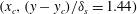 $(x_{c},(y-y_{c})/\unicode[STIX]{x1D6FF}_{s}=1.44)$
and the second point is located above the ripple trough close to crest level at
$(x_{c},(y-y_{c})/\unicode[STIX]{x1D6FF}_{s}=1.44)$
and the second point is located above the ripple trough close to crest level at
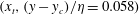 $(x_{t},(y-y_{c})/\unicode[STIX]{x1D702}=0.058)$
, where subscripts
$(x_{t},(y-y_{c})/\unicode[STIX]{x1D702}=0.058)$
, where subscripts
 $c$
and
$c$
and
 $t$
refer to the coordinates of the ripple crest and the ripple trough. The variations in the respective half-cycles of the experimental data are not the mirror image of each other due to some experimental errors.
$t$
refer to the coordinates of the ripple crest and the ripple trough. The variations in the respective half-cycles of the experimental data are not the mirror image of each other due to some experimental errors.
We see in figure 32(a) that the mean streamwise velocity over the ripple crest agrees well with the experimental data within the margin of experimental errors. The peaks in velocity occur when the coherent vortices are washed over the crest at
 $\unicode[STIX]{x1D703}\approx -8/32,24/32\unicode[STIX]{x03C0}$
and when the free-stream velocity has maximum magnitude at
$\unicode[STIX]{x1D703}\approx -8/32,24/32\unicode[STIX]{x03C0}$
and when the free-stream velocity has maximum magnitude at
 $\unicode[STIX]{x1D703}=0,\unicode[STIX]{x03C0}$
. Turbulent intensity peaks during the vortex ejection at
$\unicode[STIX]{x1D703}=0,\unicode[STIX]{x03C0}$
. Turbulent intensity peaks during the vortex ejection at
 $\unicode[STIX]{x1D703}\approx -8/32,24/32\unicode[STIX]{x03C0}$
, and the magnitude and phase of this peak match well. The turbulent intensity between
$\unicode[STIX]{x1D703}\approx -8/32,24/32\unicode[STIX]{x03C0}$
, and the magnitude and phase of this peak match well. The turbulent intensity between
 $-\unicode[STIX]{x03C0}\leqslant \unicode[STIX]{x1D703}\leqslant -24/32\unicode[STIX]{x03C0}$
(
$-\unicode[STIX]{x03C0}\leqslant \unicode[STIX]{x1D703}\leqslant -24/32\unicode[STIX]{x03C0}$
(
 $0\leqslant \unicode[STIX]{x1D703}\leqslant 8/32\unicode[STIX]{x03C0}$
) is higher in TS81.
$0\leqslant \unicode[STIX]{x1D703}\leqslant 8/32\unicode[STIX]{x03C0}$
) is higher in TS81.
Figure 32(b) shows the variations at the point located over the ripple trough. It is observed that the maximum amplitude of the streamwise velocity is approximately
 $U_{0}$
at this location for both Case C1 and TS81. This peak in the velocity occurs when the coherent vortices pass over the ripple trough. This event takes place at
$U_{0}$
at this location for both Case C1 and TS81. This peak in the velocity occurs when the coherent vortices pass over the ripple trough. This event takes place at
 $\unicode[STIX]{x1D703}\approx -4/32,28/32\unicode[STIX]{x03C0}$
in C1 – approximately
$\unicode[STIX]{x1D703}\approx -4/32,28/32\unicode[STIX]{x03C0}$
in C1 – approximately
 $\unicode[STIX]{x1D703}\approx 2/32$
earlier than TS81. A similar delay applies to turbulence intensities, which peak also during the passage of the vortex. This minor phase difference is likely related to the difference in
$\unicode[STIX]{x1D703}\approx 2/32$
earlier than TS81. A similar delay applies to turbulence intensities, which peak also during the passage of the vortex. This minor phase difference is likely related to the difference in
 $K_{C}$
number, which is slightly lower in TS81 (
$K_{C}$
number, which is slightly lower in TS81 (
 $K_{C}=4.46$
) than C1 (
$K_{C}=4.46$
) than C1 (
 $K_{C}=5.24$
), hence the vortex passage corresponds to a later phase.
$K_{C}=5.24$
), hence the vortex passage corresponds to a later phase.

Figure 32. Intra-period variations of phase-averaged streamwise velocity and turbulent intensity over the crest at
 $(x_{c},(y-y_{c})/\unicode[STIX]{x1D6FF}_{s}=1.44)$
(a) and over the trough at
$(x_{c},(y-y_{c})/\unicode[STIX]{x1D6FF}_{s}=1.44)$
(a) and over the trough at
 $(x_{t},(y-y_{c})/\unicode[STIX]{x1D702}=0.058)$
(b), where subscripts
$(x_{t},(y-y_{c})/\unicode[STIX]{x1D702}=0.058)$
(b), where subscripts
 $c$
and
$c$
and
 $t$
refer to the coordinates of the crest and trough, respectively. (
$t$
refer to the coordinates of the crest and trough, respectively. (
 $\times$
):
$\times$
):
 $\langle u_{x}\rangle /U_{0}$
, Case C1; (——):
$\langle u_{x}\rangle /U_{0}$
, Case C1; (——):
 $\langle u_{x}\rangle /U_{0}$
digitized from figure 15 in du Toit & Sleath (Reference du Toit and Sleath1981); (○):
$\langle u_{x}\rangle /U_{0}$
digitized from figure 15 in du Toit & Sleath (Reference du Toit and Sleath1981); (○):
 $\langle u_{x}^{\prime 2}\rangle ^{1/2}/U_{0}$
, Case C1; (
$\langle u_{x}^{\prime 2}\rangle ^{1/2}/U_{0}$
, Case C1; (
 $\cdots$
):
$\cdots$
):
 $\langle u_{x}^{\prime 2}\rangle ^{1/2}/U_{0}$
digitized from figure 18 in du Toit & Sleath (Reference du Toit and Sleath1981).
$\langle u_{x}^{\prime 2}\rangle ^{1/2}/U_{0}$
digitized from figure 18 in du Toit & Sleath (Reference du Toit and Sleath1981).