


1 Introduction
The dynamo instability caused by the motion of conducting fluids is the main source of magnetic-field generation in astrophysical objects such as planets, stars, the interstellar medium and galaxies. In many cases these objects are rotating, rendering the flow strongly anisotropic (Pedlosky Reference Pedlosky1987; Izakov Reference Izakov2013). The Coriolis force, caused by rotation, suppresses the variations along the axis of rotation, leading the flows to become to some extent two-dimensionalized and dependent on only two spacial coordinates, although in some cases retaining all three velocity components, depending on the boundary conditions. This result was first shown in Hough (Reference Hough1897) for linear perturbations and proven in more detail in Taylor (Reference Taylor1917) and Proudman (Reference Proudman1916). The tendency for rotating flows to become two-dimensionalized and the implications of this have been further examined in theoretical investigations (Hopfinger & van Heijst Reference Hopfinger and van Heijst1993; Waleffe Reference Waleffe1993; Scott Reference Scott2014), numerical simulations (Hossain Reference Hossain1994; Yeung & Zhou Reference Yeung and Zhou1998; Smith & Waleffe Reference Smith and Waleffe1999; Chen et al.
Reference Chen, Chen, Eyink and Holm2005; Thiele & Müller Reference Thiele and Müller2009; Mininni & Pouquet Reference Mininni and Pouquet2010; Yoshimatsu, Midorikawa & Kaneda Reference Yoshimatsu, Midorikawa and Kaneda2011; Sen et al.
Reference Sen, Mininni, Rosenberg and Pouquet2012; Deusebio et al.
Reference Deusebio, Boffetta, Lindborg and Musacchio2014; Alexakis Reference Alexakis2015) and laboratory experiments (Sugihara, Migita & Honji Reference Sugihara, Migita and Honji2005; Staplehurst, Davidson & Dalziel Reference Staplehurst, Davidson and Dalziel2008; van Bokhoven et al.
Reference van Bokhoven, Clercx, van Heijst and Trieling2009; Yarom, Vardi & Sharon Reference Yarom, Vardi and Sharon2013; Campagne et al.
Reference Campagne, Gallet, Moisy and Cortet2014; Gallet et al.
Reference Gallet, Campagne, Cortet and Moisy2014). The extent of this two-dimensionalization depends on the rotation rate and is subject to current investigation (Nazarenko & Schekochihin Reference Nazarenko and Schekochihin2011; Baqui & Davidson Reference Baqui and Davidson2015). Recently, theoretical work has shown that the flow becomes exactly two-dimensional (2-D) for free-slip or periodic boundary conditions provided that the rotation is above a critical value (Gallet Reference Gallet2015). This allows one to consider the large-rotation limit which leads to a flow
 $(u(x,y,t),v(x,y,t),w(x,y,t))$
that is independent of the coordinate along the axis of rotation (from here on taken as the
$(u(x,y,t),v(x,y,t),w(x,y,t))$
that is independent of the coordinate along the axis of rotation (from here on taken as the
 $z$
-direction). These flows are referred to in the literature as ‘two-and-a-half’-dimensional (2.5-D) flows or the
$z$
-direction). These flows are referred to in the literature as ‘two-and-a-half’-dimensional (2.5-D) flows or the
 $2+{\it\epsilon}$
model.
$2+{\it\epsilon}$
model.
Two-dimensionalization of the flow drastically alters its statistical properties. Perhaps the most important consequence is the change in the direction of the energy cascade: whereas three-dimensional (3-D) flows cascade energy to small scales, 2-D flows cascade energy to large scales. The small scales in 2-D turbulence are controlled by the forward cascade of the enstrophy (the second invariant of the 2-D Navier–Stokes equations). The fate of the energy that cascades to the large scales depends on the presence or absence of a dissipation mechanism at large scales. In the presence of such dissipation (as in, for example, Ekman friction (Pedlosky Reference Pedlosky1987)), the injected energy that cascades to the large scales is balanced and the Kolmogorov power-law energy spectrum
 $E(k)\propto k^{-5/3}$
is formed (Boffetta & Ecke Reference Boffetta and Ecke2012). In its absence, however, energy accumulates at the large scales leading to condensates that take the form of vortex dipoles (Kraichnan Reference Kraichnan1967; Chertkov et al.
Reference Chertkov, Connaughton, Kolokolov and Lebedev2007; Laurie et al.
Reference Laurie, Boffetta, Falkovich, Kolokolov and Lebedev2014). This process leads to saturation when the dipole amplitude is so large that viscous dissipation at the large scales balances the inversely cascading energy, leading to an amplitude that is inversely proportional to viscosity. In fact, it can be shown that for single mode forcing and in the absence of any large-scale dissipation, both energy and enstrophy are dissipated by viscosity at large scales (Constantin, Foias & Manley Reference Constantin, Foias and Manley1994; Eyink Reference Eyink1996; Alexakis & Doering Reference Alexakis and Doering2006). The energy spectra in this case are not power laws but are instead peaked at the smallest wavenumbers. Thus, in many respects these flows have a more laminar than turbulent behaviour irrespective of the value of the Reynolds number which can be very large. It is not surprising then, that these two different situations (with or without large-scale dissipation) have different dynamo properties and require separate treatment.
$E(k)\propto k^{-5/3}$
is formed (Boffetta & Ecke Reference Boffetta and Ecke2012). In its absence, however, energy accumulates at the large scales leading to condensates that take the form of vortex dipoles (Kraichnan Reference Kraichnan1967; Chertkov et al.
Reference Chertkov, Connaughton, Kolokolov and Lebedev2007; Laurie et al.
Reference Laurie, Boffetta, Falkovich, Kolokolov and Lebedev2014). This process leads to saturation when the dipole amplitude is so large that viscous dissipation at the large scales balances the inversely cascading energy, leading to an amplitude that is inversely proportional to viscosity. In fact, it can be shown that for single mode forcing and in the absence of any large-scale dissipation, both energy and enstrophy are dissipated by viscosity at large scales (Constantin, Foias & Manley Reference Constantin, Foias and Manley1994; Eyink Reference Eyink1996; Alexakis & Doering Reference Alexakis and Doering2006). The energy spectra in this case are not power laws but are instead peaked at the smallest wavenumbers. Thus, in many respects these flows have a more laminar than turbulent behaviour irrespective of the value of the Reynolds number which can be very large. It is not surprising then, that these two different situations (with or without large-scale dissipation) have different dynamo properties and require separate treatment.
The importance of rotation on the dynamo properties of stellar and planetary flows has been known for some time (Proctor & Gilbert Reference Proctor and Gilbert1995; Davidson Reference Davidson2014). Clearly, when rotation is strong enough so that the flow is two-dimensionalized, the dynamo properties differ from 3-D isotropic flows. A strict 2-D flow (two dimensions, two components) does not give rise to dynamo instability (Zel’dovich Reference Zel’dovich1958). However, 2.5-D flow can result in dynamo instability and thus it is perhaps the simplest dynamo flow to be examined that can merit analytical and low-cost numerical treatment. One of the first dynamo studies of 2.5-D flows was done by Roberts (Reference Roberts1972); it examined four different laminar 2.5-D flows. The flows were stationary, which prevents Lagrangian trajectories from being chaotic in two dimensions. Since chaotic Lagrangian trajectories are required for fast dynamos (dynamos whose growth rate remains finite in the high-conductivity limit) (Vishik Reference Vishik1989), the resulting dynamos were slow (dynamos whose growth rate decays to zero in the high conductivity limit). However, time-dependent 2.5-D flows allow for the presence of chaos and thus pose a computationally tractable system to investigate the existence of fast dynamos. Two-and-a-half dimensional flows were in fact the first smooth flows to demonstrate fast dynamo action (Galloway & Proctor Reference Galloway and Proctor1992; Otani Reference Otani1993). The low computational cost also makes it possible to examine flows with scale separation between the velocity length scale and the domain size. This allows mean field theories that predict large-scale dynamo action (alpha dynamos) in the large magnetic Reynolds number limit to be tested (see Courvoisier, Hughes & Tobias Reference Courvoisier, Hughes and Tobias2006; Rädler & Brandenburg Reference Rädler and Brandenburg2009). Finally, 2.5-D flows were recently the first to show the propagation of large dynamo waves (Tobias & Cattaneo Reference Tobias and Cattaneo2013; Cattaneo & Tobias Reference Cattaneo and Tobias2014), whose existence was postulated more than 60 years ago (Parker Reference Parker1955).
Dynamo studies of turbulent 2.5-D flows that evolved based on the Navier–Stokes equations were first performed by Smith & Tobias (Reference Smith and Tobias2004). They considered flows in the absence of large-scale dissipation. Despite the large Reynolds numbers used, the inverse cascade of energy led to a large-scale condensate that took the form of a vortex dipole which drove the dynamo instability. The flow, despite its almost laminar structure, resulted in fast dynamo action. The behaviour of the growth rate for a wide range of Reynolds numbers (both kinetic and magnetic) was examined. In particular, this flow was the first to demonstrate the persistence of dynamo action in the small magnetic Prandtl number limit (the ratio of viscosity to magnetic diffusivity). The role of these large-scale coherent structures in the dynamo was further studied in Tobias & Cattaneo (Reference Tobias and Cattaneo2008a
,Reference Tobias and Cattaneo
b
), where a modified version of the 2-D Navier–Stokes equations (Pierrehumbert, Held & Swanson Reference Pierrehumbert, Held and Swanson1994) that allowed the energy spectrum of the flow to vary was used. A differentiation between the scales
 $\ell$
responsible for the dynamo was made by using spectral filters. They argued that the scales responsible for dynamo action are those which have short times scales (i.e. large shear
$\ell$
responsible for the dynamo was made by using spectral filters. They argued that the scales responsible for dynamo action are those which have short times scales (i.e. large shear
 $S_{\ell }\propto u_{\ell }/\ell$
) provided that the local Reynolds number (i.e. the Reynolds number based on that scale
$S_{\ell }\propto u_{\ell }/\ell$
) provided that the local Reynolds number (i.e. the Reynolds number based on that scale
 $Re_{\ell }=u_{\ell }\ell /{\it\nu}$
) is sufficiently large.
$Re_{\ell }=u_{\ell }\ell /{\it\nu}$
) is sufficiently large.
The present work considers turbulent 2.5-D dynamos in the absence of large-scale condensates. This is achieved by considering the presence of a linear drag force that dissipates large-scale energy. In geophysics the linear drag force, referred to as Ekman friction, models the boundary-layer drag force on large-scale flow dynamics. The amplitude of the drag force is tuned so that the inverse cascade is damped before the largest scales of the system are excited. Thus, no condensates are formed and a continuous turbulent spectrum of excited scales is present. The study is based on numerical simulations of forced 2.5-D turbulence in a 2-D periodic box. Both helical and non-helical flows are considered. The aim of this study is to cover a wide range of parameter space for both types of forcing to give a complete description of the dynamo properties of this system.
The rest of the paper is structured as follows. We describe the system in detail in § 2 and discuss the hydrodynamic cascades that happen in this set-up in § 3. The results for helical forcing are presented in § 4 and the results for non-helical forcing are given in § 5. The critical magnetic Reynolds number is discussed in § 6. The dependence of the dynamo instability with respect to the forcing length scale is discussed in § 7. We present our conclusions in § 8.
2 Governing equation
We consider a 2.5-D flow in a periodic box of size
 $[2{\rm\pi}L,2{\rm\pi}L,H]$
where the height
$[2{\rm\pi}L,2{\rm\pi}L,H]$
where the height
 $H$
is along the invariant direction
$H$
is along the invariant direction
 $z$
. The equations governing the velocity field
$z$
. The equations governing the velocity field
 $\boldsymbol{u}=\boldsymbol{u}_{2\text{-}D}+u_{z}\hat{\boldsymbol{e}}_{z}=\boldsymbol{{\rm\nabla}}\times ({\it\psi}\hat{\boldsymbol{e}}_{z})+u_{z}\hat{\boldsymbol{e}}_{z}$
are
$\boldsymbol{u}=\boldsymbol{u}_{2\text{-}D}+u_{z}\hat{\boldsymbol{e}}_{z}=\boldsymbol{{\rm\nabla}}\times ({\it\psi}\hat{\boldsymbol{e}}_{z})+u_{z}\hat{\boldsymbol{e}}_{z}$
are
 $$\begin{eqnarray}\displaystyle \left.\begin{array}{@{}c@{}}\displaystyle \partial _{t}{\rm\Delta}{\it\psi}+(\boldsymbol{{\rm\nabla}}\times {\it\psi}\hat{\boldsymbol{e}}_{z})\boldsymbol{\cdot }\boldsymbol{{\rm\nabla}}{\rm\Delta}{\it\psi}={\it\nu}{\rm\Delta}^{2}{\it\psi}-{\it\nu}_{h}{\rm\Delta}{\it\psi}+{\rm\Delta}f_{{\it\psi}},\\ \displaystyle \partial _{t}u_{z}+(\boldsymbol{{\rm\nabla}}\times {\it\psi}\hat{\boldsymbol{e}}_{z})\boldsymbol{\cdot }\boldsymbol{{\rm\nabla}}u_{z}={\it\nu}{\rm\Delta}u_{z}+f_{z}.\end{array}\right\} & & \displaystyle\end{eqnarray}$$
The first equation corresponds to the vorticity equation of the 2-D components of the flow and the second equation is an advection equation for the vertical velocity component
 $u_{z}$
.
$u_{z}$
.
 ${\it\Delta}$
stands for the 2-D Laplacian,
${\it\Delta}$
stands for the 2-D Laplacian,
 $\boldsymbol{{\rm\nabla}}\times$
stands for the curl operator.
$\boldsymbol{{\rm\nabla}}\times$
stands for the curl operator.
 $f_{{\it\psi}},f_{z}$
denote the forcing functions that inject energy to the system. Two forcing functions are used: one with mean helicity and the other without any mean helicity. More precisely, we chose
$f_{{\it\psi}},f_{z}$
denote the forcing functions that inject energy to the system. Two forcing functions are used: one with mean helicity and the other without any mean helicity. More precisely, we chose
 $f_{{\it\psi}}=f_{z}=\cos (k_{f}x)+\sin (k_{f}y)$
for the helical case and
$f_{{\it\psi}}=f_{z}=\cos (k_{f}x)+\sin (k_{f}y)$
for the helical case and
 $f_{{\it\psi}}=\cos (k_{f}x)+\sin (k_{f}y),f_{z}=\sin (k_{f}x)+\cos (k_{f}y)$
for the non-helical case. It is noted that for the helical case the helicity of the forcing is given by
$f_{{\it\psi}}=\cos (k_{f}x)+\sin (k_{f}y),f_{z}=\sin (k_{f}x)+\cos (k_{f}y)$
for the non-helical case. It is noted that for the helical case the helicity of the forcing is given by
 $-\langle f_{z}{\rm\Delta}f_{{\it\psi}}\rangle >0$
whereas for the non-helical case
$-\langle f_{z}{\rm\Delta}f_{{\it\psi}}\rangle >0$
whereas for the non-helical case
 $-\langle f_{z}{\rm\Delta}f_{{\it\psi}}\rangle =0$
.
$-\langle f_{z}{\rm\Delta}f_{{\it\psi}}\rangle =0$
.
 ${\it\nu}$
is the viscosity and
${\it\nu}$
is the viscosity and
 ${\it\nu}_{h}$
is the large-scale dissipation coefficient (Ekman friction). The term proportional to
${\it\nu}_{h}$
is the large-scale dissipation coefficient (Ekman friction). The term proportional to
 ${\it\nu}_{h}$
models the effect of the drag force experienced by flow due to boundary-layer effects (Ekman Reference Ekman1905; Pedlosky Reference Pedlosky1987; Sous, Sommeria & Boyer Reference Sous, Sommeria and Boyer2013). We consider only a large-scale dissipation for the evolution of
${\it\nu}_{h}$
models the effect of the drag force experienced by flow due to boundary-layer effects (Ekman Reference Ekman1905; Pedlosky Reference Pedlosky1987; Sous, Sommeria & Boyer Reference Sous, Sommeria and Boyer2013). We consider only a large-scale dissipation for the evolution of
 $\boldsymbol{u}_{2\text{-}D}$
because the energy of the
$\boldsymbol{u}_{2\text{-}D}$
because the energy of the
 $u_{z}$
component of the flow does not cascade to the large scales. In addition, the absence of a large-scale dissipation in the
$u_{z}$
component of the flow does not cascade to the large scales. In addition, the absence of a large-scale dissipation in the
 $u_{z}$
equation allows a decorrelation of
$u_{z}$
equation allows a decorrelation of
 $u_{z}$
from the vorticity
$u_{z}$
from the vorticity
 ${\it\omega}_{z}=-{\rm\Delta}{\it\psi}$
that would otherwise follow the same equation (with the same forcing for the helical case).
${\it\omega}_{z}=-{\rm\Delta}{\it\psi}$
that would otherwise follow the same equation (with the same forcing for the helical case).
The evolution of the magnetic field is governed by the induction equation. Due to the invariance of the flow in the
 $z$
direction, the magnetic field can be decomposed into Fourier modes in
$z$
direction, the magnetic field can be decomposed into Fourier modes in
 $z$
,
$z$
,
 $\boldsymbol{B}=\boldsymbol{b}(x,y,t)\exp (\text{i}k_{z}z)$
, where
$\boldsymbol{B}=\boldsymbol{b}(x,y,t)\exp (\text{i}k_{z}z)$
, where
 $\boldsymbol{b}$
is a three-component complex vector field. Each
$\boldsymbol{b}$
is a three-component complex vector field. Each
 $k_{z}$
-mode evolves independently and the induction equation reads
$k_{z}$
-mode evolves independently and the induction equation reads
 $$\begin{eqnarray}\displaystyle \partial _{t}\boldsymbol{b}+(\boldsymbol{{\rm\nabla}}\times {\it\psi}\hat{\boldsymbol{e}}_{z})\boldsymbol{\cdot }\boldsymbol{{\rm\nabla}}\boldsymbol{b}+u_{z}\text{i}k_{z}\boldsymbol{b}=\boldsymbol{b}\boldsymbol{\cdot }\boldsymbol{{\rm\nabla}}(\boldsymbol{{\rm\nabla}}\times {\it\psi}\hat{e}_{z})+{\it\eta}({\it\Delta}-k_{z}^{2})\boldsymbol{b}, & & \displaystyle\end{eqnarray}$$
where
 ${\it\eta}$
is the magnetic diffusion. The divergence-free condition
${\it\eta}$
is the magnetic diffusion. The divergence-free condition
 $\boldsymbol{{\rm\nabla}}\boldsymbol{\cdot }\boldsymbol{B}=0$
for each magnetic mode gives
$\boldsymbol{{\rm\nabla}}\boldsymbol{\cdot }\boldsymbol{B}=0$
for each magnetic mode gives
 $$\begin{eqnarray}\displaystyle \partial _{x}b_{x}(x,y,t)+\partial _{y}b_{y}(x,y,t)=-\text{i}k_{z}b_{z}(x,y,t). & & \displaystyle\end{eqnarray}$$
There are different ways to non-dimensionalize the system. Here, we are going to use the forcing length scale
 $k_{f}^{-1}$
and the root-mean-square value of the total velocity
$k_{f}^{-1}$
and the root-mean-square value of the total velocity
 $U=\langle |\boldsymbol{u}_{2\text{-}D}|^{2}+u_{z}^{2}\rangle ^{1/2}$
, where the angular brackets
$U=\langle |\boldsymbol{u}_{2\text{-}D}|^{2}+u_{z}^{2}\rangle ^{1/2}$
, where the angular brackets
 $\langle \cdot \rangle$
denote the spatial and time average. However, we note that
$\langle \cdot \rangle$
denote the spatial and time average. However, we note that
 $U$
is not controlled in the simulations but is measured a posteriori. Alternatively, we can use the forcing amplitude that is controlled in the simulations. However, since the forcing amplitude does not appear in the induction equation where most of the focus of our work lies, we have chosen
$U$
is not controlled in the simulations but is measured a posteriori. Alternatively, we can use the forcing amplitude that is controlled in the simulations. However, since the forcing amplitude does not appear in the induction equation where most of the focus of our work lies, we have chosen
 $U$
. The non-dimensional control parameters of this system are
$U$
. The non-dimensional control parameters of this system are
 $Re=U/{\it\nu}k_{f}$
the fluid Reynolds number,
$Re=U/{\it\nu}k_{f}$
the fluid Reynolds number,
 $Rm=U/{\it\eta}k_{f}$
the magnetic Reynolds number,
$Rm=U/{\it\eta}k_{f}$
the magnetic Reynolds number,
 $k_{f}L$
the forcing wavenumber and a Reynolds number based on the large-scale friction
$k_{f}L$
the forcing wavenumber and a Reynolds number based on the large-scale friction
 $R_{h}=Uk_{f}/{\it\nu}_{h}$
. A fifth non-dimensional number is given by the aspect ratio
$R_{h}=Uk_{f}/{\it\nu}_{h}$
. A fifth non-dimensional number is given by the aspect ratio
 $L/H$
; however, since each
$L/H$
; however, since each
 $k_{z}$
mode evolves independently, we can equivalently consider
$k_{z}$
mode evolves independently, we can equivalently consider
 $k_{z}L$
as the fifth control parameter.
$k_{z}L$
as the fifth control parameter.

Figure 1. The 2-D kinetic energy density
 $(\partial _{x}{\it\psi})^{2}+(\partial _{y}{\it\psi})^{2}$
(a), the vertical velocity
$(\partial _{x}{\it\psi})^{2}+(\partial _{y}{\it\psi})^{2}$
(a), the vertical velocity
 $u_{z}$
(b) and the vorticity
$u_{z}$
(b) and the vorticity
 ${\rm\Delta}{\it\psi}$
(c) for a non-helical flow with
${\rm\Delta}{\it\psi}$
(c) for a non-helical flow with
 $k_{f}=16$
.
$k_{f}=16$
.
Table 1. Range of values of each parameter explored in the direct numerical simulations separated into three cases based on the forcing wavenumber
 $k_{f}L$
.
$k_{f}L$
.
 $N$
is the numerical resolution in each direction and
$N$
is the numerical resolution in each direction and
 $T$
is the typical eddy turnover time from which the growth rate is calculated.
$T$
is the typical eddy turnover time from which the growth rate is calculated.
The equations are solved numerically on a double periodic domain of size
 $[2{\rm\pi}L,2{\rm\pi}L]$
using a standard pseudo-spectral scheme and a Runge–Kutta fourth-order scheme for time integration (see Gomez, Mininni & Dmitruk Reference Gomez, Mininni and Dmitruk2005). The initial condition for both the magnetic and kinetic field is given by a sum of a few Fourier modes with random phases. Initially a hydrodynamic steady state is obtained by solving only the hydrodynamic equations at a particular
$[2{\rm\pi}L,2{\rm\pi}L]$
using a standard pseudo-spectral scheme and a Runge–Kutta fourth-order scheme for time integration (see Gomez, Mininni & Dmitruk Reference Gomez, Mininni and Dmitruk2005). The initial condition for both the magnetic and kinetic field is given by a sum of a few Fourier modes with random phases. Initially a hydrodynamic steady state is obtained by solving only the hydrodynamic equations at a particular
 $Re,k_{f}L$
. With this steady state, the dynamo simulation is begun with a seed magnetic field and by evolving both the velocity and the magnetic field. The magnetic field starts to grow or decay depending on the control parameters in the system. We define the growth rate of the magnetic field as
$Re,k_{f}L$
. With this steady state, the dynamo simulation is begun with a seed magnetic field and by evolving both the velocity and the magnetic field. The magnetic field starts to grow or decay depending on the control parameters in the system. We define the growth rate of the magnetic field as
 $$\begin{eqnarray}\displaystyle {\it\gamma}=\lim _{t\rightarrow \infty }\frac{1}{2t}\log \frac{\langle |\boldsymbol{b}|^{2}(t)\rangle }{\langle |\boldsymbol{b}|^{2}(0)\rangle }, & & \displaystyle\end{eqnarray}$$
and
 ${\it\gamma}$
then depends on all the non-dimensional parameters
${\it\gamma}$
then depends on all the non-dimensional parameters
 $Re,Rm,k_{z}L$
and
$Re,Rm,k_{z}L$
and
 $k_{f}L$
. A table of runs is shown in table 1 indicating the range of values of the parameters examined.
$k_{f}L$
. A table of runs is shown in table 1 indicating the range of values of the parameters examined.
3 Hydrodynamic flow and cascades
We first describe the hydrodynamic structure of the flow. A visualization of the 2-D kinetic energy density
 $(\partial _{x}{\it\psi})^{2}+(\partial _{y}{\it\psi})^{2}$
, the
$(\partial _{x}{\it\psi})^{2}+(\partial _{y}{\it\psi})^{2}$
, the
 $u_{z}$
component of the flow and the vorticity
$u_{z}$
component of the flow and the vorticity
 ${\it\omega}_{z}$
is shown in figure 1. While the 2-D energy is concentrated at large scales forming large vortices, the vorticity and the vertical velocity are concentrated at small scales showing both vortex and filamentary structures.
${\it\omega}_{z}$
is shown in figure 1. While the 2-D energy is concentrated at large scales forming large vortices, the vorticity and the vertical velocity are concentrated at small scales showing both vortex and filamentary structures.
The quantities conserved by the nonlinearities in the hydrodynamic equations are the enstrophy in the
 $x{-}y$
plane
$x{-}y$
plane
 ${\it\Omega}=\langle {\it\omega}_{z}^{2}\rangle$
with
${\it\Omega}=\langle {\it\omega}_{z}^{2}\rangle$
with
 ${\it\omega}_{z}=-{\rm\Delta}{\it\psi}$
, where the angular brackets
${\it\omega}_{z}=-{\rm\Delta}{\it\psi}$
, where the angular brackets
 $\langle \cdot \rangle$
denote spatial average, the energy in the
$\langle \cdot \rangle$
denote spatial average, the energy in the
 $x{-}y$
plane
$x{-}y$
plane
 $E_{2\text{-}D}=\langle \boldsymbol{u}_{2\text{-}D}\boldsymbol{\cdot }\boldsymbol{u}_{2\text{-}D}\rangle /2$
, the energy of the
$E_{2\text{-}D}=\langle \boldsymbol{u}_{2\text{-}D}\boldsymbol{\cdot }\boldsymbol{u}_{2\text{-}D}\rangle /2$
, the energy of the
 $z$
component of velocity
$z$
component of velocity
 $E_{z}=\langle u_{z}^{2}\rangle /2$
and the helicity
$E_{z}=\langle u_{z}^{2}\rangle /2$
and the helicity
 $H=\langle u_{z}{\it\omega}_{z}\rangle$
. For a more detailed discussion on the invariants, see Smith & Tobias (Reference Smith and Tobias2004). For a sufficiently small viscosity
$H=\langle u_{z}{\it\omega}_{z}\rangle$
. For a more detailed discussion on the invariants, see Smith & Tobias (Reference Smith and Tobias2004). For a sufficiently small viscosity
 ${\it\nu}$
and damping
${\it\nu}$
and damping
 ${\it\nu}_{h}$
, the conserved quantities cascade either to small or large scales. For a turbulent 2-D flow there is a forward cascade of enstrophy
${\it\nu}_{h}$
, the conserved quantities cascade either to small or large scales. For a turbulent 2-D flow there is a forward cascade of enstrophy
 ${\it\Omega}$
and an inverse cascade of energy
${\it\Omega}$
and an inverse cascade of energy
 $E_{2\text{-}D}$
.
$E_{2\text{-}D}$
.
 $E_{z}$
has a forward cascade since
$E_{z}$
has a forward cascade since
 $u_{z}$
is passively advected and thus has the same phenomenology as passive scalars (Batchelor Reference Batchelor1959). Helicity cascades to small scales since both
$u_{z}$
is passively advected and thus has the same phenomenology as passive scalars (Batchelor Reference Batchelor1959). Helicity cascades to small scales since both
 $E_{z}$
and
$E_{z}$
and
 ${\it\Omega}$
cascade to small scales. Between the forcing scale and the dissipation scale there exists a range of scales (the inertial range) where the energy spectra have a power-law behaviour
${\it\Omega}$
cascade to small scales. Between the forcing scale and the dissipation scale there exists a range of scales (the inertial range) where the energy spectra have a power-law behaviour
 $E(k)\propto k^{a}$
for some exponent
$E(k)\propto k^{a}$
for some exponent
 $a$
. The exponent
$a$
. The exponent
 $a$
of these power laws is determined by the cascading quantities in the classical Kolmogorov phenomenology. For 2.5-D flows, the exponent of the
$a$
of these power laws is determined by the cascading quantities in the classical Kolmogorov phenomenology. For 2.5-D flows, the exponent of the
 $E_{2\text{-}D}$
spectrum is
$E_{2\text{-}D}$
spectrum is
 $-3$
in scales smaller than the forcing scale due to the enstrophy cascade and
$-3$
in scales smaller than the forcing scale due to the enstrophy cascade and
 $-5/3$
in scales larger than the forcing scale due to the inverse energy cascade. Similarly, for the spectra of
$-5/3$
in scales larger than the forcing scale due to the inverse energy cascade. Similarly, for the spectra of
 $E_{z}$
we have
$E_{z}$
we have
 $-1$
in the scales smaller than the forcing scale due to the forward cascade
$-1$
in the scales smaller than the forcing scale due to the forward cascade
 $E_{z}$
which is similar to the variance of a passive scalar (Batchelor Reference Batchelor1959). Since there is no inverse cascade for
$E_{z}$
which is similar to the variance of a passive scalar (Batchelor Reference Batchelor1959). Since there is no inverse cascade for
 $E_{z}$
, we expect equipartition among modes at scales larger than the forcing scale that leads to the exponent
$E_{z}$
, we expect equipartition among modes at scales larger than the forcing scale that leads to the exponent
 $+1$
.
$+1$
.

Figure 2. The spectra of the 2-D kinetic energy
 $E_{2\text{-}D}(k)$
and the spectra of the vertical velocity
$E_{2\text{-}D}(k)$
and the spectra of the vertical velocity
 $E_{z}(k)$
for different values of
$E_{z}(k)$
for different values of
 $Re$
mentioned in the legend. The spectra correspond to non-helical forcing case. The dashed lines show the scaling,
$Re$
mentioned in the legend. The spectra correspond to non-helical forcing case. The dashed lines show the scaling,
 $k^{-3}$
in (a) and
$k^{-3}$
in (a) and
 $k^{-1}$
in (b).
$k^{-1}$
in (b).
Figure 2 shows the spectra
 $E_{2\text{-}D}$
and
$E_{2\text{-}D}$
and
 $E_{z}$
for different values of
$E_{z}$
for different values of
 $Re$
for non-helical forcing. The spectra for helical forcing are very similar to the spectra of the flows with non-helical forcing so they are not shown here. The figure shows that the exponents of
$Re$
for non-helical forcing. The spectra for helical forcing are very similar to the spectra of the flows with non-helical forcing so they are not shown here. The figure shows that the exponents of
 $E_{2\text{-}D}$
and
$E_{2\text{-}D}$
and
 $E_{z}$
in the forward cascade change as we increase
$E_{z}$
in the forward cascade change as we increase
 $Re$
. As shown in Boffetta (Reference Boffetta2007), the exponent for the energy spectra at small scales tends to be the expected value of
$Re$
. As shown in Boffetta (Reference Boffetta2007), the exponent for the energy spectra at small scales tends to be the expected value of
 $-3$
as the
$-3$
as the
 $Re$
becomes large. In their study, they used numerical grids of up to
$Re$
becomes large. In their study, they used numerical grids of up to
 $32\,768^{2}$
points to get the expected
$32\,768^{2}$
points to get the expected
 $k^{-3}$
spectrum. In this work, since the focus is on the dynamo effect, the simulations are done using resolutions only up to
$k^{-3}$
spectrum. In this work, since the focus is on the dynamo effect, the simulations are done using resolutions only up to
 $2048^{2}$
grid points, and thus the exponent in the spectra is less than
$2048^{2}$
grid points, and thus the exponent in the spectra is less than
 $-3$
. Figure 3 shows the spectra
$-3$
. Figure 3 shows the spectra
 $E_{2\text{-}D}$
and
$E_{2\text{-}D}$
and
 $E_{z}$
as
$E_{z}$
as
 $k_{f}L$
is varied for the non-helical forcing. Due to the presence of an inverse cascade, the energy spectra form a
$k_{f}L$
is varied for the non-helical forcing. Due to the presence of an inverse cascade, the energy spectra form a
 $k^{-5/3}$
for scales larger than the forcing scale. For the vertical velocity spectra, the large scales form an equipartition spectrum of
$k^{-5/3}$
for scales larger than the forcing scale. For the vertical velocity spectra, the large scales form an equipartition spectrum of
 $k^{+1}$
. The inverse cascade of energy is dissipated by the friction at large scales which inhibits the formation of a large-scale condensate.
$k^{+1}$
. The inverse cascade of energy is dissipated by the friction at large scales which inhibits the formation of a large-scale condensate.
The transfer of kinetic energy to magnetic energy is achieved by the shearing of magnetic lines. Thus, the amplitude of the shear is a determinant quantity for dynamo action that deserves some further discussion. In general, besides the shear amplitude, the dynamo growth rate is also a function of the Reynolds number, the coherence and the complexity of the flow among other quantities (Tobias & Cattaneo Reference Tobias and Cattaneo2008a ,Reference Tobias and Cattaneo b ; Tobias & Cattaneo Reference Tobias and Cattaneo2015). However, for a sufficiently complex and random flow, and if the magnetic Reynolds number is large enough to ignore the dissipative effects from dimensional arguments alone, one expects that the growth rate will be proportional to the largest shear of the flow. This is a speculation that does not take into account some of the particularities of 2.5-D flows. Nonetheless, it is worth considering where the largest shear in the turbulent 2.5-D flows lies.
In 2-D turbulence, the shear
 $S_{2\text{-}D}^{\ell }$
in
$S_{2\text{-}D}^{\ell }$
in
 $\boldsymbol{u}_{2\text{-}D}$
at a scale
$\boldsymbol{u}_{2\text{-}D}$
at a scale
 $\ell$
can be estimated by
$\ell$
can be estimated by
 $S_{2\text{-}D}^{\ell }\propto u_{2\text{-}D}^{\ell }/\ell$
, where
$S_{2\text{-}D}^{\ell }\propto u_{2\text{-}D}^{\ell }/\ell$
, where
 $u_{2\text{-}D}^{\ell }$
is the amplitude of the
$u_{2\text{-}D}^{\ell }$
is the amplitude of the
 $\boldsymbol{u}_{2\text{-}D}$
at a scale
$\boldsymbol{u}_{2\text{-}D}$
at a scale
 $\ell$
. We know that for 2-D turbulence
$\ell$
. We know that for 2-D turbulence
 $u_{2\text{-}D}^{\ell }\sim \ell$
, and hence
$u_{2\text{-}D}^{\ell }\sim \ell$
, and hence
 $S_{2\text{-}D}^{\ell }$
is the same at all scales between the forcing and the small scale dissipation. Thus, for any
$S_{2\text{-}D}^{\ell }$
is the same at all scales between the forcing and the small scale dissipation. Thus, for any
 $\ell _{f}>\ell >\ell _{{\it\nu}}$
we have
$\ell _{f}>\ell >\ell _{{\it\nu}}$
we have
 $S_{2\text{-}D}^{\ell }\sim S_{f}=u_{f}/\ell _{f}$
, where the index
$S_{2\text{-}D}^{\ell }\sim S_{f}=u_{f}/\ell _{f}$
, where the index
 $f$
indicates the forcing scale. This is strictly true for
$f$
indicates the forcing scale. This is strictly true for
 $k^{-3}$
spectra, which are seen at very large
$k^{-3}$
spectra, which are seen at very large
 $Re$
. Since this study uses an exponent that is less than
$Re$
. Since this study uses an exponent that is less than
 $-3$
for the most part, at small scales we have
$-3$
for the most part, at small scales we have
 $S_{2\text{-}D}^{\ell }<S_{f}$
. At large scales
$S_{2\text{-}D}^{\ell }<S_{f}$
. At large scales
 $u_{\ell }\propto \ell ^{1/3}$
and thus
$u_{\ell }\propto \ell ^{1/3}$
and thus
 $S_{\ell }\propto \ell ^{-2/3}$
. Thus, for any
$S_{\ell }\propto \ell ^{-2/3}$
. Thus, for any
 $\ell >\ell _{f}$
we also have
$\ell >\ell _{f}$
we also have
 $S_{2\text{-}D}^{\ell }<S_{f}$
again. Therefore, the maximum of
$S_{2\text{-}D}^{\ell }<S_{f}$
again. Therefore, the maximum of
 $S_{2\text{-}D}^{\ell }$
is found at the forcing scale
$S_{2\text{-}D}^{\ell }$
is found at the forcing scale
 $\ell _{f}$
.
$\ell _{f}$
.
For the vertical velocity field, the shear can be estimated by
 $S_{z}^{\ell }\propto u_{z}^{\ell }/\ell$
, where
$S_{z}^{\ell }\propto u_{z}^{\ell }/\ell$
, where
 $u_{z}^{\ell }$
is the magnitude of
$u_{z}^{\ell }$
is the magnitude of
 $u_{z}$
at scale
$u_{z}$
at scale
 $\ell$
. At small scales,
$\ell$
. At small scales,
 $u_{z}^{\ell }$
follows the scaling
$u_{z}^{\ell }$
follows the scaling
 $u_{z}^{\ell }\propto \ell ^{0}$
and the shear
$u_{z}^{\ell }\propto \ell ^{0}$
and the shear
 $S_{z}^{\ell }\propto \ell ^{-1}$
increases as
$S_{z}^{\ell }\propto \ell ^{-1}$
increases as
 $\ell$
decreases. Thus, it is maximal at the smallest scales
$\ell$
decreases. Thus, it is maximal at the smallest scales
 $\ell _{{\it\nu}}$
where we obtain
$\ell _{{\it\nu}}$
where we obtain
 $S_{z}^{\ell _{{\it\nu}}}\ell _{f}/u_{f}\sim Re^{1/2}$
. Therefore,
$S_{z}^{\ell _{{\it\nu}}}\ell _{f}/u_{f}\sim Re^{1/2}$
. Therefore,
 $S_{2\text{-}D}^{\ell }$
is largest at the forcing scale whereas
$S_{2\text{-}D}^{\ell }$
is largest at the forcing scale whereas
 $S_{z}^{\ell }$
is largest at the viscous scales. However, the dynamo instability requires the presence of both
$S_{z}^{\ell }$
is largest at the viscous scales. However, the dynamo instability requires the presence of both
 $S_{z}$
and
$S_{z}$
and
 $S_{\ell }$
. Thus, we cannot determine which scales are responsible for dynamo action a priori or even if such distinction among scales makes sense.
$S_{\ell }$
. Thus, we cannot determine which scales are responsible for dynamo action a priori or even if such distinction among scales makes sense.

Figure 3. The spectra of the 2-D kinetic energy
 $E_{2\text{-}D}(k)$
and the spectra of the vertical velocity
$E_{2\text{-}D}(k)$
and the spectra of the vertical velocity
 $E_{z}$
as a function of the rescaled wavenumber
$E_{z}$
as a function of the rescaled wavenumber
 $k/k_{f}$
for different values of
$k/k_{f}$
for different values of
 $Re$
and
$Re$
and
 $k_{f}L$
mentioned in the legend. The spectra correspond to the non-helical forcing case. The dashed lines show the scaling,
$k_{f}L$
mentioned in the legend. The spectra correspond to the non-helical forcing case. The dashed lines show the scaling,
 $k^{-5/3}$
in (a) and
$k^{-5/3}$
in (a) and
 $k^{+1}$
in (b).
$k^{+1}$
in (b).
4 Helical dynamos
4.1 Dependence of
 ${\it\gamma}$
on
$k_{z}$
${\it\gamma}$
on
$k_{z}$


We first focus on the helical forcing, the laminar case of which corresponds to the case studied by Roberts (Reference Roberts1972). Figure 4 shows the growth rate
 ${\it\gamma}$
as a function of
${\it\gamma}$
as a function of
 $k_{z}$
for different values of
$k_{z}$
for different values of
 $Rm$
that are mentioned in the legend and for a fixed
$Rm$
that are mentioned in the legend and for a fixed
 $Re\approx 46$
. The number of unstable
$Re\approx 46$
. The number of unstable
 $k_{z}$
modes increases as we increase
$k_{z}$
modes increases as we increase
 $Rm$
as has been observed in other laminar and turbulent studies (Roberts Reference Roberts1972; Smith & Tobias Reference Smith and Tobias2004; Tobias & Cattaneo Reference Tobias and Cattaneo2008a
). As we increase
$Rm$
as has been observed in other laminar and turbulent studies (Roberts Reference Roberts1972; Smith & Tobias Reference Smith and Tobias2004; Tobias & Cattaneo Reference Tobias and Cattaneo2008a
). As we increase
 $Rm$
the growth rates for the
$Rm$
the growth rates for the
 $k_{z}\sim O(1)$
modes saturate.
$k_{z}\sim O(1)$
modes saturate.

Figure 4. The growth rate
 ${\it\gamma}$
as a function of
${\it\gamma}$
as a function of
 $k_{z}$
for the helical forcing case for different values of
$k_{z}$
for the helical forcing case for different values of
 $Rm$
mentioned in the legend for
$Rm$
mentioned in the legend for
 $Re\approx 46$
.
$Re\approx 46$
.
There are unstable dynamo modes for all values of
 $Rm$
, but the range of unstable modes becomes smaller as
$Rm$
, but the range of unstable modes becomes smaller as
 $Rm$
is reduced. This can be attributed to the
$Rm$
is reduced. This can be attributed to the
 ${\it\alpha}$
effect which is a mean field effect that can amplify the magnetic field at arbitrarily large scales. In the mean field description, the large-scale magnetic field
${\it\alpha}$
effect which is a mean field effect that can amplify the magnetic field at arbitrarily large scales. In the mean field description, the large-scale magnetic field
 $\overline{\boldsymbol{B}}$
obeys the equation
$\overline{\boldsymbol{B}}$
obeys the equation
 $$\begin{eqnarray}\displaystyle \partial _{t}\overline{\boldsymbol{B}}=\boldsymbol{{\rm\nabla}}\times ({\it\alpha}\overline{\boldsymbol{B}})+{\it\eta}_{T}{\rm\Delta}\overline{\boldsymbol{B}}, & & \displaystyle\end{eqnarray}$$
where
 ${\bf\alpha}$
is in general a tensor and
${\bf\alpha}$
is in general a tensor and
 ${\it\eta}_{T}$
is the turbulent diffusivity. For isotropic flows, the diagonal terms in the
${\it\eta}_{T}$
is the turbulent diffusivity. For isotropic flows, the diagonal terms in the
 ${\bf\alpha}$
tensor are equal and are responsible for the dynamo effect. They can be calculated numerically by imposing a uniform magnetic field
${\bf\alpha}$
tensor are equal and are responsible for the dynamo effect. They can be calculated numerically by imposing a uniform magnetic field
 $\boldsymbol{B}_{0}$
and measuring the induced field
$\boldsymbol{B}_{0}$
and measuring the induced field
 $\boldsymbol{b}$
(see Courvoisier et al.
Reference Courvoisier, Hughes and Tobias2006; Brandenburg Rädler & Schrinner Reference Brandenburg, Rädler and Schrinner2008):
$\boldsymbol{b}$
(see Courvoisier et al.
Reference Courvoisier, Hughes and Tobias2006; Brandenburg Rädler & Schrinner Reference Brandenburg, Rädler and Schrinner2008):
 $$\begin{eqnarray}\displaystyle & \displaystyle {\bf\alpha}\boldsymbol{\cdot }\boldsymbol{B}_{0}=\langle \boldsymbol{u}\times \boldsymbol{b}\rangle , & \displaystyle\end{eqnarray}$$
 $$\begin{eqnarray}\displaystyle & \displaystyle \partial _{t}\boldsymbol{b}+\boldsymbol{u}\boldsymbol{\cdot }\boldsymbol{{\rm\nabla}}\boldsymbol{b}=\boldsymbol{b}\boldsymbol{\cdot }\boldsymbol{{\rm\nabla}}\boldsymbol{u}+\boldsymbol{B}_{0}\boldsymbol{\cdot }\boldsymbol{{\rm\nabla}}\boldsymbol{u}+{\it\eta}{\rm\Delta}\boldsymbol{b}. & \displaystyle\end{eqnarray}$$
In the small
 $Rm$
limit,
$Rm$
limit,
 ${\it\eta}_{T}={\it\eta}$
and the
${\it\eta}_{T}={\it\eta}$
and the
 ${\it\alpha}$
coefficient can be calculated analytically (see Childress Reference Childress1969; Moffatt Reference Moffatt1978; Krause & Raedler Reference Krause and Raedler1980; Plunian & Rädler Reference Plunian and Rädler2002; Gilbert Reference Gilbert2003; Brandenburg Reference Brandenburg2009) leading to the scaling
${\it\alpha}$
coefficient can be calculated analytically (see Childress Reference Childress1969; Moffatt Reference Moffatt1978; Krause & Raedler Reference Krause and Raedler1980; Plunian & Rädler Reference Plunian and Rädler2002; Gilbert Reference Gilbert2003; Brandenburg Reference Brandenburg2009) leading to the scaling
 ${\it\alpha}\sim uRm$
. In either case, the resulting growth rate for the problem at hand is given by
${\it\alpha}\sim uRm$
. In either case, the resulting growth rate for the problem at hand is given by
 $$\begin{eqnarray}\displaystyle {\it\gamma}={\it\alpha}k_{z}-{\it\eta}_{T}k_{z}^{2}. & & \displaystyle\end{eqnarray}$$
Figure 5(a) shows the
 ${\it\gamma}{-}k_{z}$
curve on a log–log scale with the straight lines indicating the linear scaling
${\it\gamma}{-}k_{z}$
curve on a log–log scale with the straight lines indicating the linear scaling
 ${\it\alpha}k_{z}$
, with
${\it\alpha}k_{z}$
, with
 ${\it\alpha}$
calculated from (4.2) and (4.3). This demonstrates that the behaviour of
${\it\alpha}$
calculated from (4.2) and (4.3). This demonstrates that the behaviour of
 ${\it\gamma}$
in the small
${\it\gamma}$
in the small
 $k_{z}$
limit is well described by the
$k_{z}$
limit is well described by the
 ${\it\alpha}$
effect. Figure 5(b) shows the dependence of
${\it\alpha}$
effect. Figure 5(b) shows the dependence of
 ${\it\alpha}$
as a function of
${\it\alpha}$
as a function of
 $Rm$
for two different
$Rm$
for two different
 $Re$
. For a turbulent flow and for small
$Re$
. For a turbulent flow and for small
 $Rm$
, the
$Rm$
, the
 ${\it\alpha}$
coefficient scales as
${\it\alpha}$
coefficient scales as
 ${\it\alpha}\sim uRm$
(see Gilbert Reference Gilbert2003), which is captured well by the numerical data. For large
${\it\alpha}\sim uRm$
(see Gilbert Reference Gilbert2003), which is captured well by the numerical data. For large
 $Rm$
, the
$Rm$
, the
 ${\it\alpha}$
value saturates to a constant of the same order as the velocity field. This is different from what has been observed in chaotic flows in Courvoisier et al. (Reference Courvoisier, Hughes and Tobias2006), where the
${\it\alpha}$
value saturates to a constant of the same order as the velocity field. This is different from what has been observed in chaotic flows in Courvoisier et al. (Reference Courvoisier, Hughes and Tobias2006), where the
 ${\it\alpha}$
coefficient varies rapidly as one increases
${\it\alpha}$
coefficient varies rapidly as one increases
 $Rm$
.
$Rm$
.
Figure 6 shows the total magnetic energy spectra
 $E_{B}(k)$
(where
$E_{B}(k)$
(where
 $k=\sqrt{k_{x}^{2}+k_{y}^{2}}$
) for different values of
$k=\sqrt{k_{x}^{2}+k_{y}^{2}}$
) for different values of
 $Rm$
, a fixed
$Rm$
, a fixed
 $k_{z}=0.25$
and
$k_{z}=0.25$
and
 $Re\approx 530$
. When the
$Re\approx 530$
. When the
 ${\it\alpha}$
effect is more pronounced, the magnetic spectra are concentrated at large scales. This occurs in the small
${\it\alpha}$
effect is more pronounced, the magnetic spectra are concentrated at large scales. This occurs in the small
 $Rm$
limit. For large
$Rm$
limit. For large
 $Rm$
, the magnetic energy spectra become more concentrated towards smaller scales.
$Rm$
, the magnetic energy spectra become more concentrated towards smaller scales.

Figure 5. (a) The growth rate
 ${\it\gamma}$
as a function of
${\it\gamma}$
as a function of
 $k_{z}$
on a log–log scale. The corresponding
$k_{z}$
on a log–log scale. The corresponding
 ${\it\alpha}$
values are shown by the dotted straight lines at values of
${\it\alpha}$
values are shown by the dotted straight lines at values of
 $Rm$
mentioned in the legend. (b)
$Rm$
mentioned in the legend. (b)
 ${\it\alpha}$
as a function of
${\it\alpha}$
as a function of
 $Rm$
for the two different
$Rm$
for the two different
 $Re$
mentioned in the legend.
$Re$
mentioned in the legend.

Figure 6. The magnetic energy spectra
 $E_{B}(k)$
as a function of the wavenumber
$E_{B}(k)$
as a function of the wavenumber
 $k$
for the different
$k$
for the different
 $Rm$
shown in the legend. These correspond to a Reynolds number
$Rm$
shown in the legend. These correspond to a Reynolds number
 $Re\approx 530$
and to the helical forcing case.
$Re\approx 530$
and to the helical forcing case.
4.2
${\it\gamma}_{max}$
and
$k_{z}^{c}$


To quantify the behaviour of
 ${\it\gamma}$
as we change both
${\it\gamma}$
as we change both
 $Re$
and
$Re$
and
 $Rm$
, we consider two quantities
$Rm$
, we consider two quantities
 ${\it\gamma}_{max}$
and
${\it\gamma}_{max}$
and
 $k_{z}^{c}$
which characterize the curves shown in figure 4.
$k_{z}^{c}$
which characterize the curves shown in figure 4.
 ${\it\gamma}_{max}$
is the maximum growth rate for given
${\it\gamma}_{max}$
is the maximum growth rate for given
 $Re$
and
$Re$
and
 $Rm$
, whereas
$Rm$
, whereas
 $k_{z}^{c}$
is the largest
$k_{z}^{c}$
is the largest
 $k_{z}$
that is an unstable dynamo for given
$k_{z}$
that is an unstable dynamo for given
 $Re$
and
$Re$
and
 $Rm$
. Figure 7 shows
$Rm$
. Figure 7 shows
 ${\it\gamma}_{max}$
and
${\it\gamma}_{max}$
and
 $k_{z}^{c}$
as functions of
$k_{z}^{c}$
as functions of
 $Rm$
for different values of
$Rm$
for different values of
 $Re$
. It can be seen that
$Re$
. It can be seen that
 ${\it\gamma}_{max}$
is independent of
${\it\gamma}_{max}$
is independent of
 $Re$
. In the small
$Re$
. In the small
 $Rm$
limit, the behaviour of
$Rm$
limit, the behaviour of
 ${\it\gamma}_{max}$
is governed by the
${\it\gamma}_{max}$
is governed by the
 ${\it\alpha}$
effect, which gives a scaling
${\it\alpha}$
effect, which gives a scaling
 ${\it\gamma}_{max}\propto Rm^{3}$
obtained by finding the maximum of (4.4). For large
${\it\gamma}_{max}\propto Rm^{3}$
obtained by finding the maximum of (4.4). For large
 $Rm$
, the
$Rm$
, the
 ${\it\gamma}_{max}$
approaches a finite asymptote and thus it is a fast dynamo. The most unstable length scale is close to the forcing scale.
${\it\gamma}_{max}$
approaches a finite asymptote and thus it is a fast dynamo. The most unstable length scale is close to the forcing scale.
In the plot of
 $k_{z}^{c}$
in the small
$k_{z}^{c}$
in the small
 $Rm$
limit, the behaviour is dominated by the
$Rm$
limit, the behaviour is dominated by the
 ${\it\alpha}$
effect leading to
${\it\alpha}$
effect leading to
 $k_{z}^{c}\propto Rm^{2}$
obtained from (4.4). In this limit,
$k_{z}^{c}\propto Rm^{2}$
obtained from (4.4). In this limit,
 $k_{z}^{c}$
does not depend on
$k_{z}^{c}$
does not depend on
 $Re$
since
$Re$
since
 $k_{z}^{c}=cRm^{2}$
with
$k_{z}^{c}=cRm^{2}$
with
 $c$
being independent of
$c$
being independent of
 $Re$
. For large values of
$Re$
. For large values of
 $Rm$
, we see the scaling
$Rm$
, we see the scaling
 $k_{z}^{c}\propto Rm^{1/2}$
which can be obtained by balancing the ohmic dissipation with the stretching term. We can also see a clear decrease with the increase of
$k_{z}^{c}\propto Rm^{1/2}$
which can be obtained by balancing the ohmic dissipation with the stretching term. We can also see a clear decrease with the increase of
 $Re$
, which will be discussed in § 6.1.
$Re$
, which will be discussed in § 6.1.

Figure 7.
 ${\it\gamma}_{max}$
(a) and
${\it\gamma}_{max}$
(a) and
 $k_{z}^{c}$
(b) as a function of
$k_{z}^{c}$
(b) as a function of
 $Rm$
for the different values of
$Rm$
for the different values of
 $Re$
mentioned in the legend for the helical forcing case.
$Re$
mentioned in the legend for the helical forcing case.
5 Non-helical dynamos
5.1 Dependence of
${\it\gamma}$
on
$k_{z}$


The growth rate
 ${\it\gamma}$
is shown as a function of
${\it\gamma}$
is shown as a function of
 $k_{z}$
for different values of
$k_{z}$
for different values of
 $Rm$
in figure 8. Unlike the helical case, there is no dynamo for small
$Rm$
in figure 8. Unlike the helical case, there is no dynamo for small
 $Rm$
due to the absence of a mean field
$Rm$
due to the absence of a mean field
 ${\it\alpha}$
effect. For sufficiently large
${\it\alpha}$
effect. For sufficiently large
 $Rm$
, dynamo instability occurs with the magnetic spectra concentrated at small scales which is similar to the large
$Rm$
, dynamo instability occurs with the magnetic spectra concentrated at small scales which is similar to the large
 $Rm$
case of the helical forcing shown in figure 6. As
$Rm$
case of the helical forcing shown in figure 6. As
 $Rm$
is increased, the number of unstable modes increases.
$Rm$
is increased, the number of unstable modes increases.

Figure 8. The growth rate
 ${\it\gamma}$
as a function of
${\it\gamma}$
as a function of
 $k_{z}$
for the different values of
$k_{z}$
for the different values of
 $Rm$
mentioned in the legend for
$Rm$
mentioned in the legend for
 $Re\approx 32$
. The curves correspond to the non-helical forcing case.
$Re\approx 32$
. The curves correspond to the non-helical forcing case.
5.2
${\it\gamma}_{max}$
and
$k_{z}^{c}$


Figure 9 shows
 ${\it\gamma}_{max}$
and
${\it\gamma}_{max}$
and
 $k_{z}^{c}$
as a function of
$k_{z}^{c}$
as a function of
 $Re$
and
$Re$
and
 $Rm$
. The dynamo instability starts at
$Rm$
. The dynamo instability starts at
 $Rm\approx 10$
, which is the critical magnetic Reynolds number for this flow. Unlike the helical case, the maximum growth rate
$Rm\approx 10$
, which is the critical magnetic Reynolds number for this flow. Unlike the helical case, the maximum growth rate
 ${\it\gamma}_{max}$
increases slowly with
${\it\gamma}_{max}$
increases slowly with
 $Rm$
and a clear asymptote has not yet been reached.
$Rm$
and a clear asymptote has not yet been reached.
 $Re$
does not seem to affect the behaviour of the
$Re$
does not seem to affect the behaviour of the
 ${\it\gamma}_{max}$
curve, indicating that the most unstable modes are not affected by the smallest viscous scales. The scaling of
${\it\gamma}_{max}$
curve, indicating that the most unstable modes are not affected by the smallest viscous scales. The scaling of
 $k_{z}^{c}\sim Rm^{1/2}$
in the large
$k_{z}^{c}\sim Rm^{1/2}$
in the large
 $Rm$
limit is observed with a prefactor that decreases as
$Rm$
limit is observed with a prefactor that decreases as
 $Re$
is increased, which is similar to the helical case. The magnetic field generated at small scales is spatially concentrated in thin filamentary structures. Figure 10 shows the contours of magnetic energy in the plane,
$Re$
is increased, which is similar to the helical case. The magnetic field generated at small scales is spatially concentrated in thin filamentary structures. Figure 10 shows the contours of magnetic energy in the plane,
 $|B_{2\text{-}D}|^{2}=|b_{x}|^{2}+|b_{y}|^{2}$
, for increasing values of the magnetic Reynolds number
$|B_{2\text{-}D}|^{2}=|b_{x}|^{2}+|b_{y}|^{2}$
, for increasing values of the magnetic Reynolds number
 $Rm$
. These structures become thinner as we increase
$Rm$
. These structures become thinner as we increase
 $Rm$
with the thickness scaling, as
$Rm$
with the thickness scaling, as
 $Rm^{-1/2}$
. This gives a physical interpretation for the scaling
$Rm^{-1/2}$
. This gives a physical interpretation for the scaling
 $k_{z}^{c}\sim Rm^{1/2}$
seen in figures 7 and 9 in terms of
$k_{z}^{c}\sim Rm^{1/2}$
seen in figures 7 and 9 in terms of
 $H$
: these filaments should be thinner than the box height
$H$
: these filaments should be thinner than the box height
 $H$
for the dynamo instability to take place.
$H$
for the dynamo instability to take place.

Figure 9.
 ${\it\gamma}_{max}$
(a) and
${\it\gamma}_{max}$
(a) and
 $k_{z}^{c}$
(b) as a function of
$k_{z}^{c}$
(b) as a function of
 $Rm$
for the different values of
$Rm$
for the different values of
 $Re$
mentioned in the legend. The curves correspond to the non-helical forcing case.
$Re$
mentioned in the legend. The curves correspond to the non-helical forcing case.

Figure 10. Contour of the magnetic energy
 $B_{2\text{-}D}$
for different values of
$B_{2\text{-}D}$
for different values of
 $Rm$
. From (a–c) we have
$Rm$
. From (a–c) we have
 $Rm\approx 32$
,
$Rm\approx 32$
,
 $Rm\approx 1030$
and
$Rm\approx 1030$
and
 $Rm\approx 2060$
, with
$Rm\approx 2060$
, with
 $Re\approx 32$
for all three contours. The figures correspond to the non-helical forcing case.
$Re\approx 32$
for all three contours. The figures correspond to the non-helical forcing case.
6 Critical magnetic Reynolds number
$Rm_{c}$

6.1 Layers of finite thickness
In general, the onset of dynamo instability depends on the domain size since it determines the available magnetic modes. A flow results in a dynamo if at least one of those modes is unstable. For a given height,
 $H$
, the allowed wavenumbers satisfy
$H$
, the allowed wavenumbers satisfy
 $k_{z}\geqslant 2{\rm\pi}/H\equiv k_{z}^{H}$
. We thus define a critical magnetic Reynolds number
$k_{z}\geqslant 2{\rm\pi}/H\equiv k_{z}^{H}$
. We thus define a critical magnetic Reynolds number
 $Rm_{c}$
based on
$Rm_{c}$
based on
 $H$
as the maximum
$H$
as the maximum
 $Rm$
for which all allowed
$Rm$
for which all allowed
 $k_{z}$
modes are decaying,
$k_{z}$
modes are decaying,
 $$\begin{eqnarray}\displaystyle Rm_{c}^{H}(Re,k_{z}^{H})=\max \{Rm~\text{s.t.}~{\it\gamma}\leqslant 0~\forall k_{z}>k_{z}^{H}\}. & & \displaystyle\end{eqnarray}$$
Thus, for
 $Rm>Rm_{c}^{H}$
there is at least one
$Rm>Rm_{c}^{H}$
there is at least one
 $k_{z}>k_{z}^{H}$
that is a dynamo. The value
$k_{z}>k_{z}^{H}$
that is a dynamo. The value
 $Rm_{c}^{H}$
can be calculated from figures 7 and 9 with the condition that the marginal
$Rm_{c}^{H}$
can be calculated from figures 7 and 9 with the condition that the marginal
 $k_{z}$
for dynamo equals the minimum allowed wavenumber
$k_{z}$
for dynamo equals the minimum allowed wavenumber
 $k_{z}^{c}(Re,Rm)=k_{z}^{H}$
. For the helical case in the small
$k_{z}^{c}(Re,Rm)=k_{z}^{H}$
. For the helical case in the small
 $Rm$
limit, we get the relation
$Rm$
limit, we get the relation
 $Rm_{c}^{H}\propto \sqrt{k_{z}^{H}}$
based on the
$Rm_{c}^{H}\propto \sqrt{k_{z}^{H}}$
based on the
 ${\it\alpha}$
effect. Thus, for large
${\it\alpha}$
effect. Thus, for large
 $H$
, a small
$H$
, a small
 $Rm$
is sufficient for dynamo instability
$Rm$
is sufficient for dynamo instability
 $Rm_{c}^{H}\propto (H)^{-1/2}$
with the proportionality coefficient being independent of
$Rm_{c}^{H}\propto (H)^{-1/2}$
with the proportionality coefficient being independent of
 $Re$
.
$Re$
.
The behaviour of
 $Rm_{c}^{H}$
for thin layers (
$Rm_{c}^{H}$
for thin layers (
 $k_{z}^{H}\gg k_{f}$
) depends on
$k_{z}^{H}\gg k_{f}$
) depends on
 $Re$
for both the forcing cases considered. In order to measure this dependence on
$Re$
for both the forcing cases considered. In order to measure this dependence on
 $Re$
, we rescale
$Re$
, we rescale
 $k_{z}^{c}$
with
$k_{z}^{c}$
with
 $Re$
and replot it as a function of
$Re$
and replot it as a function of
 $Rm$
. Figure 11 shows the rescaled cutoff wavenumber
$Rm$
. Figure 11 shows the rescaled cutoff wavenumber
 $k_{z}^{c}Re^{{\it\zeta}}$
for the two different types of forcing studied. Here
$k_{z}^{c}Re^{{\it\zeta}}$
for the two different types of forcing studied. Here
 ${\it\zeta}$
is an exponent used to collapse the data at large
${\it\zeta}$
is an exponent used to collapse the data at large
 $k_{z}$
. For the helical forcing we find a best fit of
$k_{z}$
. For the helical forcing we find a best fit of
 ${\it\zeta}=0.37\cdots \approx 3/8$
and for the non-helical forcing we find a best fit of
${\it\zeta}=0.37\cdots \approx 3/8$
and for the non-helical forcing we find a best fit of
 ${\it\zeta}=0.25\cdots \approx 1/4$
. This implies that the critical magnetic Reynolds number scales like
${\it\zeta}=0.25\cdots \approx 1/4$
. This implies that the critical magnetic Reynolds number scales like
 $Rm_{c}^{H}\propto Re^{2{\it\zeta}}\sqrt{k_{z}^{H}}$
. This is unlike the 3-D dynamos (Ponty et al.
Reference Ponty, Mininni, Montgomery, Pinton, Politano and Pouquet2005; Iskakov et al.
Reference Iskakov, Schekochihin, Cowley, McWilliams and Proctor2007; Mininni Reference Mininni2007) for which
$Rm_{c}^{H}\propto Re^{2{\it\zeta}}\sqrt{k_{z}^{H}}$
. This is unlike the 3-D dynamos (Ponty et al.
Reference Ponty, Mininni, Montgomery, Pinton, Politano and Pouquet2005; Iskakov et al.
Reference Iskakov, Schekochihin, Cowley, McWilliams and Proctor2007; Mininni Reference Mininni2007) for which
 $Rm_{c}$
is found to reach a constant value in the large
$Rm_{c}$
is found to reach a constant value in the large
 $Re$
limit. However, given that
$Re$
limit. However, given that
 ${\it\zeta}<1/2$
, in the limit of large
${\it\zeta}<1/2$
, in the limit of large
 $Re$
,
$Re$
,
 $Rm_{c}^{H}\ll Re$
and thus, as with 3-D turbulence, a dynamo can be achieved for any magnetic Prandtl number
$Rm_{c}^{H}\ll Re$
and thus, as with 3-D turbulence, a dynamo can be achieved for any magnetic Prandtl number
 $Pm=Rm/Re$
provided
$Pm=Rm/Re$
provided
 $R_{m}$
is large enough. Whether this behaviour persists for very large
$R_{m}$
is large enough. Whether this behaviour persists for very large
 $Re$
remains to be seen.
$Re$
remains to be seen.
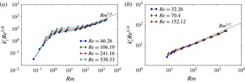
Figure 11.
 $k_{z}^{c}Re^{{\it\zeta}}$
as a function of
$k_{z}^{c}Re^{{\it\zeta}}$
as a function of
 $Rm$
for the different values of
$Rm$
for the different values of
 $Re$
shown in the legend, for the helical forcing case (a) and the non-helical forcing case (b).
$Re$
shown in the legend, for the helical forcing case (a) and the non-helical forcing case (b).

Figure 12. The critical magnetic Reynolds number
 $Rm_{c}$
as a function of the fluid Reynolds number
$Rm_{c}$
as a function of the fluid Reynolds number
 $Re$
. The two vertical dotted lines denote the two transition Reynolds numbers
$Re$
. The two vertical dotted lines denote the two transition Reynolds numbers
 $Re_{T_{1}},Re_{T_{2}}$
. The curves correspond to the non-helical forcing case.
$Re_{T_{1}},Re_{T_{2}}$
. The curves correspond to the non-helical forcing case.
6.2 Infinite layers
As seen in figure 4, in helical flows, due to the
 ${\it\alpha}$
effect for any
${\it\alpha}$
effect for any
 $Rm$
, there always exists
$Rm$
, there always exists
 $k_{z}$
small enough such that the modes are dynamo unstable. Thus, for a layer that is infinitely thick, a helical flow does not have a critical magnetic Reynolds number since unstable modes exist even for
$k_{z}$
small enough such that the modes are dynamo unstable. Thus, for a layer that is infinitely thick, a helical flow does not have a critical magnetic Reynolds number since unstable modes exist even for
 $Rm\rightarrow 0$
. However, for the non-helical case, there is a critical
$Rm\rightarrow 0$
. However, for the non-helical case, there is a critical
 $Rm$
for the dynamo instability as can be seen in figures 8 and 9. Below this
$Rm$
for the dynamo instability as can be seen in figures 8 and 9. Below this
 $Rm_{c}$
, for any mode
$Rm_{c}$
, for any mode
 $k_{z}$
, there is no dynamo instability. Thus, the critical magnetic Reynolds number
$k_{z}$
, there is no dynamo instability. Thus, the critical magnetic Reynolds number
 $Rm_{c}$
in the infinite domain is defined as
$Rm_{c}$
in the infinite domain is defined as
 $$\begin{eqnarray}\displaystyle Rm_{c}(Re)=\max \{Rm~\text{s.t.}~{\it\gamma}\leqslant 0~\forall k_{z}\}=\lim _{H\rightarrow \infty }Rm_{c}^{H}. & & \displaystyle\end{eqnarray}$$
Note that in practice we do not need an infinitely thick layer to capture the onset of the instability. However, the height
 $H$
needs to be sufficiently large to allow the first unstable mode
$H$
needs to be sufficiently large to allow the first unstable mode
 $k_{z}\simeq 1$
(as can be seen in figure 8) to be present. The dependence of
$k_{z}\simeq 1$
(as can be seen in figure 8) to be present. The dependence of
 $Rm_{c}$
as a function of
$Rm_{c}$
as a function of
 $Re$
can be seen in figure 12. Three different regimes corresponding to different flow behaviours are identified and these are separated by vertical dotted lines in the figure denoting the critical Reynolds numbers
$Re$
can be seen in figure 12. Three different regimes corresponding to different flow behaviours are identified and these are separated by vertical dotted lines in the figure denoting the critical Reynolds numbers
 $Re_{T_{1}}$
and
$Re_{T_{1}}$
and
 $Re_{T_{2}}$
. The curve for
$Re_{T_{2}}$
. The curve for
 $Re>Re_{T_{2}}$
corresponds to the turbulent regime at large
$Re>Re_{T_{2}}$
corresponds to the turbulent regime at large
 $Re$
and the curves in
$Re$
and the curves in
 $Re<Re_{T_{1}}$
,
$Re<Re_{T_{1}}$
,
 $Re_{T_{1}}<Re<Re_{T_{2}}$
correspond to two different laminar flows. Here,
$Re_{T_{1}}<Re<Re_{T_{2}}$
correspond to two different laminar flows. Here,
 $Re_{T_{2}}$
is the Reynolds number at which the flow transitions between a turbulent state and a laminar state, and
$Re_{T_{2}}$
is the Reynolds number at which the flow transitions between a turbulent state and a laminar state, and
 $Re_{T_{1}}$
is the Reynolds number at which the flow transitions between two different laminar time-independent flows. In the limit of large
$Re_{T_{1}}$
is the Reynolds number at which the flow transitions between two different laminar time-independent flows. In the limit of large
 $Re$
we see that the value of
$Re$
we see that the value of
 $Rm_{c}$
saturates as is observed in 3-D turbulent flows (Ponty et al.
Reference Ponty, Mininni, Montgomery, Pinton, Politano and Pouquet2005; Iskakov et al.
Reference Iskakov, Schekochihin, Cowley, McWilliams and Proctor2007; Mininni Reference Mininni2007) and the condensate case (Smith & Tobias Reference Smith and Tobias2004). Across the transition Reynolds numbers
$Rm_{c}$
saturates as is observed in 3-D turbulent flows (Ponty et al.
Reference Ponty, Mininni, Montgomery, Pinton, Politano and Pouquet2005; Iskakov et al.
Reference Iskakov, Schekochihin, Cowley, McWilliams and Proctor2007; Mininni Reference Mininni2007) and the condensate case (Smith & Tobias Reference Smith and Tobias2004). Across the transition Reynolds numbers
 $Re_{T_{2}}$
and
$Re_{T_{2}}$
and
 $Re_{T_{1}}$
, the
$Re_{T_{1}}$
, the
 $Rm_{c}$
curves have discontinuous behaviour because the flow transitions from one state to the other subcritically. In these laminar states, we find that the growth rate
$Rm_{c}$
curves have discontinuous behaviour because the flow transitions from one state to the other subcritically. In these laminar states, we find that the growth rate
 ${\it\gamma}$
scales as
${\it\gamma}$
scales as
 $k_{z}^{2}$
for very small
$k_{z}^{2}$
for very small
 $k_{z}$
as shown in figure 13 for
$k_{z}$
as shown in figure 13 for
 $Re=0.91<Re_{T_{1}}$
in the laminar regime. This scaling indicates that the dynamo action can be explained by the
$Re=0.91<Re_{T_{1}}$
in the laminar regime. This scaling indicates that the dynamo action can be explained by the
 ${\it\beta}$
effect, also known in the literature as the negative magnetic diffusivity effect (see Lanotte et al.
Reference Lanotte, Noullez, Vergassola and Wirth1999). The
${\it\beta}$
effect, also known in the literature as the negative magnetic diffusivity effect (see Lanotte et al.
Reference Lanotte, Noullez, Vergassola and Wirth1999). The
 ${\it\beta}$
effect is a mean field effect and the magnetic field is also amplified at the large scales. Figure 14 shows the contour of
${\it\beta}$
effect is a mean field effect and the magnetic field is also amplified at the large scales. Figure 14 shows the contour of
 $|B_{2\text{-}D}|^{2}=|b_{x}|^{2}+|b_{y}|^{2}$
, which is the energy of the magnetic field in the
$|B_{2\text{-}D}|^{2}=|b_{x}|^{2}+|b_{y}|^{2}$
, which is the energy of the magnetic field in the
 $x$
–
$x$
–
 $y$
plane. Two different Reynolds number are shown corresponding to the two different laminar states: on the left-hand side
$y$
plane. Two different Reynolds number are shown corresponding to the two different laminar states: on the left-hand side
 $Re_{T_{1}}<Re=5.4<Re_{T_{2}}$
and on the right-hand side
$Re_{T_{1}}<Re=5.4<Re_{T_{2}}$
and on the right-hand side
 $Re=0.53<Re_{T_{1}}$
. Both the plots show large-scale modulations in the magnetic energy at scales close to the box size.
$Re=0.53<Re_{T_{1}}$
. Both the plots show large-scale modulations in the magnetic energy at scales close to the box size.

Figure 13. The growth rate
 ${\it\gamma}$
as a function of
${\it\gamma}$
as a function of
 $k_{z}$
for a Reynolds number
$k_{z}$
for a Reynolds number
 $Re=0.91<Re_{T_{1}}$
together with a dotted line showing the scaling
$Re=0.91<Re_{T_{1}}$
together with a dotted line showing the scaling
 $k_{z}^{2}$
. The curve correspond to the non-helical forcing case.
$k_{z}^{2}$
. The curve correspond to the non-helical forcing case.

Figure 14. Contour of the magnetic energy
 $B_{2\text{-}D}$
for the two different laminar flows at two different
$B_{2\text{-}D}$
for the two different laminar flows at two different
 $Re$
– (a)
$Re$
– (a)
 $Re_{T_{1}}<Re\approx 5.4<Re_{T_{2}}$
, (b)
$Re_{T_{1}}<Re\approx 5.4<Re_{T_{2}}$
, (b)
 $Re\approx 0.53<Re_{T_{1}}$
. The contours correspond to the non-helical forcing case.
$Re\approx 0.53<Re_{T_{1}}$
. The contours correspond to the non-helical forcing case.
7 Dependence on
$k_{f}L$

In this section, we extend our study to flows with higher values of
 $k_{f}L$
. The linear damping coefficient is adjusted for each value of
$k_{f}L$
. The linear damping coefficient is adjusted for each value of
 $k_{f}L$
so that the maximum inertial range for the inverse cascade is obtained without forming condensates. As we increase
$k_{f}L$
so that the maximum inertial range for the inverse cascade is obtained without forming condensates. As we increase
 $k_{f}L$
, the inverse cascade becomes more important. Depending on the scale separation and the forcing used, the relative amplitude of
$k_{f}L$
, the inverse cascade becomes more important. Depending on the scale separation and the forcing used, the relative amplitude of
 $u_{2\text{-}D}$
and
$u_{2\text{-}D}$
and
 $u_{z}$
change as we change
$u_{z}$
change as we change
 $k_{f}L$
. Thus, in order to have a fair comparison between the different dynamos, we normalize the growth rates based on the results of the Ponomarenko dynamo (Ponomarenko Reference Ponomarenko1973) where the growth rate is proportional to the product of the vertical velocity
$k_{f}L$
. Thus, in order to have a fair comparison between the different dynamos, we normalize the growth rates based on the results of the Ponomarenko dynamo (Ponomarenko Reference Ponomarenko1973) where the growth rate is proportional to the product of the vertical velocity
 $\boldsymbol{u}_{z}$
and the planar velocity
$\boldsymbol{u}_{z}$
and the planar velocity
 $\boldsymbol{u}_{2\text{-}D}$
divided by the total root-mean-square value. Thus, we define a velocity scale
$\boldsymbol{u}_{2\text{-}D}$
divided by the total root-mean-square value. Thus, we define a velocity scale
 $U_{p}=(\langle |\boldsymbol{u}_{2\text{-}D}|^{2}\rangle ^{1/2}\langle u_{z}^{2}\rangle ^{1/2})/(\langle |\boldsymbol{u}_{2\text{-}D}|\rangle ^{2}+\langle |u_{z}|\rangle ^{2})^{1/2}$
with which we normalize the growth rate. Figure 15 shows the normalized growth rate
$U_{p}=(\langle |\boldsymbol{u}_{2\text{-}D}|^{2}\rangle ^{1/2}\langle u_{z}^{2}\rangle ^{1/2})/(\langle |\boldsymbol{u}_{2\text{-}D}|\rangle ^{2}+\langle |u_{z}|\rangle ^{2})^{1/2}$
with which we normalize the growth rate. Figure 15 shows the normalized growth rate
 ${\it\gamma}/(U_{p}k_{f})$
as a function of the normalized modes
${\it\gamma}/(U_{p}k_{f})$
as a function of the normalized modes
 $k_{z}/k_{f}$
for both helical and non-helical forcing as we increase
$k_{z}/k_{f}$
for both helical and non-helical forcing as we increase
 $k_{f}L$
for similar values of
$k_{f}L$
for similar values of
 $Re$
and
$Re$
and
 $Rm$
. Since
$Rm$
. Since
 $k_{f}$
is increased, the growth rate
$k_{f}$
is increased, the growth rate
 ${\it\gamma}$
and the number of unstable
${\it\gamma}$
and the number of unstable
 $k_{z}$
modes increase. The normalized curves seem to follow a similar trend for both the forcing cases considered here. At relatively large
$k_{z}$
modes increase. The normalized curves seem to follow a similar trend for both the forcing cases considered here. At relatively large
 $Rm$
and as the scale separation is increased, the most unstable wavenumber appears to be close to the forcing wavenumber
$Rm$
and as the scale separation is increased, the most unstable wavenumber appears to be close to the forcing wavenumber
 $k_{z}^{max}\approx k_{f}/3$
in both the helical and non-helical forcing cases. This implies that the most unstable modes have a similar length scale with forcing and not with the box size.
$k_{z}^{max}\approx k_{f}/3$
in both the helical and non-helical forcing cases. This implies that the most unstable modes have a similar length scale with forcing and not with the box size.

Figure 15.
 ${\it\gamma}/(U_{p}k_{f})$
as a function of
${\it\gamma}/(U_{p}k_{f})$
as a function of
 $k_{z}/k_{f}$
for different values of
$k_{z}/k_{f}$
for different values of
 $k_{f}$
for helical forcing on (a) and non-helical forcing on (b). The kinetic Reynolds number and the magnetic Reynolds number are mentioned in the legends.
$k_{f}$
for helical forcing on (a) and non-helical forcing on (b). The kinetic Reynolds number and the magnetic Reynolds number are mentioned in the legends.
The normalized maximum growth rate
 ${\it\gamma}_{max}/(U_{p}k_{f})$
and the normalized cutoff wavenumber
${\it\gamma}_{max}/(U_{p}k_{f})$
and the normalized cutoff wavenumber
 $k_{z}^{c}/k_{f}$
for both helical and non-helical forcing are shown in figure 16. As can be seen from the figures, the normalized quantities follow similar trends to
$k_{z}^{c}/k_{f}$
for both helical and non-helical forcing are shown in figure 16. As can be seen from the figures, the normalized quantities follow similar trends to
 $k_{f}L=4$
with weak (or no) dependence on the box size
$k_{f}L=4$
with weak (or no) dependence on the box size
 $L$
. Hence, the inverse cascade does not seem to affect the dynamo instability, and the mechanisms of the small-scale dynamo effect and the
$L$
. Hence, the inverse cascade does not seem to affect the dynamo instability, and the mechanisms of the small-scale dynamo effect and the
 ${\it\alpha}$
dynamo are mostly governed by the forcing scale where the strongest
${\it\alpha}$
dynamo are mostly governed by the forcing scale where the strongest
 $S_{2\text{-}D}$
shear exists.
$S_{2\text{-}D}$
shear exists.

Figure 16. Normalized growth rate:
 ${\it\gamma}_{max}/(U_{p}k_{f})$
on (a,c) and
${\it\gamma}_{max}/(U_{p}k_{f})$
on (a,c) and
 $k_{z}^{c}/k_{f}$
on (b,d) for (a,b) helical forcing and (c,d) non-helical forcing as a function of
$k_{z}^{c}/k_{f}$
on (b,d) for (a,b) helical forcing and (c,d) non-helical forcing as a function of
 $Rm$
for different
$Rm$
for different
 $k_{f}L$
as mentioned in the legends.
$k_{f}L$
as mentioned in the legends.
8 Conclusions
Our investigation examined the dynamo instability of 2.5-D flows for a wide range of control parameters. This allowed us to test certain limits that are still not attainable in 3-D simulations, and to test asymptotic theories and phenomenological expectations.
For helical flows, we were able to test the alpha dynamo predictions for the behaviour of the large scales (
 $k_{z}\ll k_{f}$
) both for small and large values of
$k_{z}\ll k_{f}$
) both for small and large values of
 $Rm$
and
$Rm$
and
 $Re$
. The analytical predictions of mean field theories for small values of
$Re$
. The analytical predictions of mean field theories for small values of
 $Rm$
were verified. For large values of
$Rm$
were verified. For large values of
 $Rm$
, the growth rates were also shown to be in agreement with a turbulent
$Rm$
, the growth rates were also shown to be in agreement with a turbulent
 ${\it\alpha}$
dynamo (calculated numerically from (4.2) and (4.3)), and the isotropic
${\it\alpha}$
dynamo (calculated numerically from (4.2) and (4.3)), and the isotropic
 ${\it\alpha}$
was shown to asymptote to a value independent of
${\it\alpha}$
was shown to asymptote to a value independent of
 $Re$
and
$Re$
and
 $Rm$
. At sufficiently large
$Rm$
. At sufficiently large
 $Rm$
, the fastest growing mode was always found to have
$Rm$
, the fastest growing mode was always found to have
 $k_{z}$
close to the forcing wavenumber. Thus, in a 3-D simulation with random initial conditions for the magnetic field, it is the scales close to the forcing scale that would be observed in the linear stage of the dynamo. This of course does not imply that the large-scale instability does not play a role in the saturated stage of the dynamo and the formation of large-scale magnetic fields at high
$k_{z}$
close to the forcing wavenumber. Thus, in a 3-D simulation with random initial conditions for the magnetic field, it is the scales close to the forcing scale that would be observed in the linear stage of the dynamo. This of course does not imply that the large-scale instability does not play a role in the saturated stage of the dynamo and the formation of large-scale magnetic fields at high
 $Rm$
. To resolve this issue, a nonlinear formalism for the
$Rm$
. To resolve this issue, a nonlinear formalism for the
 ${\it\alpha}$
dynamo would be required.
${\it\alpha}$
dynamo would be required.
The non-helical flows were also shown to result in dynamo instability above a value of the magnetic Reynolds number with similar behaviour to the helical dynamo at small scales
 $k_{z}\gtrsim k_{f}$
. The critical value of the magnetic Reynolds number for a thin layer of height
$k_{z}\gtrsim k_{f}$
. The critical value of the magnetic Reynolds number for a thin layer of height
 $H$
was shown to scale similarly to
$H$
was shown to scale similarly to
 $Rm_{c}^{H}\propto Re^{2{\it\zeta}}/\sqrt{H}$
with
$Rm_{c}^{H}\propto Re^{2{\it\zeta}}/\sqrt{H}$
with
 ${\it\zeta}\simeq 1/4$
for non-helical flows and
${\it\zeta}\simeq 1/4$
for non-helical flows and
 ${\it\zeta}\simeq 3/8$
for helical flows, implying that there is a dependence of
${\it\zeta}\simeq 3/8$
for helical flows, implying that there is a dependence of
 $Rm_{c}^{H}$
on
$Rm_{c}^{H}$
on
 $Re$
even at large values of
$Re$
even at large values of
 $Re$
. At infinite layer thickness
$Re$
. At infinite layer thickness
 $H$
, the helical flow always resulted in a dynamo (i.e.
$H$
, the helical flow always resulted in a dynamo (i.e.
 $Rm_{c}=0$
). On the other hand, the non-helical flow
$Rm_{c}=0$
). On the other hand, the non-helical flow
 $Rm_{c}$
asymptotically reached a finite value in the limit
$Rm_{c}$
asymptotically reached a finite value in the limit
 $Re\rightarrow \infty$
. It is worth pointing out that this asymptotic value
$Re\rightarrow \infty$
. It is worth pointing out that this asymptotic value
 $Rm_{c}\simeq 10$
is almost an order of magnitude smaller than what is obtained in 3-D simulations, and thus rotation could play a beneficial role in liquid-metal experiments.
$Rm_{c}\simeq 10$
is almost an order of magnitude smaller than what is obtained in 3-D simulations, and thus rotation could play a beneficial role in liquid-metal experiments.
The investigated dynamo flows were driven by rotating flows that tend to become 2-D at sufficiently large rotation rates. As discussed in the introduction, this is justified for layers of finite thickness and for the periodic boundary conditions above a critical rotation rate that have been considered here. In nature, rotating flows are never fully 2-D, either due to moderate rotation rates or boundary-layer effects.
For moderate rotation rates, large 2-D motions co-exist with 3-D perturbations in the form of travelling inertial waves. The resulting dynamo is then, in general, the result of a combination of these effects. However, due to the fast decorrelation time of inertial waves that has a dynamo suppressing effect (Herreman & Lesaffre Reference Herreman and Lesaffre2011), we expect that in rotating flows, even in the presence of some 3-D turbulent fluctuations, the 2.5-D part of the flow would be the dominant effect for a dynamo.
Boundary-layer effects are another way that a flow can deviate from 2-D behaviour in the fast rotating limit. For no-slip boundary conditions, the flow is known to vary rapidly along the rotation direction over a thin layer known as the Ekman layer (Ekman Reference Ekman1905; Pedlosky Reference Pedlosky1987). This layer is responsible for Ekman friction and the third component of velocity along the direction of rotation due to Ekman pumping. In this case, the amplitude of the third velocity component of the flow (that is essential for dynamo action) depends on the rotation rate. An asymptotic study that investigates these effects for a convection-driven dynamo in the presence of fast rotation was developed in Calkins et al. (Reference Calkins, Julien, Tobias and Aurnou2015, Reference Calkins, Julien, Tobias, Aurnou and Marti2016).
Further investigation of 3-D flows in the presence of rotation are required to address these issues.
Acknowledgements
The authors would like to thank F. Petrelis, S. Fauve and B. Gallet for their very useful comments and fruitful discussions. The present work benefited from the computational support of the HPC resources of GENCI-TGCC-CURIE and GENCI-CINES-JADE (project nos x2014056421 and x2015056421) and MesoPSL financed by the Region Ile de France and the project EquipMeso (reference ANR-10-EQPX-29-01) where the present numerical simulations have been performed.


