3.1. Visualizations

When the outer cylinder is stopped abruptly from a velocity greater than a given value, small vortices appear near the outer wall. Then, these vortices grow towards the IC and are rapidly destabilized. Finally, as no further energy is delivered to the flow, the vortex pattern decays. The whole process is presented for ${Re}_o =1700$ in a supplementary movie available at https://doi.org/10.1017/jfm.2021.346.

Figure 1 displays different time steps using binarized instantaneous images over the whole axial height ($z$) of the TC system at ${Re}_o=1700$. The instantaneous images were binarized, after being normalized by a mean image, using a Matlab function imbinarize with default value of 0.5 for the sensitivity parameter. The growth of the vortical structures can be observed from the moment they appear until they fill the whole gap width, which takes ${\approx }0.017$ viscous time units.

Figure 1. Binarized instantaneous images presenting the growth of vortical structures at different times steps for ${Re}_o=1700$ over the whole axial height ($z$) of the TC system. The $x$ and $y$ labels are the same for all panels as in (e): (a) $t = 0 tv/d^2$; (b) $t = 0.005 tv/d^2$; (c) $t = 0.01 tv/d^2$; (d) $t = 0.017 tv/d^2$; and (e) $t = 0.017 tv/d^2$ with zoom.

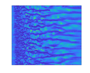
Taking the light intensity along a vertical line at mid-gap in each acquired image normalized with a mean image, we have constructed space–time diagrams. Figure 2 presents such space–time diagrams giving the variation in light intensity reflected by the Kalliroscope particles for three different outer Reynolds numbers ${Re}_o=870$, $1700$ and $17\,000$. They show the temporal evolution of the generation and decay of vortices and eventually turbulence. On the space–time diagrams, bright areas correspond to areas where Kalliroscope flakes move in the azimuthal direction whereas dark areas correspond to inwards or outwards motion in the radial direction.

Figure 2. Space–time diagram of the light intensity taken along $z$ near the outer cylinder for increasing outer Reynolds number with a stationary IC: (a) $Re_o = 8.7\times 10^2$; (b) $Re_o = 1.7\times 10^3$; (c) $Re_o = 1.7\times 10^3$ with zoom; and (d) $Re_o = 1.7\times 10^4$.

The minimum ${Re}_o$ at which vortex formation and decay are observed in the whole axial length is $870$. Vortices appear after the stoppage, merge and fade. However, for this ${Re}_o$ value, even if the merging of the vortices induces some defects and the flow is not turbulent (see figure 2a). On increasing ${Re}_o$, vortices still appear but rapidly undergo reorganization as they grow. We consider the formation of this disordered flow as the setting in of turbulence (see figure 2b–d). The higher the initial outer Reynolds number, the faster the stoppage generates turbulence throughout the axial length and the longer it lasts. It can also be seen in this figure that the size of the structures increases with time. They persist for a very long time and their persistence time increases with ${Re}_o$. At ${Re}_o=1.7\times 10^4$, they are still visible at $t\nu /d^2 = 0.4$.

We have estimated the size and growth of the vortices after they appear near the outer cylinder. This estimation was performed from the image obtained after binarization of the axially averaged images. We used the same binarization process as mentioned earlier. The initial vortex size $\langle \delta _i \rangle _z$ corresponds to the size the vortical structure when it first appears. This is presented in figure 3(a) as a function of the outer Reynolds number ${Re}_o$. It decreases with ${Re}_o$ and follows a power law which is well fitted by $a \times {Re}_o^{-2/3}$ as proposed by Kim & Choi (Reference Kim and Choi2004) for the critical wavelength of Taylor–Görtler vortices generated in an impulsively stopped rotating cylinder. Moreover, the best power law fit gives $n=-0.65$, which is very close to the expected $-2/3$ exponent.

Figure 3. Initial size of the vortices (a), their growth in linear (b) and in logarithmic scale (c) and the proportionality constant as a function of ${Re}_o$ (d). The legend in (a) is similar to that in (d), and the one in (b) represents (c) as well. In (c) the symbols represent experimental data and the black coloured lines represent fitted curves for the respective ${Re}_o$. The goodness of the fit varied between $0.97$ and $0.99$ for all power laws. In (d), all coefficients have $95\,\%$ confidence bounds, where the error bar represents the upper and lower bounds for each value of $a_{turb}$.

Figure 3(b) presents $\langle \delta _t \rangle _z$, the size of the vortical structures as a function of $\sqrt {t \nu /d^2}$ for different ${Re}_o$. This estimation was also obtained after binarization of the axially averaged images, but using an adaptive method with a sensitivity of $0.6$. In viscous time units, the time required by the vortices to fill up the gap width decreases with each increment in the ${Re}_o$. In a consistent way with respect to figure 3(a), the starting point for $\langle \delta _t \rangle _z$ decreases with increasing ${Re}_o$. Different growth phases can be distinguished for each ${Re}_o$. The initial growth phase is similar for all ${Re}_o>870$ with a mean growth rate of approximately $4.7$. The following growth phases also followed a power law, as such, it was pertinent to use a logarithmic scale to present it in figure 3(c). In this case, the ${Re}_o=870$ case was not plotted because it was not turbulent, as mentioned earlier. The curves intersect each other as $\langle \delta _t \rangle _z$ grows with $t \nu /d^2$ but differently for each ${Re}_o$. We found that they can all be well approximated by a power law fit with a same exponent of $1/2$ but each with a different proportionality constant $a_{turb}$, as can be observed in figure 3(c). Other exponents than $1/2$ do not give better results for the fit.

Our results are in very good agreement with the results of Kaiser et al. (Reference Kaiser, Frohnapfel, Ostilla-Monico, Kriegseis, Rival and Gatti2020) and Euteneuer & Karlsruhe (Reference Euteneuer and Karlsruhe1972) whose unstable zone grows as the square root of time. Following the idea that the vortices appear in the unstable zone as interpenetrating spirals do in the unstable zone between the inner cylinder and the nodal surface (the cylindrical surface where $u_{\theta }=0$) in counter-rotating TC flow, we can consider that $\langle \delta _t \rangle _z$ approximately corresponds to the size of the unstable zone of the flow. Kaiser et al. (Reference Kaiser, Frohnapfel, Ostilla-Monico, Kriegseis, Rival and Gatti2020) also observed multiple stages of $\sqrt {\nu t}$ growth, with each one separated by fast growth transition. In another similarity with the results of Kaiser et al. (Reference Kaiser, Frohnapfel, Ostilla-Monico, Kriegseis, Rival and Gatti2020) and Euteneuer & Karlsruhe (Reference Euteneuer and Karlsruhe1972), we have found that the coefficient $a_{turb}$ increases with ${Re}_o$, as presented in figure 3(d). We obtained a power law with an exponent of $1/2$ and a proportionality constant of $0.18$. Our power law exponent differs from the power law exponent of Kaiser et al. (Reference Kaiser, Frohnapfel, Ostilla-Monico, Kriegseis, Rival and Gatti2020), who obtained a value of $1/3$. However, Kaiser et al. (Reference Kaiser, Frohnapfel, Ostilla-Monico, Kriegseis, Rival and Gatti2020) presented the coefficient $a_{turb}$ as a ratio of $a_{turb}/a_{lam}$, where $a_{lam}$ is the proportionality factor for the growth of the laminar boundary layer thickness for their phase one and $a_{turb}$ corresponds to phase three.

3.2. Mean azimuthal velocity decay

Figure 4(a,b) presents the evolution of the mean azimuthal velocity with respect to time. The azimuthal velocity was averaged axially over 100 mm in the mid-height region, radially over 1.7 mm in the centre of gap region and at each instant of time with $t'=(i-5 f d/u_\theta ):(i+5 f d/u_\theta )$. To reduce the number of data points, every fifth data point is plotted in figure 4(a). The instantaneous visualization snapshots presented alongside the velocity decay demonstrate the evolution of the generation and decay processes. The visualization and PIV velocity estimations were conducted separately. Therefore, the insets in the figure 4(a) correspond to typical snapshots of the pattern as one may observe at that time steps. In figure 4(b), the time origin $t_0$ is fixed at time $t\nu /d^2= 0.034$ of figure 4(a)

Figure 4. Decay of azimuthal velocity with time at ${Re}_o=17300$. It is averaged axially, radially around the centre of gap-width over 2.7 mm and at each instant of time with $t'=(i-5 f d/u_\theta ):(i+5 f d/u_\theta )$. In (a) snapshots of instantaneous visualizations are also presented to show the evolution of the decay of the velocity for two different sets of data: repetitions 1 and 2. In (b) data set 1 was used to average with the different factors of 5 and 15. The time $t_0$ represents the time at which the stop occurs.

In figure 4(a) it seems that the mean azimuthal velocity's rate of decay follows a power law of the type $y=ax^n$. However, when only the decay region is observed in figure 4(b), it can be seen that this decay does not follow a single power law, as also observed by Ostilla-Mónico et al. (Reference Ostilla-Mónico, Zhu, Spandan, Verzicco and Lohse2017). Multiple decay regions can be observed in figure 4(b). We have identified three phases for the whole turbulence generation and decay process. These three phases can be better understood with the observation of the variation of the turbulent kinetic energy in the following sub-section.

An important aspect to be observed is the free decay of the azimuthal velocity profile as a function of time (figure 5). Figure 5(a) gives the azimuthal velocity profile at different time steps of the decay period, as shown in figure 4(b). The azimuthal velocity is averaged axially and at each instant of time using the moving average method mentioned earlier. A selected few time steps were chosen to present the decay of the turbulence. As for the visualizations, ${Re}_o=1700$ is chosen to present the decay process of the mean azimuthal radial profile over the first 0.05 viscous time units. At ${Re}_o=17\,300$, this decay process was much faster and took just 0.01 viscous time units for the radial profile to reach below 40 % of the maximum azimuthal velocity component. The two first profiles, for $t=0$ and $0.0001 (t-t_0) \nu /d^2$, are very close to the analytical Couette profile, which is represented by the analytical profile presented as the dotted line. Then, as the outer cylinder is stopped, the following profiles remain close to the Couette flow in the first half of the gap, reach a maximum value, termed $u_{\theta max}$, and decrease towards zero. Our measurements did not allow us to observe the decrease toward zero near the outer cylinder. These profiles are similar to the ones observed in spin-down experiments (Kim et al. Reference Kim, Song and Choi2008; Kaiser et al. Reference Kaiser, Frohnapfel, Ostilla-Monico, Kriegseis, Rival and Gatti2020). The shape and structure of the azimuthal velocity profiles demonstrate that the unstable region lies near the outer cylinder for the current configuration, which can also be confirmed in figure 1.

Figure 5. Radial decay process observed experimentally at ${Re}_o=1700$ (a) and its theoretical explanation (b). In (a) mean azimuthal velocity is averaged axially and at each instant of time with $t'=(i-5 f d/u_\theta ):(i+5f d/u_\theta )$. The dotted line represents the analytic laminar profile. The time $t_0$ represents the time at which the stop occurs.

Figure 5 was constructed after estimating the actual point of stoppage, which could be observed clearly for the visualization experiments, but is not known as well for the stereo-PIV measurements. Based on figure 4, we can deduce the actual time frame at which the decay starts; however, the question remains as to whether the point at which decay starts is the same as that at which the stop occurs. However, this decay process allows us to ascertain that, at the instance of stoppage, the azimuthal velocity component at the outer cylinder wall will fall towards zero and cause the decay observed in figure 5. As a result, it is fair to assume that the point of decay is the point of stoppage as well.

As demonstrated in figure 5(b), as soon as the cylinder is stopped, the velocity of the outer cylinder wall becomes zero. The wall velocity at the IC is already zero (because the inner cylinder is stationary), but the velocity in the gap width remains non-zero. This creates a centrifugally unstable region viz-a-viz Rayleigh's criterion (Rayleigh Reference Rayleigh1917), which states that if the Rayleigh discriminant is positive an instability may develop. Hence, as soon as the outer cylinder wall velocity becomes zero, Rayleigh's discriminant becomes positive in the region between the position of $u_{\theta max}$ and the outer cylinder, creating the possibility of a centrifugal instability. At the first stage of the instability, the unstable region and the resulting vortices are located in the immediate vicinity of the outer cylinder. As stated by Neitzel (Reference Neitzel1982) for experiments of Couette flow decay, the IC has probably no influence on the instability at this stage. These vortical structures grow along with the thickness of the unstable region. Therefore, the pattern requires continuous reorganization that leads to its irregularity and the development of turbulence in the system, depending upon the Reynolds number (figure 2). These structures propagate towards the inner cylinder (figure 1), with the growth rate depending on the Reynolds number, as explained earlier. Similar observations were reported by Euteneuer & Karlsruhe (Reference Euteneuer and Karlsruhe1972) and Neitzel & Davis (Reference Neitzel and Davis1981).

Figure 6 presents the azimuthal velocity profile corresponding to the instance at which decay starts at different ${Re}_o$. It was averaged in a similar way as the case for figure 5. It demonstrates the size of the unstable zone which could be governing the appearance of the vortices. It is known that the size of the zone between the nodal surface and IC walls plays a critical role in the localization and size of the vortices induced by the destabilization of the counter-rotating Couette flow (Esser & Grossmann Reference Esser and Grossmann1996). Similarly, the zone between the inflection point, observable in figure 6, and the outer cylinder wall must determine the appearance and the size of the vortical structures.

Figure 6. Azimuthal velocity at the instance at which decay starts for different ${Re}_o$. It is averaged axially and at each instant of time with $t'=(i-5 f d/u_\theta ):(i+5 f d/u_\theta )$. The vertical red line points towards the inflection point observable at the presented Reynolds number.

3.3. Kinetic energy decay

Figures 7 and 8 demonstrate the decay of the three forms of the kinetic energy (KE): mean, turbulent and wind. The presented data are averaged axially, radially near the centre of the gap for figure 7 and near the inner and outer cylinders for figure 8, and at each instant of time with $t'=(i-5 f d/u_\theta ):(i+5 f d/u_\theta )$. Figure 7(a–c) presents a comparison for the three types of KE at different ${Re}_o$, while figures 7(d) and 8 depict these three types of KE only for ${Re}_o=1.7\times 10^4$. All the temporal scales in figures 7 and 8 are made dimensionless using the dynamic time scale $r_o \omega /d$ to facilitate comparison between different ${Re}_o$. Additionally, all the temporal profiles for these kinetic energies start from the moment stop occurs, as discussed for figure 4. The mean KE was estimated from the mean velocity flow components: $k_{mean}=1/2(\langle u_r\rangle _{t',z}^{2}+\langle u_\theta \rangle _{t',z}^{2}+\langle u_z\rangle _{t',z}^{2})$, where $r$ and $z$ represent the radial and axial coordinates. The turbulent KE is estimated from the fluctuating radial, azimuthal and axial components of the velocity as: $k_{turb}=1/2((\langle u_r'^{2}\rangle _{t',z}+(\langle u_\theta '^{2}\rangle _{t',z}+(\langle u_z'^{2}\rangle _{t',z})$, where $u_{r,\theta , z}'=u_{r,\theta ,z}-\langle u_{r,\theta ,z}\rangle _{t',z}$. And finally, the wind KE was composed of only the radial and axial fluctuating components of the velocity: $k_{wind}=1/2(\langle u_r'^{2}\rangle _{t',z}+\langle u_z'^{2}\rangle _{t',z})$. It can be noticed that the general behaviour of the three kinetic energies is the same for all ${Re}_o$. As the Reynolds number fixed the initial conditions of the decay process, this means that this initial condition has no impact on the general behaviour of the decay. Temporal re-scaling with the $r_o \omega /d$ term makes the decay profile longer for increasing ${Re}_o$. Considering the similar behaviour for all ${Re}_o$, we compare directly the three kinetic energies in figure 7(d) for the largest ${Re}_o$.

Figure 7. Temporal evolution of the dimensionless mean (a), turbulent (b) and wind KE (c) at different Reynolds numbers, and these three together for ${Re}_o=1.7\times 10^4$ (d). These are averaged axially, radially around the centre of the gap over 1.7 mm and at each instant of time with $t'=(i-5 f d/u_\theta ):(i+5 f d/u_\theta )$. The $x$ and $y$ labels for (a,b) are same as those in (c,d). Also, the legend in (b,c) is same as that in (a). The time $t_0$ represents the time at which the stop occurs.

Figure 8. Temporal evolution of the dimensionless mean, turbulent and wind KE at ${Re}_o=17\,300$ when radially averaged near the inner (black markers) and outer (red markers) cylinders. These are averaged axially, radially around the IC (black markers) and outer cylinder (red markers) over 1.7 mm and at each instant of time with $t'=(i-5 f d/u_\theta ):(i+5 f d/u_\theta )$. The time $t_0$ represents the time at which the stop occurs.

The mean KE follows the mean azimuthal velocity profile and decays continuously with time. The turbulent and wind KE profiles show different phases for this turbulence generation and decay process. When the outer cylinder is rotating, its vibration generates experimental noise which gives the initial value for the turbulence and wind kinetic energies. As the outer cylinder is stopped, the turbulence sets in and these kinetic energies start to grow until they reach their maximum value. This generation of turbulence is considered as phase I of this generation and decay process. As also observed in figure 2, this initial phase is marked by the generation of small vortical structures, resulting in the centrifugal instability. These small scale structures induce radial and axial components of the velocity, resulting in an increase in the wind KE, as observed in figure 7(d). At the centre of the gap, the time at which the maximum is reached is $49 t r_o \omega /d$; whereas it is $100$ near the IC, as can be seen in figure 8. Near the outer cylinder, there is a small initial decrease followed by a small plateau at $t r_o \omega /d$ between 31 and 45. At this location, the mean, turbulent, and wind KE are close to their maximal value. When the cylinder is stopped, the fluctuations slightly decrease with the velocity but the emergence of the structures maintain its high level. Then, as the velocity further decreases, the decay process starts and the wind and turbulence kinetic energies decrease from their maximum values at the centre and near the IC and from the plateau near the outer cylinder. This occurs at different times for each position along the gap. This time difference between the different starting points of the decay comes from the propagation of the structures from the outer cylinder towards the IC as they grow (figure 1). Kaiser et al. (Reference Kaiser, Frohnapfel, Ostilla-Monico, Kriegseis, Rival and Gatti2020) observed a similar phenomenon in their Phase-II, which they termed as the ‘emergence of Taylor rolls and laminar-to-turbulent transition’. Evidently, this initial phase is not present if the flow is already turbulent before the stop occurs, as in the results of Verschoof et al. (Reference Verschoof, Huisman, van der Veen, Sun and Lohse2016) and Ostilla-Mónico et al. (Reference Ostilla-Mónico, Zhu, Spandan, Verzicco and Lohse2017). There is no generation of turbulence occurring in this case, which could have led to an increase in the turbulent KE.

Once the maximum is reached, the decay of the turbulent and wind KE starts. This decay phase is named phase II in figure 7(d). We found that the wind KE appears to follow a power law with the power exponent of $-$1.36. This falls between the HIT based theoretical predictions of $-6/5$, and $-10/7$ for the Saffman (Reference Saffman1967) and Kolmogorov (Reference Kolmogorov1941) theories, respectively. Phase II is defined by the merger of smaller scale structures towards larger scales together with their fading. This process is repeated until the final phase (phase III in figure 7d), which is dominated by viscous diffusion (figure 2). The merging of structures leads to the reorganization of the energy and the length scales continuously. During this process of reorganization, multiple plateaus can be remarked upon, for example the biggest one around $150~t r_o \omega /d$ of decay in figure 7(d). These plateaus are visible around the centre and near the IC but not near the outer cylinder (figures 7(d) and 8). The fusion of the structures at certain instances sustains the KE causing these plateaus, this process can also be observed in Ostilla-Mónico et al. (Reference Ostilla-Mónico, Zhu, Spandan, Verzicco and Lohse2017). Once this fusion stops, the decay process enters the final phase during which the large scale structures decay under the influence of viscous diffusion.

Towards the end of this final decay phase, the turbulent KE is higher in magnitude compared with the mean KE; even though at this stage the flow cannot be considered as turbulent. This occurred whatever the measurement position was. At this stage, we observe large vortical structures having an axial periodicity and propagating tangentially as axisymmetric rolls which decay with time, as can be observed in figure 2. Following the idea of Hussain & Reynolds (Reference Hussain and Reynolds1970), these vortical structures with their axial periodicity can be associated with a wave component in the velocity decomposition process. In this process, $u=\langle u\rangle +u'$, where $u'=u_{wave}+u_{turbulence}$. In our case, there is a non-separation of the wave component from the fluctuating velocity component (Hussain & Reynolds Reference Hussain and Reynolds1970) which forms the turbulent KE. As such, the turbulent KE represents both the wave component due to the vortical structures and the fluctuating component. At the end of the decay process, $u'$ is mainly composed of the wave component.

3.4. Energy dissipation rate and length scales

Figure 9(a) presents the production of KE and the mean, turbulent and total KE dissipation rates estimated using 7 out of the 12 gradients using the cylindrical coordinates (Pope Reference Pope2000). The direct estimation of the energy dissipation of the mean KE, turbulent KE and total KE can be estimated from equations (3.1), (3.2) and (3.3), respectively. The current PIV measurements were stereo-PIV, which provides access to the three velocity components but only two set of coordinates. As such, out of the total 12 components for the direct estimation of the dissipation of the mean, turbulent and total KE, only seven were estimated here because the other five components required the azimuthal coordinate which was not accessible, as shown in (3.4), (3.5) and (3.6). Nonetheless, Singh (Reference Singh2016) have shown that the missing five components related to the azimuthal coordinate make a negligible contribution to the estimation of the mean KE dissipation rate with more than 90 % contribution coming from the gradients of the radial coordinate. The symmetry of the roll structures that appear in this case is similar to that of turbulent Taylor vortex flow. Moreover, these missing five components can be estimated using Taylor's hypothesis, which would give $\partial \theta =u_\theta \partial t/r.$ A brief analysis of these components showed a less than $0.01\,\%$ contribution towards the mean energy dissipation rate estimation. Consequently, the prediction based on the seven components was maintained. These gradients were estimated using the second-order central differencing approximation of the first derivative (Singh Reference Singh2016).

Figure 9. Temporal evolution of the production and dissipation of energy and two length scales at ${Re}_o=17\,300$. The inset in b presents the multiple power laws observed in the Taylor microscale. These are averaged axially, radially around the centre of the gap width over 1.7 mm and at each instant of time with $t'=(i-5 f d/u_\theta ):(i+5 f d/u_\theta )$. The time $t_0$ represents the time at which the stop occurs.

Based on the estimation of the dissipation rate, the Taylor microscale, $\langle \lambda \rangle =\sqrt {15\nu \langle u_\theta ^{'2}\rangle /\langle \epsilon _{mean} \rangle }$, and Kolmogorov scale, $\langle \eta _K\rangle =(\nu ^3/\langle \epsilon _{mean} \rangle )^{(1/4)}$ were also estimated. These two length scales are presented in figure 9(b). On the other hand, the production of KE was estimated as: $P=-\langle u_\theta ' u_r'\rangle (\textrm {d} \langle u_\theta \rangle /\textrm {d} r-u_\theta /r)$. Figure 9(a,b) shows only the data corresponding to phases I and II of the KE, except for the profile of the total energy dissipation. Only phases I and II were chosen because the viscous decay phase III was practically diffusive in nature and contained insignificant fluctuating content, as can be observed with the temporal evolution of the turbulent and wind KE (figure 7)

(3.1)\begin{align} \epsilon_{mean_{all}} &=\nu \left \lbrace 2 \left( \left( \frac{\partial \overline{U_r}}{\partial r}\right)^ 2+ \left( \frac{1}{r} \frac{\partial \overline{U_\theta}}{\partial \theta}+\frac{\overline{U_r}}{r} \right)^2+\left( \frac{\partial \overline{U_z}}{\partial z} \right)^2 \right)+\left( r \frac{\partial \overline{(U_\theta/r)}}{\partial r}\right)^2 \right. \nonumber\\ &\quad \left. +\left(\frac{1}{r}\frac{\partial\overline{U_r}}{\partial \theta}\right)^2+\left(\frac{1}{r}\frac{\partial\overline{U_z}}{\partial \theta}\right)^2 +\left(\frac{\partial\overline{U_z}}{\partial r}\right)^2+\left(\frac{\partial\overline{U_r}}{\partial z}\right)^2+\left(\frac{\partial \overline{U_\theta}}{\partial z}\right)^2 \right. \nonumber\\ &\quad \left.\vphantom{\left( \frac{\partial \overline{U_r}}{\partial r}\right)^ 2} +2\left(\frac{\partial \overline{(U_\theta/r)}}{\partial r}\cdot \frac{\partial \overline{U_r}}{\partial \theta}+\frac{1}{r}\frac{\partial \overline{U_\theta}}{\partial z}\cdot \frac{\partial \overline{U_z}}{\partial \theta}+\frac{\partial \overline{U_r}}{\partial z}\cdot \frac{\partial \overline{U_z}}{\partial r}\right) \right\rbrace , \end{align}

(3.2)\begin{align} \epsilon_{turb_{all}} &=\nu \left \lbrace 2 \left( {\left( \frac{\partial {u_r^{'}}}{\partial r}\right)^ 2}+ {\left( \frac{1}{r} \frac{\partial {u_\theta^{'}}}{\partial \theta} +\frac{{u_r^{'}}}{r}\right)^2}+{\left( \frac{\partial {u_z^{'}}}{\partial z} \right)^2} \right)+{ \left(r\frac{\partial{(u_\theta^{'}/r)}}{\partial r}\right)^2} \right. \nonumber\\ &\quad \left. +{\left(\frac{1}{r}\frac{\partial {u_r^{'}}}{\partial \theta}\right)^2}+{\left(\frac{1}{r}\frac{\partial{u_z^{'}}}{\partial \theta}\right)^2} +{\left(\frac{\partial{u_z^{'}}}{\partial r}\right)^2}+{\left(\frac{\partial {u_r^{'}}}{\partial z}\right)^2} + {\left(\frac{\partial {u_\theta^{'}}}{\partial z}\right)^2} \right. \nonumber\\ &\quad \left.\vphantom{ \left(r\frac{\partial{(u_\theta^{'}/r)}}{\partial r}\right)^2} +2\left({\frac{\partial {(u_\theta^{'}/r)}}{\partial r}\cdot \frac{\partial {u_r^{'}}}{\partial \theta}}+ {\frac{1}{r} \frac{\partial {u_\theta^{'}}}{\partial z}\cdot \frac{\partial {u_z^{'}}}{\partial \theta}}+{\frac{\partial {u_r^{'}}}{\partial z}\cdot \frac{\partial {u_z^{'}}}{\partial r}}\right) \right\rbrace , \end{align}

(3.3)\begin{align} \epsilon_{total_{all}} &=\nu \left \lbrace 2 \left( \left( \frac{\partial {U_r}}{\partial r}\right)^ 2+ \left( \frac{1}{r} \frac{\partial {U_\theta}}{\partial \theta}+\frac{{U_r}}{r} \right)^2+\left( \frac{\partial{U_z}}{\partial z} \right)^2 \right)+\left( r \frac{\partial {(U_\theta/r)}}{\partial r}\right)^2 \right. \nonumber\\ &\quad \left. +\left(\frac{1}{r}\frac{\partial{U_r}}{\partial \theta}\right)^2+\left(\frac{1}{r}\frac{\partial{U_z}}{\partial \theta}\right)^2 +\left(\frac{\partial{U_z}}{\partial r}\right)^2+\left(\frac{\partial{U_r}}{\partial z}\right)^2+\left(\frac{\partial {U_\theta}}{\partial z}\right)^2 \right. \nonumber\\ &\quad \left.\vphantom{\left( r \frac{\partial {(U_\theta/r)}}{\partial r}\right)^2} +2\left(\frac{\partial {(U_\theta/r)}}{\partial r}\cdot \frac{\partial {U_r}}{\partial \theta}+\frac{1}{r}\frac{\partial{U_\theta}}{\partial z}\cdot \frac{\partial {U_z}}{\partial \theta}+\frac{\partial{U_r}}{\partial z}\cdot \frac{\partial {U_z}}{\partial r}\right) \right\rbrace , \end{align}

(3.4)\begin{align} \epsilon_{mean} &=\nu \left( 2 \left( \left( \frac{\partial \overline{U_r}}{\partial r}\right)^ 2+\left( \frac{\partial \overline{U_z}}{\partial z} \right)^2 \right)+ \left( r \frac{\partial \overline{(U_\theta/r)}}{\partial r}\right)^2 +\left(\frac{\partial\overline{U_z}}{\partial r}\right)^2+ \left(\frac{\partial\overline{U_r}}{\partial z}\right)^2\right. \nonumber\\ &\quad \left. +\left(\frac{\partial\overline{U_\theta}}{\partial z}\right)^2 +2 \frac{\partial \overline{U_r}}{\partial z}\cdot \frac{\partial \overline{U_z}}{\partial r} \right), \end{align}

(3.5)\begin{align} \epsilon_{turb} &=\nu \left( 2 \left( {\left( \frac{\partial {u_r^{'}}}{\partial r}\right)^ 2}+{\left( \frac{\partial {u_z^{'}}}{\partial z} \right)^2} \right)+ {\left(r\frac{\partial{(u_\theta^{'}/r)}}{\partial r}\right)^2}+{\left(\frac{\partial {u_z^{'}}}{\partial r}\right)^2}+{\left(\frac{\partial {u_r^{'}}}{\partial z}\right)^2}\right. \nonumber\\ &\quad \left. +{\left(\frac{\partial {u_\theta^{'}}}{\partial z}\right)^2}+2{\frac{\partial {u_r^{'}}}{\partial z}\cdot \frac{\partial {u_z^{'}}}{\partial r}} \right) , \end{align}

(3.6)\begin{align} \epsilon_{total} &= \nu \left( 2 \left( \left( \frac{\partial {U_r}}{\partial r}\right)^ 2+\left( \frac{\partial{U_z}}{\partial z} \right)^2 \right)+ \left( r \frac{\partial {(U_\theta/r)}}{\partial r}\right)^2 +\left(\frac{\partial{U_z}}{\partial r}\right)^2+\left(\frac{\partial{U_r}}{\partial z}\right)^2\right. \nonumber\\ &\quad \left. +\left(\frac{\partial {U_\theta}}{\partial z}\right)^2 +2\frac{\partial {U_r}}{\partial z}\cdot \frac{\partial {U_z}}{\partial r} \right). \end{align}

The turbulent KE dissipation rate and the production of KE increased in phase I (figure 9a). This further confirms that phase I is defined by the generation of KE. The initial (first three points) higher magnitude of the production of KE and the turbulent KE dissipation rate is due to the vibration of the outer cylinder while it was rotating before the stop, as mentioned earlier. Phase II starts with the decay of all energy dissipation rates. During this decay process large oscillations of the production of KE occur together with small oscillations of all the KE dissipation rates. During this phase the reorganization of the vortices also occurs. This induces the oscillations of the turbulent and mean KE dissipation rates but at different instances. The behaviour of the total KE dissipation rate, which is the sum of the turbulent and mean KE dissipation rates, reflects its two component oscillations. The production of KE represents the transfer of energy between the turbulent and mean components of the flow. Its oscillations correspond to the oscillations of the total KE dissipation rate. Towards the end of phase II, the turbulent KE dissipation rate was higher in magnitude than the mean KE dissipation rate. As explained earlier, the turbulent component, presented herein, consists of both the fluctuating and periodic components. Towards the end of the decay phase, the fluctuating component is negligible, so that the turbulent KE mainly consists of the periodic component which is due to axisymmetric vortices. This will continue until these vortices vanish completely. This is the main reason for a higher turbulent KE dissipation rate than the mean KE dissipation rate towards the end of decay process. As a consequence, the profile of the total KE dissipation rate is similar to that of the turbulent KE dissipation rate. Verschoof et al. (Reference Verschoof, Huisman, van der Veen, Sun and Lohse2016) and Ostilla-Mónico et al. (Reference Ostilla-Mónico, Zhu, Spandan, Verzicco and Lohse2017) presented a total KE dissipation rate that is more similar to the profile of the mean KE dissipation rate presented here. In the case of Verschoof et al. (Reference Verschoof, Huisman, van der Veen, Sun and Lohse2016) and Ostilla-Mónico et al. (Reference Ostilla-Mónico, Zhu, Spandan, Verzicco and Lohse2017), there was no generation of turbulence, and decay only happened from the moment the IC was brought to a stop. George (Reference George1992) stated that the Taylor microscale should be considered as the characteristic length scale, and that it increases as the square root of time, or $\lambda \sim t^{1/2}$. An increase, following a power law, could be seen at multiple times but not constantly in phases I and II, see figure 9(b). The power law exponent increases from $0.1$ to $1$ as a function of time, as can be observed from the inset in figure 9(b). Moreover, the Taylor microscale, which is known to play a dominant role in the energy and momentum transfer, captures well the reorganization of energy. The Kolmogorov scale is constant during the first 100 inertial time units and it then increases monotonically with time. This scale, by definition, is inversely proportional to the mean KE dissipation rate, which is clearly visible in its temporal profile. The reorganization of the length scales and the energy are not as visible in the mean KE dissipation rate, and consequently not represented by the Kolmogorov scale. As such, the Taylor microscale better describes the decay of energy, and should be considered as the length scale for phases I and II instead of the Kolmogorov scale, even though the increase as the square root of time was not observed.

3.5. Self-similarity

Figure 10 presents the self-similarity picture for the radial profile azimuthal velocity at ${Re}_o=17\,300$ for the decay phases. The velocity profile was averaged axially and over time, and normalized with its spatial average. This was formed based on the self-similarity criterion presented by Verschoof et al. (Reference Verschoof, Huisman, van der Veen, Sun and Lohse2016). They defined the criterion for self-similarity as that, when the azimuthal velocity profiles averaged over $\theta$ are normalized with the spatial mean of the azimuthal velocity averaged radially and azimuthally, the profiles overlapped each other. The only difference with their method being that, instead of using azimuthal velocity profiles averaged over $\theta$, the azimuthal velocity was averaged axially and over time. A complete self-similarity covering the whole decay process was not seen. Instead, profiles under phase II were found to be self-similar among themselves but not much in the final phase. Verschoof et al. (Reference Verschoof, Huisman, van der Veen, Sun and Lohse2016) observed self-similarity only in the intermediate region, whereas Ostilla-Mónico et al. (Reference Ostilla-Mónico, Zhu, Spandan, Verzicco and Lohse2017) observed self-similarity in the final decay phase.

Figure 10. Radial profile of azimuthal velocity averaged axially and over time, for $t'=(i-5f d/u_\theta ):(i+5f d/u_\theta )$, and normalized with its spatial mean value at ${Re}_o=17\,300$. The time represents the instant at which the profile was extracted from the moment decay started.

Earlier, George (Reference George1992) stated different characteristics for a self-preserving solution: $\lambda$ and $R_\lambda =u' \lambda /\nu$ as the characteristic length scale and turbulence Reynolds number respectively; energy decay follows a power law; the Taylor microscale can be predicted as the square root of time; constants of proportionality and the exponent vary with respect to the initial condition; and finally the spectrum and spectral functions collapse when plotted. As per the characteristics of a self-preserving solution defined by George (Reference George1992), some similarities could be seen. Most notably, the Taylor microscale, $\lambda$, could be considered as the characteristic length scale based on its temporal evolution depiction in figure 9(b). Energy decay was observed to be following a power law, but not a single power law that could define the whole decay process due to the reorganization of structures and length scales, as can be observed in figures 7 and 8.

On the other hand, it is crucial to observe how the decay will occur at a much larger outer cylinder Reynolds number, of the order of $10^6$. If this can be done experimentally it would be much better. This was not feasible in the current geometry due to technical constraints. Otherwise, a numerical approach can definitely shed some light on this subject, as demonstrated by Ostilla-Mónico et al. (Reference Ostilla-Mónico, Zhu, Spandan, Verzicco and Lohse2017) and Kaiser et al. (Reference Kaiser, Frohnapfel, Ostilla-Monico, Kriegseis, Rival and Gatti2020). The numerical studies can provide results in the whole domain, especially in the boundary layer region and with respect to wall friction, and geometrical configurations can be modified much more easily.