


1 Introduction
Small, heavy particles in an inhomogeneous turbulent flow tend to migrate from regions of high turbulence intensity toward lower-intensity regions (Caporaloni et al. Reference Caporaloni, Tampieri, Trombetti and Vittori1975; Reeks Reference Reeks1983). This phenomenon, known as turbophoresis, is driven by a differential in turbulent dispersion rates between different regions of a flow. Particles in regions with higher turbulent intensity disperse more quickly than those in more quiescent regions, causing particles to accumulate with longer residence times and higher concentrations in regions of lower turbulence intensity. In wall-bounded turbulent flows, no-slip and no-penetration conditions cause turbulence intensities to vanish at solid boundaries, resulting in sharp gradients of turbulence intensity in the viscous sublayer and buffer region. As a result, particles tend to accumulate in the viscous sublayer (Marchioli & Soldati Reference Marchioli and Soldati2002; Sikovsky Reference Sikovsky2014) at high concentrations relative to the surrounding flow. The increased concentration near the wall can influence a number of physical processes, such as deposition (Guha Reference Guha2008), collision and coalescence (Kuerten & Vreman Reference Kuerten and Vreman2015; Kuerten Reference Kuerten2016) and radiation transmission and absorption (Pouransari & Mani Reference Pouransari and Mani2017).
Using direct numerical simulations (DNS) to predict turbulent wall-bounded flows is currently feasible only up to moderate Reynolds numbers, because the computational cost increases very quickly with Reynolds number (Moin & Mahesh Reference Moin and Mahesh1998). Because DNS is prohibitively expensive for high Reynolds number engineering flows, large-eddy simulations (LES) have enjoyed a good deal of success and popularity in recent decades. Because LES can only represent a coarse-grained version of the turbulent carrier flow, the effect of small-scale turbulence on particles requires additional modelling. Armenio, Piomelli & Fiorotto (Reference Armenio, Piomelli and Fiorotto1999) showed the effect of using LES instead of DNS to advance tracer and inertial particle trajectories, finding that tracer particles are actually the most sensitive to small-scale motions in terms of single-particle statistics. Marchioli, Salvetti & Soldati (Reference Marchioli, Salvetti and Soldati2008b) also pointed out the insufficiency of LES alone for advancing particle trajectories, showing the impact of subgrid scales on particle concentration profiles and clustering in a turbulent channel flow. Further, Marchioli, Salvetti & Soldati (Reference Marchioli, Salvetti and Soldati2008a) showed that simply recovering the subgrid-scale fluctuation energy through approximate deconvolution or fractal interpolation may not be enough for accurate prediction of these phenomena. Bianco et al. (Reference Bianco, Chibbaro, Marchioli, Salvetti and Soldati2012) further studied the statistics of errors due to using a filtered velocity field to advance particles, emphasizing the effect of particles sampling in a biased way the near-wall flow features such as streaks, sweeps, and ejections.
The LES approach is based on resolving the dominant, most energetic motions in a flow while leaving smaller, less influential fluctuations unresolved (and represented by a subgrid stress model). In wall-bounded turbulent flows, the size of energetic motions decreases close to the wall, so that computational grids must be refined in all directions to resolve the most influential flow features in the near-wall region and apply the no-slip, no-penetration boundary conditions – a practice referred to as wall-resolved LES (WRLES). As a result, WRLES does contain at least some information, albeit incomplete, about near-wall turbulent fluctuations. Significant attention has been paid in recent years to enriching WRLES for particle-laden flows with models for subgrid-scale (SGS) fluctuations, as recently reviewed by Kuerten (Reference Kuerten2016) and Marchioli (Reference Marchioli2017). The main closure problem in this context is that, to solve for particle dynamics using a drag law, the fluid velocity seen by the particle, including subgrid motions, is needed. For modelling the subgrid fluid velocity seen by particles, various approaches include: approximate deconvolution (Kuerten Reference Kuerten2006; Park et al. Reference Park, Bassenne, Urzay and Moin2017), kinematic simulation (Ray & Collins Reference Ray and Collins2014), fractal interpolation (Scotti & Meneveau Reference Scotti and Meneveau1999) and stochastic methods (Fede et al. Reference Fede, Simonin, Villedieu and Squires2006; Pozorski & Apte Reference Pozorski and Apte2009; Minier Reference Minier2015; Innocenti, Marchioli & Chibbaro Reference Innocenti, Marchioli and Chibbaro2016; Breuer & Hoppe Reference Breuer and Hoppe2017). Some of these models are developed in the context of homogeneous turbulence while others are valid for inhomogeneous or near-wall flows. Stochastic models for subgrid scales in LES have been informed by similar techniques for Reynolds-averaged Navier–Stokes (RANS) (Pope Reference Pope1994; Arcen & Tanière Reference Arcen and Tanière2009; Minier Reference Minier2015). Phenomenological models for the interaction of particles with near-wall coherent structures have also been developed in this context (Chibbaro & Minier Reference Chibbaro and Minier2008; Guingo & Minier Reference Guingo and Minier2008; Jin, Potts & Reeks Reference Jin, Potts and Reeks2015). On the other hand, deconvolution-based models rely on the specifics of filtering theory as a basis for LES (Sagaut Reference Sagaut2006). A hybrid stochastic–deconvolution model was developed by Michałek et al. (Reference Michałek, Kuerten, Zeegers, Liew, Pozorski and Geurts2013). Bassenne et al. (Reference Bassenne, Esmaily, Livescu, Moin and Urzay2019) coupled a deconvolution method with a deterministic small-scale enrichment procedure and showed good results in isotropic turbulence, but their model was not effective for wall-modelled LES (Bassenne et al. Reference Bassenne, Johnson, Urzay and Moin2018).
When applied to wall-bounded flows, the above studies have focused on the WRLES regime (except for Bassenne et al. (Reference Bassenne, Johnson, Urzay and Moin2018)), if for no other reason than they have been performed at relatively low friction Reynolds numbers,  $Re_{\ast }<1000$. As Reynolds number increases, however, the grid requirements for WRLES still lead to rapid increases in computational cost (Chapman Reference Chapman1979; Choi & Moin Reference Choi and Moin2012) and hence prohibit the use of WRLES for many higher Reynolds number flows. Instead, various other more affordable simulation approaches have been invented for treating wall-bounded turbulent flows, such as detached-eddy simulations (DES) (Spalart Reference Spalart2009) and wall-modelled LES (WMLES) (Bose & Park Reference Bose and Park2018). These techniques save on computational cost by not resolving near-wall eddies, instead focusing on providing accurate boundary treatments for the filtered equations. The accuracy of WMLES in predicting the near-wall flow depends on the quantity of interest. For instance, Park & Moin (Reference Park and Moin2016) showed that wall pressure fluctuations are captured more accurately than wall shear stress fluctuation in WMLES.
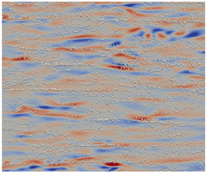
In this paper, we focus on Lagrangian particle tracking in WMLES. Figure 1 shows streamwise velocity contours on a plane cut through turbulent channel flow simulations using DNS and WMLES at a friction Reynolds number of  $Re_{\ast }=600$, highlighting the difference in resolution even at such a moderate Reynolds number. The WMLES captures large-scale motions in the flow, but lacks small-scale details which can be important for advecting inertial particles, particularly near the wall. These near-wall flow structures, however, may be vital for the accurate simulation of particle dynamics and turbophoresis (Marchioli & Soldati Reference Marchioli and Soldati2002). The challenge of predicting particle-laden flows using WMLES, therefore, is much more difficult than in WRLES, but WMLES is more practical for simulating high Reynolds number flows. Typically, the first grid point in WMLES lies outside the viscous and buffer layers, in the so-called logarithmic region of the flow. Therefore, the region of enhanced concentration due to turbophoresis is almost entirely within the first grid cell. Nonetheless, given the cost savings made possible by WMLES at higher Reynolds numbers, it is of high interest to investigate turbophoresis and particle concentration profiles in WMLES.

Figure 1. Streamwise velocity contours and sketch of typical mesh for (a) DNS with stretched mesh in the wall-normal direction and (b) WMLES with coarser uniform mesh.
The goal of this paper is to elucidate the physics of turbophoresis by analysing exact conservation equations, and to leverage the results to demonstrate the modelling challenges and opportunities for WMLES of particle-laden flows. In particular, we seek to clarify the level of detail needed in modelling the features of the fluid velocities seen by particles within one grid spacing of the boundary in WMLES. Of course, such an understanding must encompass different regimes of inertial particle behaviours, including variations with Stokes number and volume fraction effects. In order to focus on the physics of wall-bounded particle-laden flows, the simplest geometry, that of a flow between two flat plates, is studied.
The remainder of the paper is structured as follows. The problem set-up, governing equations and boundary conditions are described in § 2. The statistical consequences of exact conservation equations on turbophoresis and particle concentration profiles in a turbulent channel flow are analysed in § 3. In § 4, point-particle DNS (PP-DNS) is used to verify and quantify the analysis from the previous section. The insight gained from these two sections is used to devise a proof-of-concept model for WMLES in § 5, which performs better in certain regimes compared with others. Conclusions are then drawn in § 6.
2 Governing equations and problem set-up
This section introduces the governing equations and boundary conditions for particle-laden turbulent channel flow considered in this paper. The following sections analyse and present simulation methods and results for the scenario described here.
2.1 Turbulent channel flow
The fluid flow is described by velocity  $\boldsymbol{u}(\boldsymbol{x},t)$ and pressure
  $p(\boldsymbol{x},t)$ fields that evolve according to the incompressible Navier–Stokes equations,
 $$\begin{eqnarray}\displaystyle \unicode[STIX]{x2202}_{t}\boldsymbol{u}+(\boldsymbol{u}\boldsymbol{\cdot }\unicode[STIX]{x1D735})\boldsymbol{u}=-\unicode[STIX]{x1D735}(p/\unicode[STIX]{x1D70C}_{f})+\unicode[STIX]{x1D708}_{f}\unicode[STIX]{x1D6FB}^{2}\boldsymbol{u}+\boldsymbol{f},\quad \unicode[STIX]{x1D735}\boldsymbol{\cdot }\boldsymbol{u}=0, & & \displaystyle\end{eqnarray}$$
 where  $\unicode[STIX]{x1D70C}_{f}$ is the fluid mass density,
  $\unicode[STIX]{x1D708}_{f}$ is the kinematic viscosity and
  $\boldsymbol{f}$ signifies forcing by particles. The effect of including or neglecting the two-way coupling represented by
  $\boldsymbol{f}$ is documented in appendix D. For the mass fractions simulated in this paper, the two-way coupling is of secondary importance for the particle concentration profile compared with particle–particle collisions and so is neglected in the numerical calculations presented in the main body of the paper. Although the presence or absence of the two-way coupling does not change the form of the conservation expressions derived below for the particle phase, it is expected that it would quantitatively affect the drag force terms in those expressions when the mass fraction is sufficiently large.
For studying the physics of wall-bounded flows in the simplest case possible, this paper considers a turbulent channel flow. An imposed pressure gradient in the  $x$ (streamwise) direction,
  $\text{d}p/\text{d}x$, drives the flow and no-slip, no-penetration conditions are imposed at the (smooth) walls separated by a distance
  $2h$ in the
  $y$ (wall-normal) direction. Thus, the flow and particle statistics are homogeneous in the
  $x$ and
  $z$ (spanwise) directions in addition to the mirror symmetry about the centreline. A statistically stationary channel flow is characterized by the friction Reynolds number,
  $Re_{\ast }=u_{\ast }h/\unicode[STIX]{x1D708}_{f}$, where
  $u_{\ast }=\sqrt{-(\text{d}p/\text{d}x)h/\unicode[STIX]{x1D70C}_{f}}$ is the friction velocity. The smallest active scales in the flow are characterized by the friction length scale,
  $\unicode[STIX]{x1D6FF}_{\ast }=\unicode[STIX]{x1D708}_{f}/u_{\ast }$, and the friction time scale,
  $\unicode[STIX]{x1D70F}_{\ast }=\unicode[STIX]{x1D708}_{f}/u_{\ast }^{2}$.
2.2 Lagrangian particle tracking
The particle phase is described by  $N_{p}$ discrete particles with centre of mass
  $\boldsymbol{x}(t)$ and velocity
  $\boldsymbol{v}(t)$, evolving according to the trajectory equations,
 $$\begin{eqnarray}\displaystyle \dot{\boldsymbol{x}}^{(i)}=\boldsymbol{v}^{(i)},\quad \dot{\boldsymbol{v}}^{(i)}=\boldsymbol{a}^{(i)}(\boldsymbol{x},\boldsymbol{v}),\quad i=1,2,\ldots ,N_{p}, & & \displaystyle\end{eqnarray}$$
 where  $\boldsymbol{a}(\boldsymbol{x},\boldsymbol{v})$ is the acceleration of the particle due to fluid forces. Each spherical particle is characterized by its diameter (
 $d_{p}$) and mass density (
 $\unicode[STIX]{x1D70C}_{p}$). For small particles (
 $d_{p}<\unicode[STIX]{x1D6FF}_{\ast }$) at low particle slip Reynolds numbers (
 $Re_{p}=|\boldsymbol{u}-\boldsymbol{v}|d_{p}/\unicode[STIX]{x1D708}_{f}\ll 1$), Stokes drag can be used,
  $\boldsymbol{a}_{St}=(\boldsymbol{u}(\boldsymbol{x})-\boldsymbol{v})/\unicode[STIX]{x1D70F}_{p}$, with relaxation time
  $\unicode[STIX]{x1D70F}_{p}=\unicode[STIX]{x1D70C}_{p}d_{p}^{2}/(18\unicode[STIX]{x1D70C}_{f}\unicode[STIX]{x1D708}_{f})$ in the limit
  $\unicode[STIX]{x1D70C}_{p}\gg \unicode[STIX]{x1D70C}_{f}$. In DNS, the fluid velocity seen by the particle,
  $\boldsymbol{u}(\boldsymbol{x})$, must be interpolated from the Eulerian grid to particle locations for the drag law. In LES, the interpolated velocity only represents the filtered velocity seen by the particle. The remaining SGS velocity seen by the particles requires additional modelling (Fede et al. Reference Fede, Simonin, Villedieu and Squires2006; Kuerten Reference Kuerten2006; Marchioli et al. Reference Marchioli, Salvetti and Soldati2008b; Ray & Collins Reference Ray and Collins2014; Minier Reference Minier2015, Reference Minier2016; Marchioli Reference Marchioli2017; Park et al. Reference Park, Bassenne, Urzay and Moin2017). The simulations in this paper use the Schiller–Naumann drag,
  $\boldsymbol{a}_{SN}=\boldsymbol{a}_{St}(1+0.15Re_{p}^{0.687})$, which gives a finite Reynolds number correction (Schiller & Naumann Reference Schiller and Naumann1933; Balachandar & Eaton Reference Balachandar and Eaton2010). Note that the present work does not include a lift force, which could potentially play a role in the near-wall region where velocity gradients are largest. Simple lift models, such as the Saffman lift force, are not applicable here. Given the complexity and variety of lift models (Wang et al. Reference Wang, Squires, Chen and McLaughlin1997; Marchioli, Picciotto & Soldati Reference Marchioli, Picciotto and Soldati2007), we defer the effect of lift to future work.
At times within § 3, the Stokes drag form will be used to simplify expressions. The same procedures as shown below can also be performed using Schiller–Naumann drag to include finite Reynolds number correction terms. These expressions are used to generate the plots in this paper, to be consistent with the simulation, and are given in appendix A.
3 Analysis of particle statistics
In this section, equations for the evolution of particle statistics are derived and various moments (conservation equations) are considered. In addition to providing a framework for interpreting simulation results, a good amount of qualitative insight follows directly from the exact conservation equations. For instance, the power-law shape of particle concentration profiles in the viscous sublayer are shown to be a direct consequence of momentum conservation. Further, the power-law exponent can be formally bounded. Appendix B highlights that similar analysis can be performed for preferential concentration in homogeneous turbulence. The similarities between turbophoresis in wall-bounded flows and preferential concentration in homogeneous flows has been explored in other works as well (Bragg & Collins Reference Bragg and Collins2014; Sikovsky Reference Sikovsky2014).
3.1 Single-particle probability density function evolution
The particle ensemble has statistical homogeneity in the  $x$ and
  $z$ directions, so the particle statistics of interest include only wall-normal position and velocity. To this end, we study the single-particle position–velocity probability density function (PDF) defined by,
 $$\begin{eqnarray}\displaystyle f(y,v_{y};t)=\langle \unicode[STIX]{x1D6FF}(y-{\hat{y}}(t))\unicode[STIX]{x1D6FF}(v_{y}-\hat{v}_{y}(t))\rangle , & & \displaystyle\end{eqnarray}$$
 where  $\unicode[STIX]{x1D6FF}(x)$ is the Dirac delta function representing the fine-grained PDF. The angled brackets,
  $\langle \cdot \rangle$, are employed to denote ensemble averaging over a monodisperse system of particles. Practically speaking, these averages may be obtained by averaging over all identical particles in a given realization, as well as averaging in time. Such temporal averaging is more convenient for obtaining converged statistics from numerical simulations and is therefore used in subsequent sections.
For use with (3.1), the dynamics of each individual particle, equation (2.2), is projected in the wall-normal direction,
 $$\begin{eqnarray}\displaystyle \dot{{\hat{y}}}=\hat{v}_{y}\quad \dot{\hat{v}}_{y}=\hat{a}_{y}=\frac{u_{y}(\hat{\boldsymbol{x}},t)-\hat{v}_{y}}{\unicode[STIX]{x1D70F}_{p}}. & & \displaystyle\end{eqnarray}$$
 Differentiating (3.1) in time and substituting (3.2), one can obtain an evolution equation for  $f$,
$f$,
 $$\begin{eqnarray}\displaystyle \frac{\unicode[STIX]{x2202}f}{\unicode[STIX]{x2202}t}+\frac{\unicode[STIX]{x2202}(v_{y}f)}{\unicode[STIX]{x2202}y}+\frac{\unicode[STIX]{x2202}(\langle a_{y}|y,v_{y}\rangle f)}{\unicode[STIX]{x2202}v_{y}}={\dot{f}}_{coll}, & & \displaystyle\end{eqnarray}$$
 where the conditional average  $\langle a_{y}|y,v_{y}\rangle$ is shorthand for
  $\langle \hat{a}_{y}|{\hat{y}}=y,\hat{v}_{y}=v_{y}\rangle$, i.e. the average particle acceleration conditioned on wall-normal position and velocity. The right-hand side term,
  ${\dot{f}}_{coll}$, denotes the changes in particle velocity due to inter-particle collisions. Note that Sikovsky (Reference Sikovsky2014) starts from an equation similar to (3.3), but in that work the fluid velocity seen by the particle (which contributes to the acceleration term) is modelled by a stochastic forcing term. In this paper, no stochastic modelling assumptions are made about the fluid flow seen by the particle. Instead, the present analysis seeks to understand the consequences of the exact conservation equations for the particle phase.
3.2 Particle mass conservation
The particle number density (concentration) is obtained at any  $y$ location by integrating
  $f$ over all possible particle velocities,
 $$\begin{eqnarray}\displaystyle C(y;t)=C_{0}(t)\int _{-\infty }^{\infty }f(y,v_{y};t)\,\text{d}v_{y}, & & \displaystyle\end{eqnarray}$$
 where  $C_{0}(t)=\int C(y;t)\,\text{d}y$ is the bulk particle concentration. Integrating (3.3) over all velocities and multiplying by
  $C_{0}$, we obtain a mass conservation equation for the particle phase,
 $$\begin{eqnarray}\displaystyle \frac{\unicode[STIX]{x2202}C}{\unicode[STIX]{x2202}t}+\frac{\unicode[STIX]{x2202}(\langle v_{y}|y\rangle C)}{\unicode[STIX]{x2202}y}=0. & & \displaystyle\end{eqnarray}$$
 The collisional term exactly vanishes because each collision individually conserves mass. Assuming statistical stationarity,  $\unicode[STIX]{x2202}C/\unicode[STIX]{x2202}t=0$. It follows, then, that
  $\langle v_{y}|y\rangle =0$. This simply states that the net wall-normal flux of particles must vanish at all
  $y$ locations for the PDF to remain stationary in time.
3.3 Particle wall-normal momentum conservation
The particle wall-normal momentum, which is the same as the particle mass flux introduced in (3.5), is obtained as a first-order moment of  $f$,
$f$,
 $$\begin{eqnarray}\displaystyle \langle v_{y}|y\rangle C(y;t)=C_{0}\int _{-\infty }^{\infty }v_{y}f(y,v_{y};t)\,\text{d}v_{y}. & & \displaystyle\end{eqnarray}$$
 A conservation equation for the wall-normal momentum is obtained by multiplying (3.3) by  $C_{0}$ and
  $v_{y}$ and integrating over all particle velocities. The result is,
 $$\begin{eqnarray}\displaystyle \frac{\unicode[STIX]{x2202}(\langle v_{y}|y\rangle C)}{\unicode[STIX]{x2202}t}+\frac{\unicode[STIX]{x2202}(\langle v_{y}^{2}|y\rangle C)}{\unicode[STIX]{x2202}y}-\langle a_{y}|y\rangle C=0. & & \displaystyle\end{eqnarray}$$
 As with the mass conservation equation, the collisional term makes no contribution to the wall-normal momentum of the particle ensemble because each inter-particle collision individually conserves momentum. The third term on the left, the acceleration term, is obtained using integration by parts. At steady state,  $\unicode[STIX]{x2202}(\langle v_{y}|y\rangle C)/\unicode[STIX]{x2202}t=0$, and the particle wall-normal momentum balance reduces to,
 $$\begin{eqnarray}\displaystyle \frac{\text{d}}{\text{d}y}(\langle v_{y}^{2}|y\rangle C)=\langle a_{y}|y\rangle C. & & \displaystyle\end{eqnarray}$$
 Because  $\langle v_{y}|y\rangle =0$ from mass conservation,
  $\langle v_{y}^{2}|y\rangle$ represents the particle wall-normal velocity variance as a function of distance from the wall. This would not be the case for a spatially developing flow such as a turbulent boundary layer, in which case
  $\langle v_{y}^{2}|y\rangle$ could be split into mean-squared and variance components. Note that the derivative in
  $y$ on the left-hand side is now a total derivative since time dependence has been removed.
3.3.1 Mechanisms affecting non-uniform concentration
Using the product rule and assuming the Stokes drag formula,  $a_{y}=(u_{y}-v_{y})/\unicode[STIX]{x1D70F}_{p}$, the particle wall-normal momentum balance at steady state, equation (3.8), may be rewritten as,
 $$\begin{eqnarray}\displaystyle \langle v_{y}^{2}|y\rangle \frac{\text{d}C}{\text{d}y}=\left(\frac{\langle u_{y}|y\rangle }{\unicode[STIX]{x1D70F}_{p}}-\frac{\text{d}\langle v_{y}^{2}|y\rangle }{\text{d}y}\right)C. & & \displaystyle\end{eqnarray}$$
The two terms on the right-hand side, proportional to the local concentration level, must balance with the left-hand side term proportional to the concentration gradient. Thus, two mechanisms for generating non-uniform particle concentrations may be deduced from (3.9).

Figure 2. From a point-particle DNS snapshot of  $Re_{\ast }=150$ (details in § 4): location of
  $St^{+}=8$,
  $\unicode[STIX]{x1D6F7}_{V}=3\times 10^{-5}$ particles with centroid
  $5\leqslant y^{+}\leqslant 10$, white spheres, for particles superposed with contours at
  $y^{+}=10$ of the (a) streamwise velocity, (b) wall-normal velocity. The size of each particle is exaggerated for visualization purposes. The velocities are in friction units,
  $\boldsymbol{u}/u_{\ast }$.
The first right-hand side term in (3.9) represents the average drag force on the particles at a given distance from the wall. For Stokes drag, this is proportional to,  $\langle u_{y}|y\rangle$, the average wall-normal fluid velocity as sampled by particles at a given wall-normal location. In arriving at (3.9), it is recognized that the
  $\langle v_{y}|y\rangle$ contribution from the Stokes drag relation vanishes due to mass conservation, leaving only potential contributions from
  $\langle u_{y}|y\rangle$. For particles randomly distributed in the flow, this drag term vanishes. However, it is known that heavy particles tend to accumulate in low-speed streaks associated with ejection events in near-wall turbulence (Rashidi, Hetstroni & Banerjee Reference Rashidi, Hetstroni and Banerjee1990; Eaton & Fessler Reference Eaton and Fessler1994; Marchioli & Soldati Reference Marchioli and Soldati2002). Indeed, as shown in figure 2, the particles tend to prefer ‘ejection’ regions, which have lower streamwise velocity (
 $u_{x}^{\prime }<0$) and positive wall-normal velocity (
 $u_{y}^{\prime }>0$). As a result, the biased sampling term is positive (
 $\langle u_{y}|y\rangle >0$) near the wall as particles sample ejection events more often than sweeps. This means that the biased sampling provides a net force which pushes particles away from the wall.
The second term on the right-hand side is the turbophoresis pseudo-force, which creates the migration of particles down gradients in wall-normal velocity variance. The no-slip, no-penetration boundary conditions are enforced on the fluid phase at the wall, and the tendency of the particles to relax toward local fluid velocities will give lower  $\langle v_{y}^{2}|y\rangle$ in the immediate vicinity of the wall. This leads to
  $\text{d}\langle v_{y}^{2}|y\rangle /\text{d}y>0$, i.e. increasing particle wall-normal velocity fluctuations with increasing distance from the wall. As a result, turbophoresis causes a significant net migration of particles toward the wall which is only partially offset by the biased sampling force.
It is noteworthy that the analysis of Guha (Reference Guha1997, Reference Guha2008) has omitted the biased sampling term, but for low Stokes numbers, this term significantly affects the concentration profile. The difference between Eulerian-averaged fluid velocities and average fluid velocities seen by (non-randomly spaced) particles is included as a drift velocity in stochastic models (Minier, Chibbaro & Pope Reference Minier, Chibbaro and Pope2014). Near the wall, this drift velocity is driven by interaction with coherent structures, leading to the biased sampling effect of a net force away from the wall. The importance of this term will be further illustrated when considering the  $\unicode[STIX]{x1D70F}_{p}\rightarrow 0$ limit below. At higher Stokes numbers, the
  $\unicode[STIX]{x1D70F}_{p}$ in the denominator shows that the biased sampling force will diminish and likely become negligible compared to turbophoresis. The prediction of the turbophoresis force may not require detailed knowledge of particle interactions with turbulent coherent structures since it only relies on the gradient of particle wall-normal velocity variance. In contrast, turbulent coherent structures play a direct and unmistakable role in establishing the sampling bias term. For this reason, one objective of the numerical demonstrations below is to quantitatively assess at what Stokes number one may safely neglect the effect of the biased sampling term in (3.9) on the concentration profile, and hence potentially neglect the details of near-wall coherent structures. While turbophoresis and biased sampling are two distinct effects in the statistical equations, it should be appreciated that both naturally emerge from a true account of the particle dynamics in the presence of coherent structures (i.e. the fluid velocity seen by the particles), so they are not uncorrelated in a dynamical sense.
3.3.2 Formal solution
It is straightforward to construct the formal solution of (3.9),
 $$\begin{eqnarray}\displaystyle C(y)={\mathcal{N}}\exp \left(\underbrace{\frac{1}{\unicode[STIX]{x1D70F}_{p}}\int ^{y}\frac{\langle u_{y}|\unicode[STIX]{x1D702}\rangle }{\langle v_{y}^{2}|\unicode[STIX]{x1D702}\rangle }\,\text{d}\unicode[STIX]{x1D702}}_{\mathit{biased\,sampling}}-\underbrace{\int ^{y}\frac{\text{d}\ln \langle v_{y}^{2}|\unicode[STIX]{x1D702}\rangle }{\text{d}\unicode[STIX]{x1D702}}\,\text{d}\unicode[STIX]{x1D702}}_{\mathit{turbophoresis}}\right), & & \displaystyle\end{eqnarray}$$
 where  ${\mathcal{N}}$ is an integration constant which is unimportant for exploring causes of non-uniform concentration. Two phoresis integrals can be defined based on this form, as underscored in (3.10). The first phoresis integral,
 $$\begin{eqnarray}\displaystyle I_{bias}=\frac{1}{\unicode[STIX]{x1D70F}_{p}}\int _{0}^{y}\frac{\langle u_{y}|\unicode[STIX]{x1D702}\rangle }{\langle v_{y}^{2}|\unicode[STIX]{x1D702}\rangle }\,\text{d}\unicode[STIX]{x1D702}, & & \displaystyle\end{eqnarray}$$
 quantifies the effect of biased sampling on the resulting concentration profile. For positive  $\langle u_{y}|y\rangle$, this term alone would cause increasing concentration with increasing distance to the wall. Meanwhile, the second phoresis integral,
 $$\begin{eqnarray}\displaystyle I_{turb}=-\int _{0}^{y}\frac{\text{d}\ln \langle v_{y}^{2}|\unicode[STIX]{x1D702}\rangle }{\text{d}\unicode[STIX]{x1D702}}\,\text{d}\unicode[STIX]{x1D702}, & & \displaystyle\end{eqnarray}$$
 quantifies the influence of turbophoresis on the final concentration profile. In these two definitions, the wall location ( $y=0$) is used for the lower bound. These two definitions enable a straightforward, fair comparison of how biased sampling and turbophoresis affect the concentration profile and when one effect may be safely neglected. A relationship similar to (3.10) was considered by Capecelatro, Desjardins & Fox (Reference Capecelatro, Desjardins and Fox2016) in the context of two-fluid equations, but only after the biased sampling term was found to be negligible and removed from the analysis.
While (3.10) provides a formal expression for the concentration profile, it should be appreciated that it involves unclosed statistical terms depending, most notably, on the statistics of fluid velocities seen by particles at various wall-normal distances. At present, this expression is not necessarily advanced as a specific starting point for model development, but is rather used here to demonstrate qualitative features and provide a framework for elucidating the performance of models for the fluid velocities seen by particles.
3.3.3 The  $St\rightarrow \infty$ limit

Seeing that the turbophoresis integral, equation (3.12), may be formally integrated, then (3.10) may also be written as
 $$\begin{eqnarray}\displaystyle C(y)=\frac{{\mathcal{N}}}{\langle v_{y}^{2}|y\rangle }\exp \left(\frac{1}{\unicode[STIX]{x1D70F}_{p}}\int ^{y}\frac{\langle u_{y}|\unicode[STIX]{x1D702}\rangle }{\langle v_{y}^{2}|\unicode[STIX]{x1D702}\rangle }\,\text{d}\unicode[STIX]{x1D702}\right). & & \displaystyle\end{eqnarray}$$
 This form emphasizes that, at large Stokes numbers ( $\unicode[STIX]{x1D70F}_{p}^{-1}\rightarrow 0$) when the biased sampling becomes negligible, the concentration profile becomes inversely proportional to the wall-normal particle velocity variance. From a modelling perspective, this means that predicting concentration profiles for high Stokes number particles,
 $$\begin{eqnarray}\displaystyle C(y)\approx \frac{{\mathcal{N}}}{\langle v_{y}^{2}|y\rangle }, & & \displaystyle\end{eqnarray}$$
requires only an accurate representation of particle wall-normal velocity fluctuation magnitudes. The spatio-temporal details of interactions between particles and near-wall coherent structures becomes less important in this limit, simplifying the modelling task. In a WMLES simulation, it is possible to reproduce fairly accurate wall-normal velocity variances for the fluid (Bae et al. Reference Bae, Lozano-Durán, Bose and Moin2018) in the resolved region of the flow. However, it is less clear whether the variance profiles for particles, including Lagrangian sampling and memory effects, below the first grid point can be reproduced in the WMLES modelling approach.
3.3.4 The $St\rightarrow 0$ limit

In the opposite limit  $\unicode[STIX]{x1D70F}_{p}\rightarrow 0$, the particle velocity may be written as (Maxey Reference Maxey1987)
 $$\begin{eqnarray}\displaystyle v_{y}=u_{y}-\unicode[STIX]{x1D70F}_{p}\frac{\text{D}u_{y}}{\text{D}t}+O(\unicode[STIX]{x1D70F}_{p}^{2}). & & \displaystyle\end{eqnarray}$$
This means that the biased sampling force becomes
 $$\begin{eqnarray}\displaystyle \lim _{\unicode[STIX]{x1D70F}_{p}\rightarrow 0}\frac{\langle u_{y}|y\rangle }{\unicode[STIX]{x1D70F}_{p}}=\left\langle \frac{\text{D}u_{y}}{\text{D}t}\right\rangle =-\frac{1}{\unicode[STIX]{x1D70C}_{f}}\frac{\unicode[STIX]{x2202}\langle p\rangle }{\unicode[STIX]{x2202}y}. & & \displaystyle\end{eqnarray}$$
 Note that the viscous force,  $\unicode[STIX]{x1D708}_{f}\unicode[STIX]{x1D6FB}^{2}\langle u_{y}\rangle$, vanishes because
  $\langle u_{y}\rangle =0$ at steady state in the limit
  $\unicode[STIX]{x1D70F}_{p}\rightarrow 0$. At
  $\unicode[STIX]{x1D70F}_{p}=0$, the average over the particle ensemble becomes the same as the fluid ensemble average, the concentration profile becomes flat (incompressibility) and the wall-normal RANS equation is obtained from (3.9),
 $$\begin{eqnarray}\displaystyle 0=-\frac{\unicode[STIX]{x2202}\langle p\rangle }{\unicode[STIX]{x2202}y}+\frac{\text{d}\langle u_{y}^{2}\rangle }{\text{d}y}, & & \displaystyle\end{eqnarray}$$
 as in, for example, equation (5.2.2) of Tennekes & Lumley (Reference Tennekes and Lumley1972). This convergence of the  $\unicode[STIX]{x1D70F}_{p}\rightarrow 0$ limit of the biased sampling to the pressure gradient was previously pointed out in passing by Bragg & Collins (Reference Bragg and Collins2014) during a discussion of the analogy between preferential concentration in homogeneous turbulence and turbophoresis in wall-bounded turbulence. The approach to (3.17) illustrates that the sampling bias becomes equal and opposite to turbophoresis in small
  $St$ number limit, which highlights the importance of preferential sampling of near-wall structures at low Stokes numbers. This analysis confirms that accurately predicting the concentration profile of low Stokes number particles will require a much more detailed representation of the near-wall turbulent fluctuations than is present in WMLES. The numerical results in §§ 4 and 5 explore both low and high
  $St^{+}$ cases in more quantitative detail.
3.3.5 The $y\rightarrow 0$ limit

The above analysis may also be leveraged to demonstrate the existence of a power-law concentration profile in the viscous sublayer. The derivation stems from a low Stokes number expansion, but the reasons a power law can also be observed at higher Stokes numbers are discussed below. Consider (3.15) in the limit  $y\rightarrow 0$, where a Taylor expansion of the fluid velocity field prevails (i.e. in the viscous sublayer),
 $$\begin{eqnarray}\displaystyle \left.\begin{array}{@{}l@{}}u_{x}(x,y,z,t)=A_{x}(x,z,t)y+O(y^{2}),\\ u_{y}(x,y,z,t)=B_{y}(x,z,t)y^{2}+O(y^{3}),\\ u_{z}(x,y,z,t)=A_{z}(x,z,t)y+O(y^{2}).\end{array}\right\} & & \displaystyle\end{eqnarray}$$
 Note that the linear term  ${\sim}y$ for the wall-normal fluid velocity is exactly zero due to the divergence-free condition for incompressible flows (Kim, Moin & Moser Reference Kim, Moin and Moser1987; Pope Reference Pope2000). Substituting (3.18) into (3.15) for particles ‘almost’ following fluid trajectories, i.e.
 $$\begin{eqnarray}\displaystyle v_{y}=u_{y}-\unicode[STIX]{x1D70F}_{p}\left(\frac{\unicode[STIX]{x2202}u_{y}}{\unicode[STIX]{x2202}t}+u_{x}\frac{\unicode[STIX]{x2202}u_{y}}{\unicode[STIX]{x2202}x}+u_{y}\frac{\unicode[STIX]{x2202}u_{y}}{\unicode[STIX]{x2202}y}+u_{z}\frac{\unicode[STIX]{x2202}u_{y}}{\unicode[STIX]{x2202}z}\right)+O(\unicode[STIX]{x1D70F}_{p}^{2}), & & \displaystyle\end{eqnarray}$$
one obtains an expansion for the particle wall-normal velocities,
 $$\begin{eqnarray}\displaystyle v_{y}=A_{y}y^{2}-\unicode[STIX]{x1D70F}_{p}\left(y^{2}\frac{\unicode[STIX]{x2202}A_{y}}{\unicode[STIX]{x2202}t}+y^{3}A_{x}\frac{\unicode[STIX]{x2202}B_{y}}{\unicode[STIX]{x2202}x}+2y^{3}B_{y}^{2}+y^{3}A_{z}\frac{\unicode[STIX]{x2202}B_{y}}{\unicode[STIX]{x2202}z}\right)+O(\unicode[STIX]{x1D70F}_{p}^{2},y^{3}). & & \displaystyle\end{eqnarray}$$
From this expression, the particle wall-normal velocity variance can be assessed,
 $$\begin{eqnarray}\displaystyle \langle v_{y}^{2}|y\rangle =\underbrace{\langle A_{y}^{2}\rangle }_{\unicode[STIX]{x1D6FC}}y^{4}+O(\unicode[STIX]{x1D70F}_{p},y^{5}), & & \displaystyle\end{eqnarray}$$
 where statistically stationary flow has been assumed, i.e.  $\langle \unicode[STIX]{x2202}_{t}A_{y}\rangle =0$ and
  $\langle A_{y}\unicode[STIX]{x2202}_{t}A_{y}\rangle =0$. The biased sampling term can also be evaluated,
 $$\begin{eqnarray}\displaystyle \frac{\langle u_{y}|y\rangle }{\unicode[STIX]{x1D70F}_{p}}=\frac{\langle (u_{y}-v_{y})|y\rangle }{\unicode[STIX]{x1D70F}_{p}}=\underbrace{\left\langle A_{x}\frac{\unicode[STIX]{x2202}B_{y}}{\unicode[STIX]{x2202}x}+2B_{y}^{2}+A_{z}\frac{\unicode[STIX]{x2202}B_{y}}{\unicode[STIX]{x2202}z}\right\rangle }_{\unicode[STIX]{x1D6FD}}y^{3}+O(\unicode[STIX]{x1D70F}_{p},y^{4}). & & \displaystyle\end{eqnarray}$$
Together, equations (3.21) and (3.22) yield
 $$\begin{eqnarray}\displaystyle \left.\begin{array}{@{}l@{}}\langle v_{y}^{2}|y\rangle \approx \unicode[STIX]{x1D6FC}y^{4},\\ \langle u_{y}|y\rangle \approx \unicode[STIX]{x1D6FD}\unicode[STIX]{x1D70F}_{p}y^{3}.\end{array}\right\} & & \displaystyle\end{eqnarray}$$
 Although this has been derived specifically in the  $\unicode[STIX]{x1D70F}_{p}\rightarrow 0$ limit, it is reasonable to expect that the scalings in (3.23) hold over a decent range of finite Stokes numbers because the particle ensemble averages are biased toward particles with larger residence time in the near-wall region (trapped particles). These particles with longer residence times by definition have more time to adjust to the local near-wall fluid scalings. In fact, the numerical results below show that scalings for the particle velocity variance and biased sampling terms in (3.23) are observed over a generous range of Stokes numbers.
Substituting (3.23) into (3.13),
 $$\begin{eqnarray}\displaystyle C(y)=\frac{{\mathcal{N}}}{\unicode[STIX]{x1D6FC}y^{4}}\exp \left(\int ^{y}\frac{\unicode[STIX]{x1D6FD}\unicode[STIX]{x1D702}^{3}}{\unicode[STIX]{x1D6FC}\unicode[STIX]{x1D702}^{4}}\,\text{d}\unicode[STIX]{x1D702}\right)=\frac{{\mathcal{N}}}{\unicode[STIX]{x1D6FC}}y^{\unicode[STIX]{x1D6FD}/\unicode[STIX]{x1D6FC}-4}. & & \displaystyle\end{eqnarray}$$
 At  $\unicode[STIX]{x1D70F}_{p}=0$,
  $\unicode[STIX]{x1D6FD}=4\unicode[STIX]{x1D6FC}$ because the incompressibility of fluid particles implies a uniform concentration profile with biased sampling and turbophoresis balanced according to (3.17). For
  $\langle u_{y}|y\rangle$ to remain bounded as
  $\unicode[STIX]{x1D70F}_{p}$ becomes large, it must be that
  $\unicode[STIX]{x1D6FD}$ becomes small as Stokes number increases. (Note however that the expansion (3.20) will not apply at sufficiently high Stokes number.) At finite Stokes numbers, provided the near-wall scalings given by (3.23) hold,
  $0<\unicode[STIX]{x1D6FD}<4\unicode[STIX]{x1D6FC}$, then the concentration profile in the viscous sublayer has the form
 $$\begin{eqnarray}\displaystyle C(y)\sim y^{-\unicode[STIX]{x1D6FE}}, & & \displaystyle\end{eqnarray}$$
 with  $0<\unicode[STIX]{x1D6FE}<4$. Thus, the conservation of momentum in the wall-normal direction gives a simple understanding for near-wall power laws in particle concentration profiles, with power-law exponent bounded by
  $\unicode[STIX]{x1D6FE}<4$, provided the biased sampling coefficient
  $\unicode[STIX]{x1D6FD}$ behaves monotonically with
  $\unicode[STIX]{x1D70F}_{p}$ (this is confirmed in § 4). This bound is in agreement with previous stochastic models and observed DNS trends (Sikovsky Reference Sikovsky2014). As volume fraction increases, inter-particle collisions can interrupt this power-law behaviour by energizing near-wall particles and causing deviations from the
  $\langle v_{y}^{2}|y\rangle$ scaling in (3.23).
3.4 Higher-order moments
Higher-order moments,
 $$\begin{eqnarray}\displaystyle \langle v_{y}^{n}|y\rangle C(y;t)=C_{0}\int _{-\infty }^{\infty }v_{y}^{n}f(y,v_{y};t)\,\text{d}v_{y}, & & \displaystyle\end{eqnarray}$$
 can be analysed following the same procedure. The right-hand side term in (3.3) describing the effects of particle–particle collisions no longer vanishes exactly in the evolution equation for higher-order moments. For simplicity, then, only the zero volume fraction limit will be considered here. After explicitly neglecting collisional effects, the  $n$th moment of (3.3) gives
 $$\begin{eqnarray}\displaystyle \frac{\unicode[STIX]{x2202}(\langle v_{y}^{n}|y\rangle C)}{\unicode[STIX]{x2202}t}+\frac{\unicode[STIX]{x2202}(\langle v_{y}^{n+1}|y\rangle C)}{\unicode[STIX]{x2202}y}-n\langle a_{y}v_{y}^{n-1}|y\rangle C=0. & & \displaystyle\end{eqnarray}$$
At steady state for particles experiencing Stokes drag,
 $$\begin{eqnarray}\displaystyle \langle v_{y}^{n+1}|y\rangle \frac{\text{d}C}{\text{d}y}=\left(\frac{n}{\unicode[STIX]{x1D70F}_{p}}\langle (u_{y}-v_{y})v_{y}^{n-1}|y\rangle -\frac{\text{d}\langle v_{y}^{n+1}|y\rangle }{\text{d}y}\right)C, & & \displaystyle\end{eqnarray}$$
which has the formal solution
 $$\begin{eqnarray}\displaystyle C(y)=\frac{{\mathcal{N}}^{\prime }}{\langle v_{y}^{n+1}|y\rangle }\exp \left(\frac{n}{\unicode[STIX]{x1D70F}_{p}}\int ^{y}\frac{\langle (u_{y}-v_{y})v_{y}^{n-1}|\unicode[STIX]{x1D702}\rangle }{\langle v_{y}^{n+1}|\unicode[STIX]{x1D702}\rangle }\,\text{d}\unicode[STIX]{x1D702}\right). & & \displaystyle\end{eqnarray}$$
 Dividing this expression by (3.13) raised to the  $(n+1)/2$ power and rearranging yields,
 $$\begin{eqnarray}\displaystyle \frac{\langle v_{y}^{m}\rangle }{\langle v_{y}^{2}\rangle ^{m/2}}={\mathcal{N}}^{\prime \prime }C(y)^{m/2-1}\exp \left(\frac{m-1}{\unicode[STIX]{x1D70F}_{p}}\int ^{y}\frac{\langle (u_{y}-v_{y})v_{y}^{m-2}|\unicode[STIX]{x1D702}\rangle }{\langle v_{y}^{m}|\unicode[STIX]{x1D702}\rangle }\,\text{d}\unicode[STIX]{x1D702}-\frac{m}{2\unicode[STIX]{x1D70F}_{p}}\int ^{y}\frac{\langle u_{y}|\unicode[STIX]{x1D702}\rangle }{\langle v_{y}^{2}|\unicode[STIX]{x1D702}\rangle }\,\text{d}\unicode[STIX]{x1D702}\right), & & \displaystyle \nonumber\\ \displaystyle & & \displaystyle\end{eqnarray}$$
 where  $m=n+1$ has been substituted.
Therefore, when the concentration profile has a power law given by (3.25), and similar scaling arguments to those in § 3.3.5 hold, this expression gives a power law for the skewness, flatness, and other higher-order hyper-flatness values. In particular,
 $$\begin{eqnarray}\displaystyle \frac{\langle v_{y}^{m}\rangle }{\langle v_{y}^{2}\rangle ^{m/2}}\sim y^{-\unicode[STIX]{x1D6FE}(m/2-1)+\unicode[STIX]{x1D6FF}}, & & \displaystyle\end{eqnarray}$$
 where the  $\unicode[STIX]{x1D6FF}$ comes from the exponential term in (3.30) using (3.18) and (3.20) and following similar steps as before. Note that as
  $\unicode[STIX]{x1D70F}_{p}$ increases, this exponential term becomes small, leading to
  $\unicode[STIX]{x1D6FF}\rightarrow 0$ as
  $St$ becomes large. This limit is in agreement with the stochastic model of Sikovsky (Reference Sikovsky2014), namely, that flatness and hyper-flatness profiles have a power-law form near the wall with exponent
  $\unicode[STIX]{x1D6FE}(m/2-1)$. That model, however, apparently misses the correction term (
 $\unicode[STIX]{x1D6FF}$ in (3.31)) coming from the exponential term in (3.30), which is significant for smaller Stokes numbers. This is further apparent in the fact that their results for flatness,
  $m=4$, give better agreement at
  $St^{+}=25$ than at
  $St^{+}=5$.
4 Point-particle direct numerical simulation results
The previous section analysed conservation equations for the particle ensemble and obtained insightful but mostly qualitative results. This section now explores particle-laden turbulent channel flow numerically using the framework developed in the previous section. In particular, this section verifies the expectations enumerated above while providing quantitative results to complement many of these qualitative observations.
4.1 Numerical methods and simulation details
The continuum equations for the fluid, equation (2.1), are discretized on a staggered Cartesian grid, and second-order central differencing is employed. Trilinear interpolation is used to compute the flow quantities (e.g. velocity) at particle locations for the drag law, equation (2.2). While previous studies have recommended higher-order interpolation (Yeung & Pope Reference Yeung and Pope1988), we find that trilinear interpolation is sufficient for studying the concentration profile in this work, see appendix F. The Schiller–Naumann form,  $\boldsymbol{a}_{SN}$, is used for particle drag. In the present study, we consider the limit that
  $g\unicode[STIX]{x1D70F}_{p}/u_{\ast }$ is small, and thus neglect gravitational forces on the particles. The presence of a strong gravity force could alter the dynamics of the particles in a way that would depend on the orientation of the gravitational field with respect to the channel geometry. For instance, Lavezzo et al. (Reference Lavezzo, Soldati, Gerashchenko, Warhaft and Collins2010) found that acceleration statistics are significantly altered by gravity in the wall-normal direction.
A fractional step method for time advancement for the fluid and particles is done with Huen’s second-order method (RK2). Particle-particle collisions are computed using a hard-sphere collision model with a specified restitution coefficient. For this treatment, an efficient algorithm for detecting binary collisions using their collision cylinders within a given time step is implemented. The collision outcome is computed based on angle of incidence and the restitution coefficient. Unless otherwise given, a restitution coefficient of  $1$ is used (kinetic energy preserving collisions). Particle–wall collisions are similarly treated, with a unity restitution coefficient so that they conserve kinetic energy. The walls are considered smooth for both the continuum carrier fluid and for the particle–wall collisions, although it should be noted that wall roughness can play an important role (Sommerfeld Reference Sommerfeld1992; Kussin & Sommerfeld Reference Kussin and Sommerfeld2002; Benson, Tanaka & Eaton Reference Benson, Tanaka and Eaton2005; Vreman Reference Vreman2007; Konan, Simonin & Squires Reference Konan, Simonin and Squires2011; Milici et al. Reference Milici, De Marchis, Sardina and Napoli2014). Future work could extend this present study to consider rough walls or other effects such as adhesion.
The computational domain for the turbulent channel flow is periodic in  $x$ and
  $z$ with domain size
  $L_{x}=4\unicode[STIX]{x03C0}h$,
  $L_{y}=2h$, and
  $L_{z}=2\unicode[STIX]{x03C0}h$. The mean pressure gradient is imposed by a uniform body force to match the specified friction Reynolds number of
  $Re_{\ast }=u_{\ast }h/\unicode[STIX]{x1D708}$, where
  $u_{\ast }^{2}=-h(\text{d}p/\text{d}x)/\unicode[STIX]{x1D708}_{f}$ is the friction velocity. The results in this section are shown for
  $Re_{\ast }=150$, though appendix C shows equivalent results for
  $Re_{\ast }=300$ and
  $600$; the conclusions of this section hold for higher Reynolds numbers as well. The relative influence of particle inertia is represented by the friction Stokes number,
  $St^{+}=\unicode[STIX]{x1D70F}_{p}/\unicode[STIX]{x1D70F}_{\ast }=u_{\ast }^{2}\unicode[STIX]{x1D70F}_{p}/\unicode[STIX]{x1D708}$. When particle–particle collisions are considered, the other dimensionless parameter varied is the volume fraction,
  $\unicode[STIX]{x1D6F7}_{V}=\unicode[STIX]{x03C0}d_{p}^{3}N_{p}/(6L_{x}L_{y}L_{z})$, where
  $N_{p}$ is the total number of particles in the domain. The diameter of the particles is held constant at
  $d_{p}^{+}=0.5$ while the density ratio is changed to vary
  $St^{+}$. For some of the higher volume fractions shown in this section, the mass fraction is significant although two-way coupling effects are ignored. Appendix D explores two-way coupling effects and why neglecting them is justifiable in the present context. Further, appendix E explores the effect of restitution coefficient for particle–particle collisions. A restitution coefficient of
  $e=1.0$ is used for the results in this section.
The (DNS) grid resolution used in the homogeneous directions is  $\unicode[STIX]{x0394}x^{+}\approx 11$,
  $\unicode[STIX]{x0394}z^{+}\approx 7$. The grid is stretched in the wall-normal direction using a hyperbolic tangent to yield
  $\unicode[STIX]{x0394}y_{min}^{+}\approx 0.5$ for the first grid point at the wall (wall-parallel velocities at
  $y^{+}\approx 0.25$) and
  $\unicode[STIX]{x0394}y_{max}^{+}\approx 7$ in the centre of the channel. The resulting number of grid points was
  $172\times 86\times 128$ in the streamwise, wall-normal and spanwise directions, respectively. Sensitivity of the particle concentration profile to further refinement was explored and found to be small, so this grid resolution may be considered sufficient for the present purposes while keeping computational costs low. The particles are initialized with a uniform random distribution, and the simulation proceeds until the particles obtain a stationary distribution before statistics are computed. Aside from the cases shown in this paper, we also verified that the present numerical approach produced results consistent with the benchmark results from Marchioli et al. (Reference Marchioli, Soldati, Kuerten, Arcen, Tanière, Goldensoph, Squires, Cargnelutti and Portela2008c). Appendix F briefly explores the impact of grid resolution and interpolation scheme on the results of this section.
4.2 Simulation results without inter-particle collisions
Figure 3 shows the main results for the statistics of particle ensembles without inter-particle collisions at  $Re_{\ast }=150$ for a range of
  $0\leqslant St^{+}\leqslant 512$, using
  $d_{p}^{+}=0.5$ and varying the particle density
  $144\leqslant \unicode[STIX]{x1D70C}_{p}/\unicode[STIX]{x1D70C}_{f}\leqslant 36\,864$ to change
  $St^{+}$. The results from these particle ensembles represent the limit of
  $\unicode[STIX]{x1D6F7}_{V}\rightarrow 0$ since collisions are neglected. As can be seen from figure 3(a), in the absence of inter-particle collisions, the concentration near the wall can reach values hundreds of times larger than the mean concentration level. The concentration profiles are computed on a uniform grid with spacing of
  $0.5\unicode[STIX]{x1D6FF}_{\ast }$. Note that the
  $St^{+}=0$ tracer particles have a flat distribution with slight interpolation and time discretization errors leading to an almost imperceptibly reduced concentration in the viscous sublayer.

Figure 3. Particles statistics from turbulent channel flow at  $Re_{\ast }=150$ in the zero volume fraction limit (no inter-particle collisions) at various Stokes numbers: (a) concentration profiles; (b) root-mean-square wall-normal particle velocity, where the dashed grey curve indicates
  $v_{y}\sim y^{2}$ asymptotic behaviour near the wall; (c) sampling bias
  $\langle u_{y}|y\rangle$ for the particle ensembles with dashed grey line indicating
  ${\sim}y^{3}$ behaviour near the wall; (d) sampling bias and turbophoresis integrals, see (3.11) and (3.12).
The particle root-mean-square velocity fluctuations,  $v_{y,rms}=\sqrt{\langle v_{y}^{2}|y\rangle }$, shown in figure 3(b) reveal that the asymptotic
  $v_{y}\sim y^{2}$ behaviour near the wall persists even up to relatively high
  $St^{+}$. Meanwhile, figure 3(c) shows the sampling bias term
  $\langle u_{y}|y\rangle$, demonstrating that the
  ${\sim}y^{3}$ behaviour of that term also extends to relatively large values of
  $St^{+}$. Taken together, these two figures justify the scaling behaviour, equation (3.23), used in § 3.3.5 well outside of the
  $St^{+}\ll 1$ range. Further investigation into this observation (not shown) elucidates that this happens because particle statistics near the wall are dominated by trapped particles with long enough residence times to adjust to viscous sublayer fluid fluctuations despite nominally large
  $St^{+}$.
The resulting phoresis integrals, equations (3.11) and (3.12), are shown in figure 3(d). The integrals are both positive in all cases and are computed on a uniform grid with spacing  $0.5\unicode[STIX]{x1D6FF}_{\ast }$ using a trapezoidal rule integration. The exponential of their difference is the concentration profile, as verified in figure 4. At
  $St^{+}=2$, the sampling bias term mostly cancels the turbophoresis term. As the Stokes number is increased, however, the sampling bias term decreases sharply, leading to the more extreme near-wall enhancements of the concentration profile seen in figure 3. At a large enough Stokes number, say
  $St^{+}\geqslant 128$, the sampling bias integral is negligible compared to the turbophoresis integral, showing that the concentration profile is simply inversely proportional to the particle velocity variance as in (3.14). It should be noted, however, that for these high Stokes numbers, the particle wall-normal velocity variance deviates significantly from that of the fluid at any given distance from the wall. Therefore, it is still non-trivial that a WMLES designed to reproduce fluid velocity variances in the near-wall region would necessarily produce accurate particle velocity variances and concentration profiles, even in the high Stokes number limit.


For completeness, equation (3.10) for the concentration profile is directly verified by comparing left and right sides in figure 4(a). In figure 4(b), the same comparison is done using (3.14) instead, i.e. neglecting the sampling bias effect. This further emphasizes that for  $St^{+}\geqslant 128$, the details of the interactions between particles and turbulent structures near the wall are not as important. Instead, the concentration profile can be predicted with good accuracy simply by the inverse of the particle wall-normal velocity variance.
4.3 Simulation results with inter-particle collisions
In the near-wall region, the combination of higher local volume fractions due to turbophoresis with sharp flow gradients enhances the role of inter-particle collisions even at relatively modest bulk volume fractions (Kuerten & Vreman Reference Kuerten and Vreman2015). Inter-particle collisions, therefore, become non-negligible at much lower bulk volume fractions in wall-bounded flows compared to what one might expect using traditional heuristics which do not consider the near-wall region (Elghobashi Reference Elghobashi1994). The main effect of the collisions is to reduce the near-wall concentration levels by flattening the wall-normal fluctuation profiles (Li et al. Reference Li, McLaughlin, Kontomaris and Portela2001; Yamamoto et al. Reference Yamamoto, Potthoff, Tanaka, Kajishima and Tsuji2001). Caraman, Borée & Simonin (Reference Caraman, Borée and Simonin2003) emphasized that particle–particle collisions enhance the wall-normal transport of particles by transfer of streamwise fluctuation energy into wall-normal fluctuations. Because of turbophoresis and enhanced relative velocities, most particle–particle collisions happen very close to the wall (Kuerten & Vreman Reference Kuerten and Vreman2016). As volume fraction increases, inter-particle collisions tend to bring the concentration profile toward a uniform profile, attenuating the effects of turbophoresis. Point-particle methods, therefore, must account for inter-particle collisions to produce accurate concentration profiles.

Figure 5. Statistics for  $St^{+}=32$ particles in a turbulent channel flow at
  $Re_{\ast }=150$ at various volume fractions. Descriptions of panels are the same as in figure 3.
Figure 5 shows the same results as figure 3, but for particle ensembles including inter-particle collisions. For brevity, only  $St^{+}=32$ is shown (
 $\unicode[STIX]{x1D70C}_{p}/\unicode[STIX]{x1D70C}_{f}=2304$), although the main observations made here apply to other Stokes numbers as well. The most striking observation to be made from figure 5(a) is that the enhanced concentration near the wall due to turbophoresis is suppressed by the effect of inter-particle collisions even at seemingly innocuous bulk volume fractions. With volume fraction increased to
  $\unicode[STIX]{x1D6F7}_{V}=10^{-4}$, the peak concentration profile at the wall is less than five times the bulk concentration. At the highest volume fraction, the mass fraction is certainly appreciable, but it is shown in appendix D that the two-way coupling force does not strongly impact the concentration profile compared to the particle–particle collisions for the volume fractions considered here. Other quantities such as turbulence modulation or particle acceleration statistics may be more sensitive to the two-way coupling force, but we do not consider these at the present. Collisional effects on the concentration profile are seen even for volume fractions as low as
  $\unicode[STIX]{x1D6F7}_{V}=10^{-6}$.
The main cause of this change is demonstrated in figure 5(b), where the particle wall-normal fluctuations near the wall increase dramatically above the fluid fluctuation levels as volume fraction is increased. The increased levels of fluctuation can be attributed to a more ballistic behaviour of particles as they collide more frequently and redistribute streamwise fluctuations into wall-normal fluctuations. This also impacts the sampling bias, as shown in figure 5(c). However, in terms of the resulting concentration profile, the dominant effect of collisions is the decrease in the turbophoresis integral, figure 5(d), leading to the decreased near wall (relative) concentration. The increased fluctuations near the wall, far in excess of local fluid fluctuation levels, break the scaling behaviours of (3.23) which are responsible for the near-wall power law in concentration. In fact, figure 5 shows that the concentration profiles for higher volume fraction cases no longer display convincing power laws near the wall. It is also apparent from figure 5(d) that the biased sampling effect is also significantly attenuated by particle–particle collisions as volume fraction increases. This may be attributed to the enhanced collision rates limiting the tendency of particles to preferentially concentrate in low-speed streaks (figure 2).
The verification of (3.10) is included in figure 6(a) for the cases with inter-particle collisions. The conservation of momentum by particle collisions ensures that the  ${\dot{f}}_{coll}$ term does not contribute, and (3.13) accurately describes the concentration profiles in both cases. As the volume fraction increases, the sampling bias integral becomes more negligible compared to the turbophoresis integral, meaning that the higher volume fraction cases have concentration profiles very close to the inverse of their wall-normal particle velocity variance profiles, equation (3.14).


5 Wall-modelled large-eddy simulation results
The DNS results in the previous section included sufficient grid resolution to capture all the flow structures in the near-wall region. At higher Reynolds numbers, the computational cost of DNS or even WRLES becomes very steep, motivating the consideration of WMLES. With this in mind, this section explores the transport of particles in a WMLES framework.
5.1 Modelling and simulation details
The friction Reynolds number for the simulations in this section is  $Re_{\ast }=600$, which is high enough for WMLES to make sense while keeping the cost of DNS at a reasonable level. The number of grid points in each direction for the DNS is
  $682\times 342\times 512$, in keeping with the grid spacings given in the previous section. The WMLES grid is just
  $128\times 20\times 96$, a reduction by a factor of almost
  $500$. Unlike the DNS grid described in the previous section, the WMLES grid has uniform spacing in the wall-normal direction, so the first grid point is at
  $y_{1}^{+}=60$ for the wall-normal velocities and at
  $y_{1/2}^{+}=30$ for the streamwise and spanwise velocities. The details of the discretization are the same, but the WMLES solves the filtered Navier–Stokes equations,
 $$\begin{eqnarray}\displaystyle \unicode[STIX]{x2202}_{t}\widetilde{\boldsymbol{u}}+\widetilde{\boldsymbol{u}}\boldsymbol{\cdot }\unicode[STIX]{x1D735}\widetilde{\boldsymbol{u}}=-\frac{1}{\unicode[STIX]{x1D70C}_{f}}\unicode[STIX]{x1D735}\widetilde{p}+\unicode[STIX]{x1D708}_{f}\unicode[STIX]{x1D6FB}^{2}\widetilde{\boldsymbol{u}}-\unicode[STIX]{x1D735}\boldsymbol{\cdot }\unicode[STIX]{x1D748}, & & \displaystyle\end{eqnarray}$$
 where  $\unicode[STIX]{x1D70E}_{ij}=\widetilde{u_{i}u_{j}}-\widetilde{u}_{i}\widetilde{u}_{j}$ is the subgrid stress tensor computed using the dynamic Smagorinsky model (Germano et al. Reference Germano, Piomelli, Moin and Cabot1991), where the dynamic constant is found using the least-squares approximation of Lilly (Reference Lilly1992). The algebraic equilibrium wall model is used in lieu of the no-slip condition because the wall is not resolved. This wall model computes the wall shear stress locally (at each wall-adjacent grid point) from,
 $$\begin{eqnarray}\displaystyle u_{\Vert }(y_{1/2})=u_{\ast }\left[\frac{1}{\unicode[STIX]{x1D705}}\ln \left(\frac{y_{1/2}u_{\ast }}{\unicode[STIX]{x1D708}_{f}}\right)+B\right], & & \displaystyle\end{eqnarray}$$
 using the wall-parallel velocity magnitude,  $u_{\Vert }(y_{1/2})=\sqrt{u_{x}^{2}+u_{z}^{2}}$, at the first grid point,
  $y_{1/2}$, to find
  $\unicode[STIX]{x1D70F}_{w}=\unicode[STIX]{x1D70C}_{f}u_{\ast }^{2}$ via Newton iterations. Constants
  $\unicode[STIX]{x1D705}=0.41$ and
  $B=5.2$ are used. The coarse-grained WMLES velocity field captures the large-scale motions and mean flow, but is lacking small-scale features throughout the channel, most critically below the first grid point,
  $y<y_{1/2}$, where much of the physics related to biased sampling occurs.
The discretization schemes for WMLES are the same as the DNS described above. The same equations for advancing particle trajectories are used, equation (2.2), but with the filtered velocity,  $\widetilde{\boldsymbol{u}}$, used for the fluid velocity seen by the particle instead of the (unknown) full velocity,
  $\boldsymbol{u}$. While deconvolution schemes for approximately reconstructing
  $\boldsymbol{u}$ from
  $\widetilde{\boldsymbol{u}}$ (Kuerten Reference Kuerten2006) may work well with WRLES, it is unlikely to produce significant improvements in WMLES because of the much more severe lack of resolution in the near-wall region. Instead, no attempt is presently made to model the SGS velocity fluctuations (as seen by the particle) in the near-wall region. The Smagorinsky subgrid stress model that is used does imply subgrid fluctuations, so in that sense, the fluid velocity seen by the particles is not fully consistent with the fluid momentum equation solved (Minier Reference Minier2016). Nevertheless, the purpose of this investigation is to first focus on how the velocity seen by the particle can be interpolated from the first grid point off the wall, seeing that standard linear or higher-order interpolation schemes assume the flow variation is captured on the grid. Particle–particle collisions are computed deterministically using the same hard-sphere collision model so that the impact of volume fraction,
  $\unicode[STIX]{x1D6F7}_{V}$, can be demonstrated as well. The particle dynamics has no stochastic input, and so remains deterministic as in the case of DNS.
In the general case, it should be appreciated that the lack of subgrid fluctuations in the present WMLES approach can impact the collision rates predicted by the simulation. The collision cylinder approach used at present is based on smooth particle trajectories within a given time step. Additional sub time step variation in the trajectory (e.g. from a stochastic model) could change the collision rate, most likely increasing it. For the case of inertialess particle–wall collisions in a stochastic modelling framework, Dreeben & Pope (Reference Dreeben and Pope1998) proposed a method for dealing with this effect. Henry et al. (Reference Henry, Minier, Mohaupt, Profeta, Pozorski and Tanière2014) proposed a model for collisions between inertial particles in a stochastic framework. In the present work, because of the relatively moderate  $Re_{\unicode[STIX]{x1D70F}}$ (time-scale separation) along with the
  $St^{+}\gg 1$ values used,
  $\unicode[STIX]{x0394}t_{WMLES}/\unicode[STIX]{x1D70F}_{p}\ll 1$ so that these effects are not crucial at present.
5.2 Interpolation near the wall
While no attempt is made in the WMLES cases to model subgrid coherent structures, the interpolation scheme can have an important impact on the results. The baseline interpolation scheme is simply the trilinear interpolation used in DNS, which is consistent with a no-slip boundary condition. Because the viscous and buffer layers are not resolved by the WMLES, even the mean streamwise velocity seen by the particles below the first grid point is not well represented by linear interpolation. For that reason, a wall-parallel velocity interpolation consistent with the equilibrium stress model, denoted by  ${\mathcal{I}}_{\Vert }$, is developed. This interpolation scheme computes the wall-parallel velocity at a particle location as,
 $$\begin{eqnarray}\displaystyle \widetilde{u}_{\Vert }(y_{p})=F_{\Vert }(y^{+})\widetilde{u}_{\Vert }(y_{1/2}), & & \displaystyle\end{eqnarray}$$
 where  $F_{\Vert }(y^{+})=\langle u_{x}\rangle (y_{p}^{+})/\langle u_{x}\rangle (y_{1/2}^{+})$ is specified for the present purposes by a universal velocity profile from Liakopoulos (Reference Liakopoulos1984) which reproduces viscous, buffer, and log-law layers of a typical turbulent wall-bounded flow. An equivalent model could solve the RANS equations on a one-dimensional (1-D) grid below the first grid point, as often done for the equilibrium stress model (Cabot & Moin Reference Cabot and Moin2000; Bose & Park Reference Bose and Park2018), and use this velocity to advect particles.
Furthermore, the analysis in § 3 showed that the concentration profile for high Stokes number particles could potentially be predicted without knowledge of the details of near wall flow structures, provided that the profile of wall-normal velocity variance is accurately represented. To test this idea, the linear interpolation of the wall-normal velocity can be replaced by a more detailed interpolation scheme, denoted by  ${\mathcal{I}}_{\bot }$, which is designed to reproduce a realistic profile of wall-normal fluid velocity variance. To do this, the vertical velocity at a particle location is interpolated using,
 $$\begin{eqnarray}\displaystyle \widetilde{u}_{\bot }(y_{p})=F_{\bot }(y^{+})\widetilde{u}_{\bot }(y_{1}), & & \displaystyle\end{eqnarray}$$
 where  $F_{\bot }(y^{+})=\sqrt{\langle u_{\bot }^{\prime 2}\rangle }(y_{p})/\sqrt{\langle u_{\bot }^{\prime 2}\rangle }(y_{1})$ is given by a wall-normal velocity root-mean-square profile. For the present work, this profile was simply extracted from DNS and fitted with a sixth-order polynomial function with a
  $0.9\,\%$ relative error with respect to the DNS profile. This strategy (
 ${\mathcal{I}}_{\bot }$) enforces the right profile of the sampled wall-normal fluid velocity variance that the particles experience near the wall. As with the Liakopoulos profile, this approach is chosen for simplicity of implementation, since this work is viewed more as a conceptual test rather than as a specific modelling proposal. One could imagine constructing
  $F_{\bot }(y^{+})$ by using an existing Reynolds stress transport (Durbin Reference Durbin1993) or
  $v^{2}-f$ (Durbin Reference Durbin1991) model to solve for
  $\langle u_{\bot }^{\prime 2}\rangle$ on a 1-D grid similar to what is done for the mean velocity in equilibrium wall models. Pursuing the details and implementation of the model is beyond the scope of the present work, rather we seek to demonstrate how well such a model could be expected to perform.
5.3 Results
In this section, the results from three different WMLES variants are compared with DNS in terms of particle statistics. Since the underlying particle model is not changed between cases, this comparison highlights the impact of coarse resolution of the turbulent flow on the particle dynamics in WMLES. Since particular attention is given to the mean concentration profile, the effects of biased sampling and turbophoresis are highlighted.

Figure 7. Mean streamwise fluid velocity as sampled by the particle ensembles at (a,b)  $St^{+}=8$ and (c,d)
  $St^{+}=128$. Results at two volume fractions are shown: (a,c)
  $\unicode[STIX]{x1D6F7}_{V}=1\times 10^{-6}$ and (b,d)
  $\unicode[STIX]{x1D6F7}_{V}=1\times 10^{-5}$. In all panels, the dashed grey line indicates the log-law profile
  $u^{+}=\unicode[STIX]{x1D705}^{-1}\ln (y^{+})+B$ and the dotted grey line shows the viscous sublayer profile
  $u^{+}=y^{+}$. The vertical dash-dot lines indicate the location of the first
  $u_{x}$ grid point at
  $y_{1/2}^{+}=30$. The WMLES–
 ${\mathcal{I}}_{\Vert }$ and WMLES–
 ${\mathcal{I}}_{\Vert }$,
  ${\mathcal{I}}_{\bot }$ results are virtually indistinguishable.
One of the effects of biased sampling is that particles tend to preferentially sample the low-speed streaks in the buffer layer. As a result,  $\langle u_{x}|y\rangle$ for the particle ensemble will tend to be slower than the mean flow velocity using Eulerian averaging. That is, on average, particles at a given distance from the wall tend to move more slowly in the streamwise direction compared to the mean fluid velocity at the wall-normal location. As a result, streamwise particle velocities will be over-predicted in a WMLES–
 ${\mathcal{I}}_{\Vert }$ where buffer layer structures are largely absent but the mean velocity profile takes into account the law of the wall. This is shown in figure 7. Without the
  ${\mathcal{I}}_{\Vert }$ interpolation, simple trilinear interpolation under-predicts the mean flow velocity below the first grid point leading to an under-prediction of particle velocities as well. The effect of biased sampling is stronger at
  $St^{+}=8$ than
  $St^{+}=128$, as indicated by larger discrepancy between the DNS results and the WMLES–
 ${\mathcal{I}}_{\Vert }$ results (which follow closely the
  $u^{+}=y^{+}$ relation in the viscous sublayer). There is no noticeable effect of changing
  $\unicode[STIX]{x1D6F7}_{V}$, so particle–particle collisions seems to have a negligible impact here.

Figure 8. Particle wall-normal velocity fluctuation magnitudes as a function of distance from the wall at (a,b)  $St^{+}=8$ and (c,d)
  $St^{+}=128$. Results at two volume fractions are shown: (a,c)
  $\unicode[STIX]{x1D6F7}_{V}=1\times 10^{-6}$ and (b,d)
  $\unicode[STIX]{x1D6F7}_{V}=1\times 10^{-5}$. In all panels, the dashed grey line represents
  $u_{y}\sim y^{2}$ behaviour expected from the fluid velocity. The vertical dash-dot lines indicate the location of the first
  $u_{y}$ grid point at
  $y_{1}^{+}=60$. Significant particle slip and particle–particle collision effects prevent the particle velocity from following that scaling. The
  ${\mathcal{I}}_{\bot }$ interpolation scheme significantly improves the WMLES results.
While the  ${\mathcal{I}}_{\Vert }$ interpolation is designed to improve the streamwise fluid velocities below the first grid point, § 3 showed that turbophoresis is driven by the variance of (particle) wall-normal velocities. The interpolation based on fluid wall-normal velocity variance profiles,
  ${\mathcal{I}}_{\bot }$, is designed to address this facet. Figure 8 demonstrates the improved particle velocity variance profiles achieved using WMLES–
 ${\mathcal{I}}_{\Vert }$,
  ${\mathcal{I}}_{\bot }$. While improving the fluid variance profiles certainly helps, it by no means guarantees accurate particle variance profiles, since how particles sample the flow also impacts their velocity variance. Furthermore, particle–particle collisions can also change the variance profiles, particularly close to the wall as shown in figure 5(b). The profiles of particle wall-normal velocity fluctuations are shown in figure 8 for the same four cases shown in figure 7. In particular, the effect of
  ${\mathcal{I}}_{\bot }$ in generating better agreement with DNS is demonstrated for all four cases. Some discrepancy is still observed, particularly very close to the wall in the
  $St^{+}=128$ cases, because the higher inertia leads to a stronger tendency for the particles to deviate from local fluid velocities.

Figure 9. Biased sampling (3.11) and turbophoresis integrals (3.12) at (a,b)  $St^{+}=8$ and (c,d)
  $St^{+}=128$. Results at two volume fractions are shown: (a,c)
  $\unicode[STIX]{x1D6F7}_{V}=1\times 10^{-6}$ and (b,d)
  $\unicode[STIX]{x1D6F7}_{V}=1\times 10^{-5}$. The biased sampling term is poorly predicted by WMLES in all cases, but this term is more negligible in the
  $St^{+}=128$ case.
The competing effects of biased sampling and turbophoresis are shown in figure 9 for both DNS and the three WMLES approaches. The logarithmic scale highlights the discrepancies between DNS and WMLES in terms of biased sampling, since the WMLES does not contain the near-wall structures which dominate this effect. Instead the biased sampling is much smaller in WMLES, particularly below the first WMLES grid point where it even becomes negative for some  $y^{+}$ values (only the positive branch is shown in the plot). The DNS results show that the biased sampling is approximately one order of magnitude smaller for the
  $St^{+}=128$ cases compared to the
  $St^{+}=8$ cases. This means that the (absolute) error made in WMLES with the biased sampling is more negligible in the higher Stokes number cases, as expected.

Figure 10. Particle concentration profiles at (a,b)  $St^{+}=8$ and (c,d)
  $St^{+}=128$. Results at two volume fractions are shown: (a,c)
  $\unicode[STIX]{x1D6F7}_{V}=1\times 10^{-6}$ and (b,d)
  $\unicode[STIX]{x1D6F7}_{V}=1\times 10^{-5}$. Changes to the interpolation do not significantly help WMLES accuracy at
  $St^{+}=8$ but significant improvements can be seen for
  $St^{+}=128$.
The concentration profiles in figure 10 can be viewed as the exponential of the difference between the two phoresis integrals in figure 9, see (3.10). From the results in figure 10(a,b), it is clear that the enhanced interpolation methods provide no benefit at  $St^{+}=8$ in obtaining accurate concentration profiles in WMLES. This is because, while the turbophoresis may be more accurately represented due to a better wall-normal velocity variance profile, the biased sampling is very influential at low Stokes numbers. Without substantial enrichment of near-wall turbulent structures, biased sampling cannot be predicted well by WMLES. At higher Stokes numbers, figure 10(c,d) demonstrates that this is less pressing. The WMLES–
 ${\mathcal{I}}_{\Vert }$,
  ${\mathcal{I}}_{\bot }$ model reproduces the fluid wall-normal velocity variance, but some discrepancies exist in the particle wall-normal velocity which means that there are still remaining discrepancies in the predicted concentration profile at
  $St^{+}=128$, even when biased sampling becomes negligible. This occurs partly because the fluid fluctuations below the first grid point, while having a corrected magnitude, are essentially slaved to the fluctuations at the first grid point (
 $60$ viscous units in this case) rather than having their own unique small-scale signature.
6 Conclusions
This paper demonstrates that many of the features known about particle concentration profiles in wall-bounded turbulence can be understood simply by considering the implications of wall-normal momentum conservation for the particle phase, without any stochastic modelling assumptions. In particular, the balance equation for wall-normal particle momentum in a turbulent channel flow can be formally solved for the non-uniform concentration profile in terms of turbophoresis and biased sampling contributions, here referred to as phoresis integrals. Analysis of the  $y\rightarrow 0$ limit (viscous sublayer) provides straightforward reasoning, without stochastic modelling assumptions, for the existence of a power-law shape to the near-wall concentration profile at low volume fractions. This observation brings clarity to the underlying reason that concentration profiles have been observed to have power-law behaviours near the wall over a range of Stokes numbers. However, particle–particle collisions break the scalings as volume fraction is increased owing to the higher fluctuation levels near the wall that deviate from the asymptotic behaviour of fluid fluctuations. In the absence of significant collisional effects, further results such as related near-wall power laws for particle velocity skewness and flatness are also derived directly from the analysis, including low
  $St^{+}$ correction to the stochastic modelling results of Sikovsky (Reference Sikovsky2014).
Although the turbophoresis pseudo-force has been known and explored in many previous theoretical studies (Caporaloni et al. Reference Caporaloni, Tampieri, Trombetti and Vittori1975; Reeks Reference Reeks1983; Guha Reference Guha1997), the biased sampling term has not received the same attention. In some cases, it is (presumably) absorbed into a stochastic model (Sikovsky Reference Sikovsky2014) and in other cases it has been simply neglected (Guha Reference Guha1997, Reference Guha2008). Stochastic models for the fluid velocity seen by particles have recognized the importance of this effect as a drift velocity (Minier et al. Reference Minier, Chibbaro and Pope2014), and the results of this study may help guide or assess further developments in that modelling framework. Physically speaking, the tendency of inertial particles to preferentially accumulate in ejection events leads to a net force on the particle ensemble away from the wall, which mitigates the effect of turbophoresis on the near-wall concentration, particularly at small and moderate  $St^{+}$ values. Previous numerical studies have focused on how near-wall coherent structures influence turbophoresis (Marchioli & Soldati Reference Marchioli and Soldati2002) and developed simplified models for particle interactions with coherent structures which do not include biased sampling effects (Guingo & Minier Reference Guingo and Minier2008; Jin et al. Reference Jin, Potts and Reeks2015). The analysis here reveals that these small-scale flow structures are more directly influential through the biased sampling term.
On the other hand, the results in this paper do show that biased sampling becomes less important at high Stokes numbers ( $St^{+}\gtrsim 100$), leading to a concentration profile that is inversely proportional to the particle wall-normal velocity variance. While in the infinite Stokes number limit, the wall-normal velocity variance profile should become uniform, effectively eliminating the turbophoresis effect, we find that near-wall particle fluctuations are still significantly reduced up to
  $St^{+}=512$. Therefore, a range of
  $St^{+}$ is observed for which turbophoresis is still active but biased sampling is rather negligible. This has potentially important consequences for WMLES, which in the high
  $St^{+}$ regime may only require accurate fluctuation intensity profiles and likely need not recover the spatio-temporal details of interactions between particles and near-wall turbulent structures. Tests of this hypothesis using a DNS-tuned interpolation kernel below the first grid point showed that it is possible to obtain improved concentration profiles using this approach. However, the details of the near-wall structures still matter in a secondary way due to the mismatch between fluid and particle fluctuation intensities near the wall at high
  $St^{+}$. On the other hand, as can be seen from the analysis, simply producing correct wall-normal velocity variance profiles is not a viable approach at lower
  $St^{+}$. This is because such an approach ignores the biased sampling effect predominantly caused by flow structures unresolved by WMLES. This effect cannot be imparted in WMLES simply by changing the interpolation kernel near the wall. Instead, further work is required to provide an efficient method of enriching WMLES with small-scale information representative of these near-wall coherent structures. One possible direction could be the use of multi-scale ‘inner–outer’ simulation approaches (Pascarelli, Piomelli & Candler Reference Pascarelli, Piomelli and Candler2000; Tang & Akhavan Reference Tang and Akhavan2016; Sandham, Johnstone & Jacobs Reference Sandham, Johnstone and Jacobs2017).
Acknowledgements
This investigation was funded by the Advanced Simulation and Computing program of the US Department of Energy’s National Nuclear Security Administration via the PSAAP-II Center at Stanford, grant no. DE-NA0002373. This work benefited from discussions with J. Horwitz, J. Urzay, M. Esmaily (Cornell University), M. Giometto (Columbia University) and X. Yang (Penn State University). We would also like to thank C. Marchioli (University of Udine, Italy) for sharing benchmark numerical results that were useful in verifying our simulation code.
Appendix A. Biased sampling integral using Schiller–Naumann drag
The biased sampling is written in terms of Stokes drag,  $\boldsymbol{a}_{St}=(\boldsymbol{u}-\boldsymbol{v})/\unicode[STIX]{x1D70F}_{p}$, in the body of the paper. The numerical results shown, however, use the nonlinear Schiller–Naumann correction to Stokes drag for finite Reynolds number,
  $Re_{p}=|\boldsymbol{u}-\boldsymbol{v}|d_{p}/\unicode[STIX]{x1D708}$. This modified drag form is
  $\boldsymbol{a}_{SN}=\boldsymbol{a}_{St}(1+0.15Re_{p}^{0.687})$. The Reynolds numbers in the cases shown for this paper were
  $Re_{p}\lesssim 1$, meaning the drag correction was small, but non-negligible. Therefore, the biased sampling terms plotted in the figures are actually computed using,
 $$\begin{eqnarray}\displaystyle I_{bias}=\frac{1}{\unicode[STIX]{x1D70F}_{p}}\int _{0}^{y}\frac{\langle u_{y}|\unicode[STIX]{x1D702}\rangle }{\langle v_{y}^{2}|\unicode[STIX]{x1D702}\rangle }\,\text{d}\unicode[STIX]{x1D702}+\frac{1}{\unicode[STIX]{x1D70F}_{p}}\left(\frac{d_{p}}{\unicode[STIX]{x1D708}}\right)^{0.687}\int _{0}^{y}\frac{\langle (u_{y}-v_{y})|\boldsymbol{u}-\boldsymbol{v}|^{0.687}|\unicode[STIX]{x1D702}\rangle }{\langle v_{y}^{2}|\unicode[STIX]{x1D702}\rangle }\,\text{d}\unicode[STIX]{x1D702}, & & \displaystyle\end{eqnarray}$$
rather than (3.11). This follows by using the Schiller–Naumann drag law in the analysis of § 3 rather than the Stokes drag law. The first term in (A 1) is simply the Stokes drag term from (3.11). Including the second term in (A 1) changes the expression to be consistent with the Schiller–Naumann form, which was observed to quantitatively improved the agreement in figures 4(a) and 6(a).
Appendix B. Preferential concentration in homogeneous turbulence
The same procedure for single-particle statistics in a turbulent channel flow may also be followed for two-particle statistics in a homogeneous isotropic turbulent flow with a mean kinetic energy dissipation rate  $\langle \unicode[STIX]{x1D716}\rangle$. In the latter case, consider two identical particles following (2.2) with Stokes drag having relative position
  $\boldsymbol{r}=\boldsymbol{x}^{(1)}-\boldsymbol{x}^{(2)}$ and relative velocity
  $\boldsymbol{w}=\boldsymbol{v}^{(1)}-\boldsymbol{v}^{(2)}$,
 $$\begin{eqnarray}\displaystyle {\dot{r}}=w_{r},\quad {\dot{w}}_{r}=\frac{1}{\unicode[STIX]{x1D70F}_{p}}(\unicode[STIX]{x1D6FF}u_{r}-w_{r})+\frac{1}{r}w_{t}^{2}, & & \displaystyle\end{eqnarray}$$
 where  $\unicode[STIX]{x1D6FF}u_{r}$ is the fluid velocity increment between the particle positions in the radial direction,
  $w_{r}$ is the radial relative particle velocity and
  $w_{t}^{2}=|\boldsymbol{w}^{2}|-w_{r}^{2}$ is the tangential relative particle velocity magnitude. The statistical evolution of the particle pair is,
 $$\begin{eqnarray}\displaystyle \unicode[STIX]{x2202}_{t}f+\unicode[STIX]{x2202}_{r}(w_{r}f)+\unicode[STIX]{x2202}_{w_{r}}\left[\frac{1}{\unicode[STIX]{x1D70F}_{p}}(\langle \unicode[STIX]{x1D6FF}u_{r}|r,w_{r}\rangle -w_{r})+\frac{1}{r}\langle w_{t}^{2}|r,w_{r}\rangle \right]={\dot{f}}_{coll}, & & \displaystyle\end{eqnarray}$$
where
 $$\begin{eqnarray}\displaystyle f(r,w_{r};t)=\langle \unicode[STIX]{x1D6FF}(r-\hat{r}(t))\unicode[STIX]{x1D6FF}(w_{r}-{\hat{w}}_{r}(t))\rangle . & & \displaystyle\end{eqnarray}$$
Defining,
 $$\begin{eqnarray}\displaystyle g(r;t)=\int _{-\infty }^{\infty }f(r,w_{r};t)\,\text{d}w_{r} & & \displaystyle\end{eqnarray}$$
and following the same procedure as was above used for the single-particle PDF in the channel flow, the conservation of relative radial momentum at steady state gives,
 $$\begin{eqnarray}\displaystyle \langle w_{r}^{2}|r\rangle \frac{\text{d}g}{\text{d}r}=\left(\underbrace{\frac{1}{\unicode[STIX]{x1D70F}_{p}}\langle \unicode[STIX]{x1D6FF}u_{r}|r\rangle }_{\mathit{biased\,sampling}}+\underbrace{\frac{1}{r}\langle w_{t}^{2}|r\rangle }_{\mathit{centrifugal\,force}}-\underbrace{\frac{1}{r^{2}}\frac{\text{d}(r^{2}\langle w_{r}^{2}|r\rangle )}{\text{d}r}}_{\text{`}\mathit{turbophoresis}\text{'}}\right)g. & & \displaystyle\end{eqnarray}$$
In the tracer particle limit, the sampling bias term vanishes, and the centrifugal force balances the turbophoresis term exactly according the the relation between longitudinal and transverse structure functions in isotropic turbulence (Pope Reference Pope2000). Equation (B 5) may be formally solved,
 $$\begin{eqnarray}\displaystyle g(r)=\frac{{\mathcal{N}}}{\langle w_{r}^{2}|\unicode[STIX]{x1D702}\rangle }\exp \left[\frac{1}{\unicode[STIX]{x1D70F}_{p}}\int ^{r}\frac{\langle \unicode[STIX]{x1D6FF}u_{r}|\unicode[STIX]{x1D702}\rangle }{\langle w_{r}^{2}|\unicode[STIX]{x1D702}\rangle }\,\text{d}\unicode[STIX]{x1D702}+\int ^{r}\frac{1}{\unicode[STIX]{x1D702}}\left(\frac{\langle w_{t}^{2}|\unicode[STIX]{x1D702}\rangle }{\langle w_{r}^{2}|\unicode[STIX]{x1D702}\rangle }-2\right)\text{d}\unicode[STIX]{x1D702}\right]. & & \displaystyle\end{eqnarray}$$
 In the limit that  $r<\unicode[STIX]{x1D702}$, where
  $\unicode[STIX]{x1D702}=\unicode[STIX]{x1D708}_{f}^{3/4}\langle \unicode[STIX]{x1D716}\rangle ^{-1/4}$, the relative flow follows a Taylor expansion, i.e.
  $\langle \unicode[STIX]{x1D6FF}u_{r}|r\rangle \sim r$. For small enough
  $St_{\unicode[STIX]{x1D702}}=\unicode[STIX]{x1D70F}_{p}/\unicode[STIX]{x1D70F}_{\unicode[STIX]{x1D702}}$ (where
  $\unicode[STIX]{x1D70F}_{\unicode[STIX]{x1D702}}=\unicode[STIX]{x1D708}_{f}^{1/2}\langle \unicode[STIX]{x1D716}\rangle ^{-1/2}$), the particle velocities will scale as
  $\langle w_{r}^{2}|r\rangle \sim r^{2}$ and
  $\langle w_{r}^{2}|r\rangle \sim r^{2}$. Substituting these scalings into (B 6) a pure power law is recovered for the radial distribution function (RDF) at
  $r<\unicode[STIX]{x1D702}$,
 $$\begin{eqnarray}\displaystyle g(r)=c_{0}r^{-c_{1}}, & & \displaystyle\end{eqnarray}$$
 where  $0\leqslant c_{1}\leqslant 2$ assuming the sampling bias is negligible or positive (particle pairs preferentially sample extensional flow). Furthermore, the exponential correction to the power-law in (B 6) is reminiscent of the RDF curve fit used by Reade & Collins (Reference Reade and Collins2000). Radial and tangential relative velocity statistics for inertial particles in DNS of homogeneous turbulence were recently studied by Salazar & Collins (Reference Salazar and Collins2012) and Ireland, Bragg & Collins (Reference Ireland, Bragg and Collins2016a,Reference Ireland, Bragg and Collinsb).
Appendix C. Effect of $Re_{\ast }$ on turbophoresis

The DNS results in § 4 of the main body of this paper use simulations at  $Re_{\ast }=150$, which allows for significant computational savings compared to higher Reynolds numbers. The WMLES and DNS results in § 5 are at
  $Re_{\ast }=600$. The wall-modelling technique does not make much sense at
  $Re_{\ast }$ lower than this. For understanding WMLES approaches to simulating higher Reynolds numbers, therefore, it is important to understand what effects the Reynolds number may have on the physics of turbophoresis (and biased sampling). To this end, the DNS results at
  $Re_{\ast }=150$ can be compared to results in this appendix for equivalent simulations at
  $Re_{\ast }=300$ and
  $Re_{\ast }=600$.

Figure 11. Particle concentration profiles for  $St^{+}=32$ at various volume fractions in a flow at (a)
  $Re_{\ast }=300$ and (b)
  $Re_{\ast }=600$. The equivalent results for
  $Re_{\ast }=150$ are shown in figure 5(a).
Figure 11 shows concentration profiles for  $Re_{\ast }=300$ and
  $Re_{\ast }=600$ for
  $St^{+}=32$ and
  $0\leqslant \unicode[STIX]{x1D6F7}_{V}\leqslant 1\times 10^{-4}$. Figure 5(a) in § 4 shows the equivalent results for
  $Re_{\ast }=150$. These results are qualitatively representative of other Stokes numbers (not shown). At zero volume fraction, the particle concentration in the near wall region increases from
  ${\sim}200$ to
  ${\sim}1000$ times the bulk concentration as
  $Re_{\ast }$ is increased from
  $150$ to
  $600$. This appears to be mainly an effect of the normalization by
  $C_{0}$, since the extent of the near-wall region with elevated concentration scales with viscous units and so in comparably smaller to the width of the channel at higher
  $Re_{\ast }$. The effect of
  $Re_{\ast }$ at zero volume fraction (i.e. in the absence of particle–particle collisions) is explored in more detail by Bernardini (Reference Bernardini2014), and the present results are consistent with those findings. At finite volume fraction, however, the concentration near the wall is remarkably similar across the range of
  $Re_{\ast }$.

Figure 12. Particle wall-normal velocity root-mean-square profiles for  $St^{+}=32$ at various volume fractions in a flow at (a)
  $Re_{\ast }=300$ and (b)
  $Re_{\ast }=600$. The equivalent results for
  $Re_{\ast }=150$ are shown in figure 5(b).

Figure 13. Phoresis integrals (turbophoresis and biased sampling) for  $St^{+}=32$ at various volume fractions in a flow at (a)
  $Re_{\ast }=300$ and (b)
  $Re_{\ast }=600$. The equivalent results for
  $Re_{\ast }=150$ are shown in figure 5(d).
Figure 12 shows the magnitude of wall-normal particle velocity fluctuations at different wall-normal locations for these higher  $Re_{\ast }$ cases. It is apparent that the similarity in the concentration profiles at finite volume fraction is reflected by similar collisional effects near the wall. The impact of collisions on energizing particles near the wall and thus decreasing the turbophoretic effect appears mostly independent of
  $Re_{\ast }$. This observation motivated and justified the use of relatively low
  $Re_{\ast }=150$ results for the main body of the paper. In other words, within the framework of this paper, it was computationally more efficient to study turbophoresis at lower Reynolds numbers, knowing that not much additional may be learned from higher Reynolds number cases. The main cause for this finding is the approximate universality of near-wall turbulence (viscous and buffer layers).
Figure 13 shows that the biased sampling is also quite similar across the range of  $Re_{\ast }$ studied. Some differences may be noted near the centreline, but it is not unexpected that some features of the flow would change with
  $Re_{\ast }$ in the wake region. Given the relative insensitivity of turbophoresis and biased sampling to
  $Re_{\ast }$, it is unsurprising that the concentration profiles are similar across
  $Re_{\ast }$.
Appendix D. Two-way coupling and collision effects at various $St^{+}$

The results shown in the body of the paper were computed neglecting two-way coupling. However, for the largest volume fractions shown, the equivalent mass fraction was  ${\sim}10\,\%$, indicating there could be significant effects of the particle forces on the fluid. This appendix documents the impact of two-way coupling, showing these effects to be secondary compared with collisional effects.

Figure 14. Particle concentration profiles for (a)  $St^{+}=8$, (b)
  $St^{+}=32$, (c)
  $St^{+}=128$ and (d)
  $St^{+}=512$.
Figure 14 shows concentration profiles for particle ensembles with four different  $St^{+}$ at three different volume fractions. The mass fraction is dependent also on the density ratio, which changes for each
  $St^{+}$ case while the particle diameter is kept constant. At each
  $St^{+}$, the largest bulk mass fraction simulated exceeds
  $10\,\%$. Note that the turbophoresis and accumulation of the particles at the wall means that the local mass fractions near the wall significantly exceed the bulk mass fraction, providing even more weight to the two-way coupling force. Even so, the concentration profile is much more sensitive to particle-particle collisions than two-way coupling for the range of volume fractions studied in this paper. While the present study focuses on the concentration profile, the impact of two-way coupling is likely much more important at these conditions for other quantities of interest such as particle acceleration or turbulence modulation.
The particle–particle collisions (deviation from the  $\unicode[STIX]{x1D6F7}_{V}=0$ case) significantly reduce the near-wall concentration at all
  $St^{+}$. As
  $St^{+}$ increases, the particle–particle collisions have a more significant impact at increasingly lower volume fractions. The effect of two-way coupling can also be seen in each case. In most of the cases, the two-way coupling is negligible. It is noticeable at lower
  $St^{+}$ and higher
  $\unicode[STIX]{x1D6F7}_{V}$, but still secondary to the impact of particle–particle collisions.
It is worthwhile to note that the particle diameter  $d_{p}^{+}=0.5$ used in this study was comparable to the wall-normal grid spacing near the wall,
  $\unicode[STIX]{x0394}y_{max}\approx 0.5$. The point-particle drag law relies on accurate representation of the ‘undisturbed’ fluid velocity seen by the particle which is not readily available if the particle size is near the grid size (Horwitz & Mani Reference Horwitz and Mani2016). In such a case, a correction to the interpolated fluid velocity from the Eulerian grid is necessary to recover the undisturbed velocity (Esmaily & Horwitz Reference Esmaily and Horwitz2018; Horwitz & Mani Reference Horwitz and Mani2018). This is particularly problematic for wall-bounded flows (Bijlard et al. Reference Bijlard, Oliemans, Portela and Ooms2010) and a generally applicable correction scheme has yet to be demonstrated.
Appendix E. Restitution coefficient
In the hard-sphere collision model used in this paper, the restitution coefficient,  $e=-\unicode[STIX]{x0394}v_{rn}/\unicode[STIX]{x0394}v_{in}$, is the single parameter governing the outcome of each collision. Here,
  $\unicode[STIX]{x0394}v_{in}$ denotes the normal component of the incident velocity difference between the colliding particles, while
  $\unicode[STIX]{x0394}v_{rn}$ denotes the normal component of the reflected velocity difference after the collision occurs. The results in the body of the paper used
  $e=1.0$, that is, kinetic energy preserving collisions. Figure 15 shows the effect of varying
  $e$ on the particle concentration profile at
  $St^{+}=32$ and
  $\unicode[STIX]{x1D6F7}_{V}=3\times 10^{-5}$. Decreasing the restitution coefficient removes energy from the particle ensemble, leading to lower particle wall-normal velocity fluctuation levels, particularly in the near-wall region. This increases the gradient which drives turbophoresis, increasing the near-wall concentration. Qualitatively similar effects are observed for other Stokes numbers and volume fractions (not shown). In reality, the restitution coefficient can depend on properties of each individual collision, and therefore a more careful accounting of collision dynamics could use empirical results, e.g. Yang & Hunt (Reference Yang and Hunt2006).

Figure 15. Comparison of (a) particle concentration profiles and (b) particle wall-normal velocity root-mean-square profiles for  $St^{+}=32$ and
  $\unicode[STIX]{x1D6F7}_{V}=3\times 10^{-5}$.
Appendix F. Higher-order interpolation and grid resolution
In this section, the impact of grid resolution and interpolation scheme on the results of the point-partice DNS is briefly explored. The results in the body of the paper used second-order Lagrange interpolation with uniform grid spacings  $\unicode[STIX]{x0394}x^{+}=11$ and
  $\unicode[STIX]{x0394}z^{+}=7.4$ in the periodic directions and a stretched grid in the wall-normal direction having
  $\unicode[STIX]{x0394}y_{min}^{+}=0.5$ for the first grid point and
  $\unicode[STIX]{x0394}y_{max}^{+}=7.3$ at the centreline. In this appendix, we separately test higher-order interpolation and twice the grid resolution to elucidate discretization effects on the results presented in the paper.

Figure 16. Effect of grid resolution on (a) mean fluid velocity profile, (b) wall-normal fluid velocity root-mean-square profile, (c)  $St^{+}=32$ particle concentration profiles, (d)
  $St^{+}=32$ wall-normal particle velocity root-mean-square profiles.
Figure 16 summarizes the impact of grid resolution. The mean fluid velocity profile is nearly indistinguishable when the mesh is refined. The wall-normal fluctuation levels increase slightly on the refined mesh. The impact of this on the concentration profiles and particle statistics is minimal, however. The results shown for  $St^{+}=32$ at two different volume fractions are representative of other Stokes numbers and volume fractions (not shown). Therefore, we concluded that the grid resolutions used in the main body of the paper were sufficient for the present purposes.

Figure 17. For  $St^{+}=32$, effect of interpolation scheme on (a) particle concentration profiles and (b) wall-normal velocity root-mean-square profiles. Two different volume fractions are shown. Lagrange interpolation of second-order (L2), fourth-order (L4) and eighth-order (L8) are compared.
Figure 17 compares particle statistics from simulations using different interpolation schemes. Specifically, Lagrange interpolation with various orders of accuracy is compared. It is evident that both the particle concentrations and wall-normal fluctuation intensities are insensitive to the interpolation scheme for the cases shown here. Other  $St^{+}$ results (not shown) displayed similar insensitivity to the interpolation order. As a result, the second-order Lagrange interpolation was considered appropriate for the present work and is used throughout the body of the paper.


